A Novel High Spectral Efficiency Waveform Coding-OVTDM

(1)

2014; 2(4-1): 11-26

Published online December 24, 2014 (http://www.sciencepublishinggroup.com/j/wcmc) doi: 10.11648/j.wcmc.s.2014020401.12

ISSN: 2330-1007 (Print); ISSN: 2330-1015 (Online)

A novel high spectral efficiency waveform coding-OVTDM

Li Daoben

School of Information and Communication, Beijing Univ. of Posts & Telecomm, Beijing, China

Email address:

[email protected]

To cite this article:

Li Daoben. A Novel High Spectral Efficiency Waveform Coding-OVTDM. International Journal of Wireless Communications and Mobile Computing. Special Issue: 5G Wireless Communication Systems. Vol. 2, No. 4-1, 2014, pp. 11-26. doi: 10.11648/j.wcmc.s.2014020401.12

Abstract:

Different from other Coding, based on the Overlapped Multiplexing Principle discovered by author， a novel

OVTDM (Overlapped Time Division Multiplexing) Waveform Coding is proposed. Instead of the encoding matrix and mapped signal constellation, any engineering sense band-limited Multiplexing Waveform can be employed. By its data weighted shift overlapped versions, the coding gain and spectral efficiency are both achieved. The heavier the overlap of the data weighted Multiplexing Waveform, the higher the coding gain and spectral efficiency as well as the closer the output to the optimum complex Gaussian distribution. The encoder structures, parameters, optimum and fast decoding algorithms, pre-coding, some implementation problems as well as the bit error performance are estimated and discussed. Simulations show that OVTDM is suitable for high spectral efficiency applications and its spectral efficiency is roughly proportional to SNR.

Keywords:

Overlapped Multiplexing Principle, Waveform Encoding, Spectral Efficiency, Shannon Capacity

1. Preface

Shannon Theory is well known the guidance of communications. If let a signaling symbol (pulse) of received signal to carry more information, multi-levels called level division should be employed. Along with the code constraint length increasing, the number of distinguish levels of a received “pulse” approaches to 1+P PS N carrying

2

max 0.5 log (1+PS/PN) bits/symbol information, where P PS N

is the signal noise ratio (SNR). Later by level division and assuming channel obey Nyquist criterion with bandwidth strictly limited to B. A continues channel was easily transformed to a discrete memory-less signaling symbol sequence with rate 2B symboles/s, i.e. a discrete memory-less channel. The “Shannon capacity” C=Blog (12 +PS/PN)bps Hz/

was easily obtained in this way. Obviously channel capacity may have different even better form if level division and Nyquist criterion are no longer employed.

There are 2K combinations of K bits with total durationKTb needing 2K one to one mapping represented symbols. If the channel is regarded as a memory-less symbol sequence, surely level division, i.e. a signal constellation of 2K levels is the only choice. However the received signal is continuous one, why don’t employ 2K waveforms? It is a general knowledge that in a very noisy environment, people can still distinguish a huge number of weak voices by their waveforms rather than levels.

The fatal weakness of Nuquist Criterion is that it violates the uncertainty principle and the no ISI (Inter-symbol Interference) Nyquist Channel is physically unrealizable. In fact, in any field X (X denotes time T, frequency F, space S, code C as well as their hybrid H) system, the overlapping between adjacent data is unavoidable, the higher the data rate the heavier the ISI. Why don’t to utilize ISI adroitly? The Overlapped Multiplexing Principle discovered by [12] reveals that the overlapping between adjacent and neighboring data in any system is never interference but a beneficial coding constraint relation offering benefit coding gain. The destroy fact coming outside the system is only the interference. The channel capacity will be reduced by brutally force equalizing a channel with code constraint into a Nyquist channel of thoroughly losing coding constraint relation.

Leaving from Nyquist criterion and level division, based on the Overlapped Multiplexing Principle and waveform division, a novel OVTDM (Overlapped Time Division Multiplexing) waveform coding scheme is proposed in the paper. By the shift data weighted overlapped version of an engineering sense band-limited Multiplexing Waveform, there appears a OVTDM coding with high spectral efficiency, high coding gain, no coding redundancy, relative low decoding complexity.

(2)

12 Li Daoben: A Novel High Spectral Efficiency Waveform Coding-OVTDM

environment. Unfortunately all nowadays coding need mapping to a signal constellation in complex field. Though most of the sequence to sequence coding is blameless, their final outputs can never be in complex Gaussian distribution, due to the mapped signal constellations are all in uniformly distribution. Even “shaping” scheme may centralize the signal constellation a little. Such modification can never solve their fatal weakness and gives at most 1.53 dB gain.

Although there are non-finite field coding, e.g. [10] and partial response coding, as well as the superimposed coding [9]. However such “superimposition” is not the “shifted overlapping with ISI” and the key point is that they never leave the uniform distributed signal constellation.

FTN (faster than-Nyquist) criticizes Nyquist signaling rate but insists on a strictly band-limited Nyquist channel (Sinc pulse is an exception?). On the other hand, so far FTN is only a little faster than Nyquist rather than much faster than Nyquist like OVTDM, and its drawback is still treats symbol overlapping as an interference rather than a beneficial coding gain.

OVTDM belongs to a novel waveform coding, it is based on waveform division rather than level division and its output automatically approaches to optimum complex Gaussian distribution. OVTDM employs an engineering sense band-limited multiplexing waveform. By its shift data weighted overlapped version, OVTDM will have least output levels and maximum Euclidean branch distance as well as an approaching to optimum complex Gaussian output.

Except Nyquist criterion another obstacle of limiting spectral efficiency η is the signal levels, i.e. the number of points in a signal constellation. People use to put 2K levels without coding and at least 2K+1 levels with coding for η=Kbits/symbol. Therefore the signal levels will be increased exponentially with η, even shaping may shrink the levels a little. For average power limited channel, the more the signal levels the smaller the distance between them and the lower the noise immunity.

OVTDM essentially is a convolutional waveform coding scheme. Except the near complex Gaussian distribution outputs, OVTDM also has least number of output levels. For binary (+1,-1) data input, the output of a K folds OVTDM only has K+1 levels with spectral efficiency η=Kbits/symbol and 2K distinguished output sequences within the code constraint lengthKTb. Since there are only K+1 levels for each code node, their Euclidean distance between code nodes can be increased at most. Surely relative higher noise immunity can be achieved.

The output distribution of a K folds OVTDM with binary (+1,-1) input is the Kth order binomial distribution approaching to optimum Gaussian distribution with K. It is well known that polynomial and binomial distribution can all approach to Gaussian distribution with K. Two stage concatenate OVTDM structure parallel putting in orthogonal I, Q channels is proposed in the paper, where the 1st stage is a K1th order pure OVTDM (no relative shift) changing binary (+1,-1) input into multilevel real input and the 2nd stage is a K2th order shifted OVTDM making output polynomial

distribution approach to Gaussian. The total spectral efficiency η of such I, Q parallel concatenate OVTDM structure is η= 2K1K2bits/symbol, and I, Q real distribution outputs together approach to complex Gaussian.

Instead of encoding matrix and mapped signal constellation, any band-limited Multiplexing Waveform can be employed in OVTDM. By its shift data weighed overlapped version, coding gain and spectral efficiency η are both achieved. Then what is the Optimum Multiplexing Waveform? What effect is the channel filtering? Such problems will be discussed in the paper. The channel capacity of OVTDM is roughly linear to SNR rather than logarithm of SNR. The reason is it utilizes physically realizable engineering sense rather than Nyquist sense band-limited waveform. No matter how fast decay with tail spectrum outside filter’s bandwidth, physically realizable spectrum tail always extends to infinite. The system capacity should be linearly to SNR (see [15] and appendix C of the paper). The performance of OVTDM can go far beyond the Shannon capacity when spectral efficiency η is high enough, the reasons are as follows:

Leaving obstacle from Nyquist criterion, recovering discrete memory-less sample sequences with no code constraint to waveforms with strong code constraint relation;

Employing waveform division instead of level division; The code outputs no longer have exponentially increased but algebraically increased levels with spectral efficiency η. The Euclidean distance between nodes of OVTDM increased at most.

No matter how fast decay with tail spectrum outside filter’s bandwidth, spectrum tail always extends to infinite rather than strictly no tail.

Even only field time T coding OVTDM is discussed in the paper. It is easily expanded to other field X (OVXDM).

2. OVTDM System Model

A OVTDM Model

The complex envelop (center frequency removed) model of an OVTDM system is shown in Fig.1.

n u

( )

h t α

( ) s t

( ) n t

( ) v t

Fig 1. OVTDM model

Assuming that U [ , ,₀ ₁ ]T

u u

(3)

Gaussian noise with power spectrum density N0. Then the received signal’s complex envelope is

( ) 2 _n ( ) ( ) ( ) ( ),

n

v t = E

∑

u h t−nT +n t =s t +n t ₍₁₎

Where h t( )=0,t∉(0, )∆ is the employed any physical realizable band-limited multiplexing waveform;

(K−1)T< ∆ ≤KT ; K≜∆/T+1 is the number of overlapped folds ofh t( );   • is the least integer of•.

Whent∈[nT n, ( +1) ],T n=0,1, 2,..., the received signal can also be represented as

1

0

( ) 2 ( ) ( ) ( ) ( ),

K

n n i i n n n

i

v t E u h t n t s t n t

− − =

=

∑

+ = + (2)

Where:

( ) ( )[ ( ) ( ( 1) )]

( ) ( )[ ( ) ( )]

n

i

s t s t U t nT U t n T

n t n t U t nT U t n T

v t v t U t nT U t n T

h t h t iT U t U t T

 ₋ ₋ _{− +}



− − − +

 

− − − +



 ₊ ₋ ₋

 ≜ ≜ ≜ ≜

(3)

( )

U t is the unite step function.

Therefore v t_n( ) is just the complex convolution of transmitted data sequence U [ ,0 1, ]

T

u u

≜ ⋯ with Multiplexing Waveform sequenceh( ) [ ( ), ( ),0 1 , 1( )]

T K t ≜ h t h t ⋯ h ₋ t .

Fig.2 is its model of waveform convolutional encoder with rate 1 and constraint length K. The spectral efficiency reaches

KQ

η= bits/symbol. For the sake of simplicity in Fig.2 tape coefficients h h0, ,1⋯,hK−1 are not number sequence but waveform sequenceh t h t0( ), ( ),1 ⋯,hK−1( )t .

-1

K

h

1

h

0

h

n

u u_n₋₁

_...

u_{n K}_{− +}₁

2

K

h

₋

...

Fig 2. The complex waveform convolutional encoder model of OVTDM with shift unit T and overlapping folds K

For 2Q-nary real data, the output of a K folds OVTDM of realh t( )will have K(2Q− +1) 1levels with spectral efficiency KQ bits/symbol. The reason is that since the width of symbol (multiplexing waveformh t( )) expanded K times, the original signal bandwidth B should be shrunk to B/K. In order to keep the same data rate there have to be K symbols overlapped together. Let the frame length be L occupying [K+(L−1)]T

sec. carrying LQ bits. Then its spectral efficiency η becomes

bits/s/Hz

[ ( 1)] /

L K

LQ KQ

K L TB K BT

η = →

+ −

≫

(4)

WhenL≫K, the spectral efficiency η and the capacity of such K folds OVTDM system will increase K times. Its output is binomial distribution of order K, approaching Gaussian distribution whenK≫1.

Similarly, whenh t( ) is real, for quaternary (+1, -1, +j, -j) independent data steam. Any K folds OVTDM output has

2

(K+1) levels with spectral efficiency η=2K bits/symbol. Its output is orthogonal two binomial distributions of order K, approaching complex Gaussian distribution whenK≫1.

OVTDM does destroy the one to one mapping relation between the input and output symbols but keeps the one to one mapping relation between the input sequence and the output sequence [2][12]. For binary data within constraint length K, there are 2K input binary data sequences, but also 2K output waveform sequences. They are absolutely in one to one mapping relation. Similarly, for quaternary data within constraint length K, there are 2K input binary data sequences and 2K output waveform sequences both in orthogonal I and Q channels. One to one mapping relation still kept. Surely MLSD (Maximum Likelihood Sequence Detection) should be employed. From the total 2K possible waveform sequences in each I and Q channel, to select the most possible coded waveform sequence that is nearest to the received signal waveform sequence [2][12].

B Power Spectrum of OVTDM

Let the Multiplexing waveform and its spectrum be h t( )

and H f( ) respectively. h t( )↔H f( )

They are a pair of Fourier transform.

The output waveform of OVTDM and the corresponding spectrum are

2 /

( − / )↔ ( )

∑

j fn T

n n

u h t n T H f u e π ₍₅₎

Then output power spectrum of OVTDM is

2

2 2 / * 2 ( ') /

' '

( ) − ( )

  _ _

 

=

   

 

 



∑



∑∑

j fn T j f n n T

n n n

E H f u e π E u u e π H f , (6)

Since input data is i.i.d.E u u

( )

n *n' =E u

( )

n2 δn n, ', formula (6) becomes

( )

2 2

( )

_n

n

H f

∑

E u

₍₇₎

For i.i.d. data, since only K adjacent data overlapped together, there are only K terms in summation. Finally the power spectrum of a K folds OVTDM isK H f( )2. That is completely same as its band-limited multiplexing waveform

( )

h t .

C The Difference of OVTDM from others

(4)

14 Li Daoben: A Novel High Spectral Efficiency Waveform Coding

matrix and mapping constellation, any band-limited Multiplexing Waveform ( )h t By its data weighted shift overlapped versions, and spectral efficiency η are both achieved. performance is only determined by ( )h t . optimum h t( ) ? If the restraint condition constraint length K, the answer is very simple. symmetry principle, rectangular ( )h t is the coding constraint relation is equal and maximum. the problem will become complicated for condition, e.g. spectral efficiency η. Since related to the “time–bandwidth production” required “time–bandwidth production”? 2nd definitions of “bandwidth” and “time duration” definition is suitable? Or need to re-define? uncertainty principle strictly limited bandwidth duration signal is physically unrealizable. The is no longer the rectangular one. For non constraint length and relation should all be problem of that when moving a little part the will be complete different. Such question can’t nowadays coding theory. Several h t( ) simulation in the paper. They are rectangular, raised cosine spectrum waveform as well as Since employing rectangular h t( ) has meaning, and employing other ( )h t can be filtering in engineering. It is lucky that difference is not huge relative to their gain. even the optimum h t( ) is found, improvement may not huge. Any way finding is still an open problem.

Fig 3. Some basic Multiplexing waveforms

Some tested ( )h t in the paper as in [12] are 1( )

h t ∼Rectangular wave with durationT

0 1 / , 1 / . e

B = T B = T

2( )

h t ∼Raised Cosine wave 1 with duration

Novel High Spectral Efficiency Waveform Coding-OVTDM

engineering sense ( )

h t can be employed. versions, the coding gain achieved. The system ( )

h t Then what is the condition is the coding simple. Due to the optimum, since its maximum. However for other restraint Since ( )h t should be production” of it. First what is 2nd there is so many duration” [12]. Which define? According to the bandwidth and time The optimum ( )h t

non-flat ( )h t , Code changed. That is a the whole situation can’t be solved by ( )

h t are given for rectangular, raised cosine, as their compounds. some theoretical be approached by their performance gain. Which tell us that the performance finding optimum ( )h t

Some basic Multiplexing waveforms

are as follows:

T, 1 / , 1 / .

B T B T

durationT,

1 / , 2 / . e

B = T B = T

3( )

h t ∼Raised Cosine wave 2

1/ 2 , 1/ .

e

B = T B = T

8 2 2

1 ( / )

( ) sin ( / )

2 (1 / )

Cos t T

h t c t T

t T

π π

=

−

wave with most energy within ( , ),

Fig 4. Power spectrum of the basic

4( ) 1( ) 2( ) h t =h t ⊗h t ∼ 2T

5( ) 1( ) 3( ) h t =h t ⊗h t ∼ 3T

6( ) 2( ) 2( ) h t =h t ⊗h t ∼ 2T

7( ) 2( ) 3( ) h t =h t ⊗h t ∼3T

The power spectrum of production of their components.

Where: ~aT a, =1, 2, 3 _denotes

( ), l 1, 2,..., 7

l

h t = ; B B0, e respectively bandwidth and the equivalent fictive rectangular bandwidth with the same filtered power in

OVTDM is a waveform coding performance is controlled byh t

( )

h t would be destroyed by channel. However the random time (which causes frequency selective overlapping to h t( ) and has no On the contrary, it is a beneficial performance. Duo to that the additional the coding and implicit diversity

3. A Bit Error Probability

OVTDM

Just like the convolutional codes, OVTDM’s bit error probability open problem. There were many

OVTDM

0

1 / , 2 / .

B = T B = T ;

2 with duration2T, 0

1/ 2 , 1/ .

B = T B = T

2 2

1 ( / )

(1 / )

Cos t T

t T ∼ Raised Cosine spectrum

(−T T, ), Be=1 / ,T B0=2 / .T

basic Multiplexing waveforms

2T,Be=0.6 / ,T B0=1 / .T

3T ,Be =0.4 / ,T B0 =1 / .T

2T,Be=0.75 / ,T B0 =1 / .T

3T,Be=0.45 / ,T B0 =1 / .T

( ) ( 4, 5, 6, 7)

l

h t l= are the ents.

denotes the time duration of respectively denote the first zero noise bandwidth, the last is a of high H_l(0) (l=1, 2,...,8)

white Gaussian noise. coding scheme. The system

( )

h t . People may worry about by multipath Rayleigh fading time dispersion of the channel selective fading) may put additional effect to spectral efficiency η. beneficial factor of improving system additional overlapping increases diversity gain simultaneously.

robability upper Bound of

(5)

of ISI channel, but all gave a pessimistic and no general result. This chapter will give an optimistic and general result by a “Modified Minimum Euclidean Distance Sphere Bound” [2] and a non-normalized masked distribution.

A Node error event of OVTDM An error event begins att = jT, ends at

+ ) , 0,1, 2,... t = j k（ +K T k= Suppose the correct data sequence be

0 1 1 1 1 1

u≜[ , ,....,u u uj−,u uj, j+,....uj k K+ + ,uj k+ +,....,uN−], One

error sequence with S errors from ube

' ' ' '

0 1 1 1 1 1

u_S ≜[ , ,....,u u u_j₋,u u_j, _j₊,....u_{j k K}_{+ +} ,u_{j k K}_{+ + +},....,u_N₋],

'

1

e (u u )=[0,0,...., , ,...., , 0,...., 0]

2

S ≜ − S e ej j+ ej k+ , be the error sequence with S errors, whereen∈{1, 0, 1}− ,

2

,

n n

e =s

∑

and no consecutive K−1position with no errors, i.e. no 1 00...0

K

≥ −

between adjacent en ≠0.There are totally

1 2 (S )S

K - 1 − eS event with shortest length S+ −K 1 and longest length

(K−1)(S− +1) K.

B Node error probability and Bit error probability of OVTDM

Let u be the correct data sequence, u'S be its only alternative, than their pairwise probability is

2

' 1/2

0 0 1

(u u ) (e ) {[ ( ) '( ) ] }

2 NT

S e S

P P erfc s t s t dt

N

+∆

→ ≜ =

_∫

− , (8)

Where: ( ) 1 2/ 2 , 2 x

erfc x eω dω

π ∞

∫

≜

2

( ) ( )

2 S

n n E

s t =

∑

u h t−nT ∼is the correct signal,

' 2

'( ) ( )

2 S

n n E

s t =

∑

u h t−nT ∼is its only alternative. The Euclidean distance between ( )s t and '( )s t is

2 ₀

0

( ) '( ) 2 ,

( , 0,1,..., 1) NT

S n m n m

n m s t s t dt E e e h

n m N

+∆

−

− =

= −

∑∑

∫

(9)

Where:

0 0

0

( ) ( )

( 0,1,..., 1) NT

n m m n

h h t nT h t mT dt h

n m K

+∆

∗ ∗

− − − = −

− = −

∫

ɶ _≜ ɶ

(10)

Since n2 , 00 2,

n

e =s h =

∑

Let: 0 0

l l

h ≜Re hɶ =

0

( ) ( ) , 0,1,..., 1), lT

Re h t h t lT dt l K

∆−

∗ ₊ ₌ ₋

∫

(11-1)

1 ,

l n n l

n

e e

S

σ

≜

∑

₋ (11-2)

1 0 1

,

K S l l

l

h

ε

−

σ

=

∑

≜

(11-3)

2

0

/

d ≜E N , (11-4) (11-4) is so called the normalized SNR. Thus (8) becomes

1

2 ₂ 1 2

(e ) {[2 (1 )] } exp{ (1 )},

2

e S S S

P =erfc sd +

ε

< −sd +

ε

(12)

People are interested in when a node error event occurs, the probability of average S_{bits in error, i.e.}

( )

( e )

e e S

P s

=

P

∪

, (13) Since in Trellis diagram of OVTDM, each node represents one bit entering into the channel, the bit error probability Pbis

1

{ } ( ) ( e ) (e )

s

b b e e s e S

s

P E n sP s P P

∞

=

= =

∑

= ∪ ≤

∑

e

, (14)

Since there are 1

2 (S 1)S

K− − differente_swith S_{errors, the}

union bound onP s_e( ) becomes

1

( )

2 (

S

1)

S

{ (e )},

e e S

P s

≤

K

−

E P

(15) Such a bound only suitable for small S_andK. whenS≫1

orK ≫1, (15) may greater than 1 and becomes useless. A best way is to use the “Modified Minimum Euclidean Distance Sphere Bound” [2]， that gives

2

(1 )

( / u) ( 1)( 1) { sd S / u}, ( 2, 2),

e

P s ≤ −s K− E e− +ε s≥ K> (16) There is equal probable(s−1)(K−1) '

u_S surrounding u , then

2₍₁ ₎ 1 2_[1 _{( )]}

{ / u} , ( 2)

( 1) 1)

− + _≥ − + _>

− −

S s

sd sd Min

E e e K

s K

ε ε u

(17)

(6)

2

( ) (u) ( / u) ( 1)( 1) (u) { (1 )}

( 1)( 1) { (1 )}, ( 2, 2),

e e S

S

P s P P s s K P E exp -sd

s K E exp sd s K

ε

= ≤ − − +

= − − − + ≥ >

∑

u u ₍₁₈₎

Note: WhenK =2, '

u_S with S bits error from u is only consecutiveSbits different from u , therefore (17) is hold only for K>2.There should be no (s−1)(K−1)coefficient for

2

K= .

WhenS=1,εS=0, we have

2

(1)= (2 )<e−d ,

e

P erfc d (19) An upper bound on Pbis

2 2 2 1 2 2 ( )

( 1) ( ) { }, ( 2)

∞ − = ∞ − − = = ≤ +

+ − − >

∑

S d b e s sd sd s

P sP s e

K s s e E e ε K

(20)

To find an upper bound on Pb , the evaluation of

2

{

sd S

}

E e

− ε or its upper bound is of importance.

C One upper bound on Bit error probability of OVTDM

2

= K

At such case

ε σ

s

=

1 1

h

, and according to appendix B,

σ

l

only exists even moments as

1 2 2 1 2 0 1 1

E{ } ( 2 1) ,

2

0,1, 2, , 1, 2, , 1,

− − = −   =   − −   = ⋅⋅⋅ = ⋅⋅⋅ −

∑

s k k

l s k

i

s

s i i

s

k l K

σ

(21)

2 2

1 1

( )

≤

e

−

E{e

−

}

sd h sd

e

P s

σ

( ) ( ) 2 2 2 2 1 1 2 2 2 1 1

2 2 1

2 1

1 2

0 0

1

2 1 2 1

0

1 1

1

( ) 1

e ( 2 1)

(2 )! 2

1 1

e e e

2

1

e e e ,

2 ∞ − − − = = − − − − − − − = − − − − −   =   − −   −  _{ } _ =  _{ } + _     = _ + _

∑

i k s sd k s k k i s

s i h d s i h d

sd s

i

s

h d h d

sd s s sd h s i i k s s i (22) Finally We have

(

2 2

)

2 2

1 1

1

1 1

e e e e

2 − ∞ − − − =   +    

∑

≤ s h d h d

d d

b

s

P s

(

2 2

)

2 2

1 1

2

1 e

e

,

2

− − −



−



=

_

−

+

_





h d h d

d d

(23)

(23) is identical to the bound given by Viterbi and Omura [1]. For any physical realizable channel,

h

₁0

<

1

, then for_d2_≫₁

2

2 ,

e

d

1;

2,

b

P

<

−

d

≫

K

=

(24) The least favorite multiplexing waveform is the rectangular one with

h

₁0

=

1,

[

]

2

( )= ( )− ( − ) , =2

h t u t u t KT K

KT , (25)

2

4e

d

1;

2,

b

P

≤

−

d

≫

K

=

. (26)

2 K

>

Although the distribution of σ_l(l=1, 2,⋅⋅⋅ −,K 1)is known, due to the strong dependence among

σ

l , to find the distribution ofPr( )εs is still difficult. So far most of people employ numerate method, but it is unreality when

s

≫

1

or

1 K

≫

.

Since E( )ε =s 0 , 2

E{e−sdεs} _{is controlled by} 0 s

ε

< ,

especially its terminal of

ε

_s<0when 2

1

d ≫ . That requires finding the minimum energy of n

(

)

n

e h t−nT

∑

_{, such question}

had been studied by too many people in the past, there is impossible to list them all. On the other hand min

ε

smust be related to a least favorite node error sequence, meaning

(

1

)

{

min }

min

r s s r l

P

ε

=

ε

=

P

σ

=

σ

. (27) Node：If

σ

₁is not the minimum, need reordering.

At the terminal of

ε

s<0, Let

ε

s

≅

a K s

( , )

σ

1 ,

Where:

min

( , ) min

min 1

s

s l

s a K s

s

ε

_ε

σ

= −

≜ , (28)

Fig 5. The difference between and .

0 .5

2₍₁ ₎

s

sd

e− +ε

1

( ( , ) )

r

P a K s σ

( )

r s

P ε

0 1

1

− εs

m inεs

( ) r s

(7)

Fig 6. Non-normalizedP a K,s_r'[ ( )σ₁] withK−1 times spectrum line

Fig.5 shows the difference between the numerical evaluated realPr( )εs andP a K sr( ( , )σ1) .

ε

s,

a(K,s)s

1are all discrete

random variables, P a K sr( ( , )σ1) is always abovePr( )εs , due to Pr( )εs has K−1 times more spectrum lines than

1

( ( , ) )

r

P a K sσ , and at the terminal of

ε

s<0 , this two

probabilities are equal.

Since

ε

_s is consisted of the summation of weighted identical distributed dependent . Between adjacent two spectrum lines of , there are no more than spectrum lines of

ε

_s.

SinceP_r(ε_s)is unknown, is known. If adding K-1 lines between two adjacent lines of , a new non-normalized distribution P a K,sr'[ ( )σ1]will be obtained, that has total probability greater than 1, and P_r(ε_s)will be masked by it (Fig.6), except in very few case, at the terminal of

0

s

ε

> ，However it is no effect to the final integration, duo to

at

ε

s>0, 2

(1 )

1, s

sd

e− +ε ≪ the final integration is controlled only by

ε

_s<0 (Fig.5).

If replacing by P a K,sr'[ ( )σ1] , the expectation operation for will be increased times.

Where:

(29)

0<as < Min

ε

S / .s

When d2≫K, A K d s( , , )≅1;

2

, ( , , ) 1;

K≫d A K d s ≅ −K Otherwise 1≤A K d s( , , )≤ −K 1. After such modification, we have

2 2

1

( , )

( ) ( , , )( 1)( 1) sd { sd a K s },

e

P s ≤A K d s K - s− e− E e− σ (30)

Since

2 1

2 2

( , ) 2

1 0

( )

{ } { },

(2 )!

∞ −

=

∑

k

sd a K s k

k sd a

E e E

k

σ _σ

(31)

Substitute { 12 }

k

Eσ into (31), we have

2 ₁

2 ( , , )( 1)

( ) ( , , ),

( 1)

d s

e s

A K d s s

P s e B K d s

s

− −

−

− <

− (32)

Where

2 1 2 ₍ _{, )} 2 ₍ _{, )} 2

( , , ) ( 2) [ ],

2

d d a K s d a K s d

B K d s ≜ K− e− + e− e− +e (33)

Thus 2 2 1

2

1

{1 ( 1) ( )[ B( , , )] }, 1

d s

b

s

P e K s s K d s

K ∞

− −

=

< + − −

−

∑

2,

K> (34)

Especially 2 2 2 1

2

1

{1 ( 1) ( )[ B( , , )] },

1

d s

b

s

P e K s s K d s

K ∞

− −

=

< + − −

−

∑

2

, 2,

d ≫K K> (35)

2

2 1

2

1

{1 ( 1) ( ) A( , , )[ B( , , )] }, 1

∞

− −

=

< + − −

−

∑

d s

b

s

P e K s s K d s K d s

K 2

, 2,

K≫d K > (36) Now the key point becomes to evaluate a K s( , ) or equivalently the minimum Euclidean distance between any two received signals. Such task seems very difficult, duo to the fact whenK ≫1or s≫1 , the total number of the node error sequences is very huge. However, there is no need to evaluate alla K s( , ), only evaluate several smalls's a K s( , ) is enough, Then, in general such evaluations is not difficult but easy. Even most physicala K s( , ) can be found by intuition way (appendix A). The reason is that, for the physical realizable

( )

h t , seriesh10 ,h20 ,...,hK0−1 is strictly monotonic decreasing with attenuation coefficient less than any arithmetic one. If the evaluation froms=1, 2,..., until sM, a K s( , M)≤1, then just let

( , ) ( , _M), _M

a K s =a K s ∀ >s s , andsM usually is not large. Thus forh10 ≤1channel, a loser upper bound on Pbcan be obtained by let alla K s( , )=1as

2 2 ₁

1 2

( )

[1 ( 1) ( , , ) ( , )],

( 1)

∞

− −

− =

−

< + −

−

∑

d s

b s

s

s s

P e K A K d s B K d

K 0 1

(K >2,h ≥1, (37) Where

2 2

2

1

( , ) ( 2) e (1 e )

2

d d

B K d ≜ K− − + + − , (38)

2₍₁ ₎

s

sd

e− +ε

0 1

− ε

m inε

1 K− ( 1, 2, , 1)

l l K

σ = ⋅⋅⋅ −

1 ( , ) a K sσ 1

K−

1

( ( , ) )

r

P a K sσ

1 ( , ) a K sσ

( ) r s P ε

2

e

−sdεs A K d s( , , )

2 2

2

1 1

0

1

1 e

( , , )

e

1 e

s s

s

a d a d

K _i

K

a d i i

K

A K d s

− − ₋

−

= ₋

−

=

−

(8)

When 2

1

d ≫ , we have

2

1 1

2

3 2 0

1

( )

[1 ( 1)

2 ( 1)

1

{1 [1 ] }, ( , 2, 1),

2( 1)

∞ −

− −

=

−

< + −

−

= + − > ≤

−

∑

≫

d

b s s

s d

s s

P e K

K

e d K K h

K

(39)

It is a pity that h10 ≤1 exists only for small K. However, no matter in what situation, in n ( )

n

e h t−nT

∑

ɶ

at least one whole

( ' )

h t−n T should be survived for odds. Therefore for odds,

0

1 1

h > _{is impossible,} h₁0 >1only exists for evens. Since

( , )

a K s is monotonic decreasing function ofs, there must exist a sM , for s≥sM, ( , )a K s ≤1 , and let

( , ) 1 ( _M)

a K s = s≥s .Thus only the term witha K s( , )>1

should be remained. Therefore a loser upper bound on Pbcan be obtained as

2 2 ₁

1 2

2 1 2,4,...,

1 1

( )

{1 ( 1) ( , , ) ( , )]

( 1)

( 1) ( , , )

( 1)

[ ( , , ) ( , )]}, ( 2). ∞

− −

− =

− −

−

< + −

− −

+ −

−

× − >

∑

M

d s

b s

s

s s

P e K A K d s B K d

K s s

K A K d s

K

B K d s B K d K

(40)

When 2 , d ≫K

2

3

2

( 1)[ ( , ) 1]

1 1

2,4,..., 2

1

{1 [1 ]

2( 1)

( 1) [ 1]}

2 ( 1)

( 2, K),

− −

= < + −

− −

+ − −

− >

∑

≫

M

d b

s a K s d

s s

P e

K

s s

K e

K

K d

(41)

When K ≫d2,

2 ₃

2

2 1 1

1 2,4,...,

2

1

{[1 2( 1) ( , )(1 ( , )) ] 1

( 1) [ ( , , ) ( , )]}

( 1)

( 2, ).

− −

− =

< + − −

− −

+ − −

− >

∑

≫

M

d b

s s

s

s s

P e K B K d B K d

K s s

K B K d s B K d

K

K K d

(42)

and (42) are the final results, In fact (42) is suitable for any SNR 2

d , duo to it uses the largest upper bound (K-1) on ( , , ).

A K d s

D Bit error probability upper bound of OVTDM for special multiplexing waveform h t( ) 2

(K ≫1,d ≫K)

Two special multiplexing waveforms h t( )are considered in this section, they are:

1） Rectangular waveform 2

( ) [ ( ) ( )]

h t u t u t KT

KT − −

≜ ;

2） Truncated exponential waveform

( ) 2 t[ ( ) ( )], / , 7

h t ≜

α

e−α u t −u t−KT

α

=b KT b≥

Note: Larger truncate number b will cause smaller cut off power that becomes interference, b has no effect to the conclusion!

Due to the following reasons to study above two waveforms have both theoretical and engineer importance:

1. According to the symmetry principle, rectangularh t( ) uniformly distributes signal’s energy to all time delay, it belongs to the least favorite waveform, but has the simplest decoding complexity at condition of allh t( ) have same

η

.

2. Physical realizable h t( ) can be looked upon as the different exponential waveforms’ linear combination. 3. By employing a special “Perfect Complete

Complementary Orthogonal Code Pairs Mate” [12], rectangularh t( ) can be working well in OFDM system

without losing performance.

1. Rectangularh t( )

Itsh_l0 =2(1−l K/ ), (l=1, 2,...,K−1), (43) Its least favorite node error sequence is

2 2 2

00...0 00...0... 00...0

K K K

xx xx xx

− − −

Where: xx denotes polar alternative + −errors. The least favorite waveform of n ( )

n

e h t−nT

∑

_{is shown in Fig.7 as}

Fig. 7. Least favorite

∑

e h tn ( −nT)_{for rectangular}h t( )

It can be found:

1 2 /

, (

2, 4, 6,...)

(

1) / , (

3, 5, 7,...)

s

sK

s

Min

s

ε

=





− +

=

− −

=



(44)

2 [1

], (

2, 4, 6,...)

1 ( , )

1,

(

3, 5, 7...)

s

sK

a K s

s



−

=



₋

=





₌



(45)

Thus an upper bound for rectangularh t( )on Pbis

(j+1)T (j+K+1)T (j+2K+1)T

(j+K T) (j+2K T)

(9)

2 2 2 2 3,5,7,... 2,4,6,... 2 1 1 3,5,7,... 2 2 / 1 1 2,4,6,... 3 3 2

(1) ( ) ( )

{1 ( 1) }

2 ( 1) ( 1)

2 ( 1)

1 1 1

2 1 1

2 2( 1) 2( 1)

1 1 1 1 2 2( = = − − − = − − − = − − − − = + + − ≤ + − − − + − −  _ _ _ _    =  + −  + +   − −         + − −

∑

b e e e

s s d s s s d K s s s d d K

P P sP s sP s

s s e K K s s K e K e K K e K 3 3 2 1

1 , ( ),

1) 2( 1)

− −  _ _ _ _    − +   ₋   ₋           ≫ d K K (46)

2 3 ₂ 2_/ ₂

2 , ( , 1)

2( 1)

d d K

b

P e e d K K

K

− −

< +

− ≫ ≫ (47)

Fig 8. Least favorite

∑

e h tn ( −nT)_{for truncated exponential}h t( )

2. Truncated exponentialh t( )

WhenK≫1,

0 2

2 T 2(1 2 ), ( 1, 2,..., 1),

l

h = e−α ≅ −

α

T l= K− (48)

Fig 9. Simulation and theoretical Comparison for rectangularh t {η~ ( )

spectral efficiency (bits/symbol), 2 0 / b

d =E N , P_b=10-5 }

The least favorite error sequence is the continues polar alternative + − + − + −.... one (Fig.8)

It can be found:

[1 ], ( 1, 3, 5,...)

1 ( , )

1, ( 2, 4, 6...)

s

T s

s a K s

s

α

 − =  ₋ =  ₌ 

, (49)

Thus when 2

d ≫K , an upper bound onPbfor truncated exponential h t( ) is

2 2 2 2 2 2 1 1 3,5,7,... 2 ( 1) 1 1 2,4,6,... 3 3

2 3 3

2 {1 ( 1)

2 ( 1) ( 1)

2 ( 1) 1

{2 [1 1 / 2( 1)] [1 1 / 2( 1)] } 2

1

{[1 1 / 2( 1)] [1 1 / 2( 1)] } 2

d

b s s

s

Td s Td

s s

s

d

Td

s s

P e K

K s s

K e e

K

e K K

d K α α α − − − = − − − − − = − − − − − − − ≤ + − − − + − − = + − − + + − + − − + + −

∑

≫ (50)

SinceαT =b K/ , then when 2 d ≫K,

2

3 3

2 / 3 3

2 1

{2 [1 1 / 2( 1)] [1 1 / 2( 1)] } 2

1

{[1 1 / 2( 1)] [1 1 / 2( 1)] } 2

d b

bd K

P e K K

e K K

d K − − − − − − ≤ + − − + + − + − − + + − ≫

, (51)

(5 When 2

, 1

d ≫K K ≫ ,

2 3 ₂ 2_/ ₂

2 , ( , 1)

2( 1)

d bd K

b

P e e d K K

K

− −

< +

− ≫ ≫ , (52)

After deeply study (46), (47), (51), (52), It may be find when 2

/

d K is kept a constant, Pb are roughly the same. That means that spectral efficiency η (or channel capacity) of OVTDM is roughly proportional to the normalized SNR d2. Such conclusion is identical to the conjecture of [12] and also similar to [15], since no mater rectangular or exponential

( )

h t , their bandwidth is defined only by engineering sense rather than Nyquist strictly sense. Regardless the decaying speed, the spectrum tail always extends to infinite. When the strict bandwidth is infinite, for NyquisH f( )_{[15] has proved}

that the channel capacity is linearly to SNR. For anyH f( ) appendix C get the same conclusion when SNR is high. Simulations shown next in the paper also verify such conclusion. Since among different h t( ) with identical η, Rectangular h t( ) is the worst due to the Symmetric Principle and shortest constraint length, And among lots of simulated

( )

h t , when η>6, their bit error probability performances all close to such bound (Fig.13). Therefore (46), (47) can be looked upon as an upper bound on bit error probability for any

( )

h t .

4. Two Stage Concatenated OVTDM

A Two stage Concatenated OVTDM structure and

Implementation

Two stage concatenate OVTDM structure parallel putting in orthogonal I, Q channels is proposed in Fig. 10, where the 1st stage is a K1th order pure OVTDM (no relative shift) changing binary (+1,-1) input into multilevel real input and the 2nd stage is a K2th order shifted OVTDM making its polynomial distribution output approach to Gaussian

0 10 20 30 40 50 60

2 4 6 8 10 12 14 16 18 20

E_b/N₀(dB)

(10)

distribution. The total spectral efficiency of such I, Q parallel concatenate OVTDM structure is η=2K K1 2bits/symbol, and I, Q real distribution outputs together approach to complex Gaussian distribution.

The multiplexing waveform of the 1st stage OVTDM is a rectangular one with duration K T1 b . The multiplexing waveform of the 2nd stage OVTDM, denoted within blue line block from transmitter to receiver, is a real waveform ( )h t with duration Tλ =λK K T1 2 b (λ≥1) . Where λ≥1 is the waveform duration expanding coefficient corresponding to a rectangular ( )h t after filtering. Time duration T_λ of ( )h t is the time width of occupying at least 99.9% of the total energy

of ( )h t , depending on the required η. Because the cut off energy of ( )h t will become interference, which should be less than the threshold SNR’s noise level at least 10-15 dB, larger η should choose larger percentage of the total energy of ( )h t (largerλ).

The shift interval of the 2nd stage OVTDM isK T1 b. In order to keep the spectral efficiency η unchanged in a filtered system. Overlapped folds of the 2nd stage OVTDM would be automatically increased from K2 toK2 K2

λ ₌__λ _

 , where   • is the least integer that is greater or equal to•.

⊗

₀

2

⊗

₁

2

⊗

1

K -1

2

⋮

{ 1, 1}

u∈ + −

∑

⊗

₀ 2

⊗

1

2

⊗

⋮

{ 1, 1}

u′∈ + −

⊕

ˆ

u

ˆ '

u

∑

1

K -1

2

⊗

j

b

T

⇓

1b

K T

1b

K T

⇓

Interference

Noise

⇑

( ) f

h t

( ) S

h f

Fig 10. Concatenate OVTDM structure. The Multiplexing waveform of the 1st stage is a rectangular one of widthK T , The Multiplexing waveform of the 2nd 1b

stage is h t of width( ) Tλ=λK K T1 2 b, η=2K K1 2.

The 2nd stage of shifted OVTDM with multiplexing waveform ( )h t can be also denoted by Fig.10, with shifted interval K T1 b and overlapping folds K₂

λ

.The impulse response of h tf( ) consists of all filters in transmitter, e.g. root transmitter filter, pre-wave-forming, pre-equalizer etc. The impulse response of h tS( ) consists of all filters in receiver, e. g. root receiver filter, post-wave-forming, post-equalizer etc. The total multiplexing waveform of the 2nd stage OVTDM is

( ) f( ) S( )

h t =h t ⊗h t .

MLSD should be employed in such concatenated OVTDM system. From the total ₂K K1 2λ possible waveform sequences in

each I and Q channel, to select the most possible concatenated OVTDM coded waveform sequence that is nearest to the received signal waveform sequence [2].

Coding steps:

Let the I, Q orthogonal channels’ binary (+1,-1) data input sequences be

, 1 , , 1

I : , uT , uT , uT ,

c n− c n c n+

⋯ ⋯

, 1 , , 1

Q :⋯, uTs n−, u , uTs n Ts n+,⋯

Where 1 1 1 1

1

, , , , 2 ,( 1) 1

uT [ , , , , ]

n nK nK nK n K

K

u u u u

• = • • • + ⋯ • + − _; •∼ denote either c or s.

Performing the 1st stage OVTDM operation. That is the K1 folds Pure OVTDM operation for I, Q channel with rectangular multiplexing waveform of width K T1 b respectively.

Performing the 2nd stage OVTDM operation. That is the 2( 1)

Kλ λ ≥ folds shifted OVTDM operation for I, Q channel withh t( )of width Tλ =λK K T1 2 b(λ≥1) respectively. Where the shifted interval isK T K1 b, 2 K2

λ ₌__λ _

 .

(11)

, 1

( ) 2 u H( )

u H( ) + ( ),



=  −





+ − 



∑

ɶ

T

c n b

n

T

s n b

n

S t E t nK T

j t nK T n t

Where: Eis bit energy of the received complex envelop of the noise.

(

)

1 1

1

2 2

2 1

1

H( ) 2 2 1 ,

2 ( )

− −

− + =

 

 

  _ _

=_ − _ _ _

 

 

 

∑

K K

i

K

t i

(

)

1 1

1

2 2

2 1

1

2 2 1

K

i i

− −

− +

=

 

−

 



∑



is the normalized The multiplexing waveform vector of OVTDM is H( )t ;

The multiplexing waveform of the 2nd ( )

h t .

Summary: The spectral efficiency concatenate OVTDM is η=2K K1 2 bits/symbol. bandwidth is determined byTλ =λK K T1 2 λ≥ spectrum is determined by ( )h t . The larger higher the decoding complexity as well as system bandwidth. The number of its

1

2 2

2 2 K( 1)

Kλ+ , However QAM signal’s level spectral efficiency is₂2K K1 2 , which is much

concatenate OVTDM.

B Decoding Algorithms and Complexity OVTDM

Based on the complex convolutional coding and the orthogonal property between I, Q channels, procedure can be done independently in I and optimum decoding algorithm is well known the Viterbi algorithm with state (node in

1( 2 1)

2K Kλ− and input level number ₂K1

decoding complexity will be increased exponentially 1 2

K Kλ. Fast algorithms like Fano, Stack or algorithm can also be employed when K K1 2 C Overlapping Parameter Selection

OVTDM

The spectral efficiency η depends on 1 2

K Kλ. How to put allocation onK1,K2

λ

? offer a transform from binary data to multilevel no coding gain. All the coding gain is offered rectangular ( )h t , According to the symmetric

1 1

K = is the best allocation. However for situation is different, it is still an open problem determined by simulation.

It is well known that under the uncertainty duration limited signal has infinite bandwidth.

( ) 2 u H( )

u H( ) + ( ),_

 ɶ

c n b

S t E t nK T

j t nK T n t

(53)

signal; ( )n t is the

1 1

( ) 2 ( )

H( ) 2 2 1 ,

2 − ( )

 

 

 

⋮

K h t

h t

(54)

coefficient; of the 2nd stage

stage OVTDM is of the proposed bits/symbol. The system

1 2 b ( 1)

T =λK K T λ≥ . Power theK K1 2 orλ, the as the narrower the output levels is level with the same much more than the Complexity of Concatenate coding model of Fig.2 channels, Decoding and Q channel. The known the MLSD, i.e. in trellis) number

1

2K [2][3][12]. The exponentially with or Sphere decoding 1 2

K Kλ is large. of Concatenate the production of 2

K ? In fact, K1 only multilevel data, it offers offered byK2. For symmetric principle, indeed for uneven ( )h t , the problem and can only be uncertainty principle time bandwidth. Frequency

bandwidth limited signal has duration and bandwidth limited signal If a smaller λ (orK2

λ

) is chosen, reduced. However the signal

“bandwidth” (time duration or frequency that will become interference. On (orK2

λ

) is chosen, the signal “bandwidth” is smaller, but the increased. There should be some “compromise” will reduce the “error floor” will be appeared, power (interference) is fixed. The processing “bandwidth”, the “Compromise” should be “bandwidth”, error floor, λ (or by the cut off power and the engineering the following considerations

1. Employing FIR filter with 2. Choosing suitable λ (orK 3. Employing a multiplexing

from filtering;

4. Employing “Minimum error equalize the real multiplexing to the required ( )h t .

5. Simulation Results

Some summary simulations different multiplexing waveforms Fig.12. Where the system parameters K2=1, 2, 3, 4, 5, 6, 7, the corresponding respectively are 2, 4, 6, 8, 10, spectral efficiency η measured by [12] for different multiplexing Fig.13.

Fig 11. Bit error probability performances (h t1( ))

infinite duration. Both time signal is physically unrealizable. chosen, the decoding complexity is

power outside its processing frequency bandwidth) is larger, On the contrary, when a largerλ

power outside its processing decoding complexity would be some “compromise” chosen. Surely the system performance and an duo to that the cut off signal’s The smaller power that outside its the lower the “error floor”. considered among system

2

Kλ). Error floor is determined the spectral efficiencyη . In considerations should be noticed:

with finite time duration ( )h t ; 2

Kλ);

multiplexing waveform ( )h t that is robust error probability equalizer” [2] to multiplexing waveform '( )h t approach

Simulation Results

simulations of OVTDM employing aveforms are given from Fig.11 to parameters respectively are K1=1, corresponding spectral efficiency η 10, 12, 14bits/symbol etc. The by equivalent noise bandwidth multiplexing waveform ( )h t is given by

(12)

22 Li Daoben: A Novel High Spectral Efficiency Waveform Coding

Fig 12. Bit error probability performances of OVTDM with different η,(h t ) 2( )

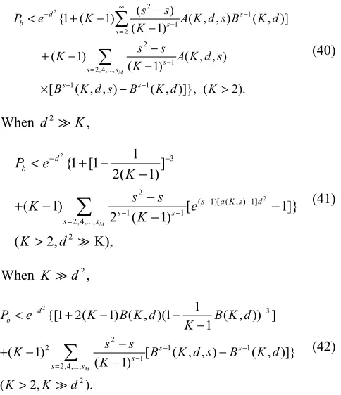
Fig 13. Simulation comparisons of (η, d2) relations for

different h t( ) [12] ( 5

1 10 b

P = × − , equivalent noise bandwidth

It can be seen that whenη≥6, Relation threshold 2

0 / b

d ≜E N (at BERP_b= ×1 10 linear relation, which is identical to the conjecture

Conclusion: The performance of OVTDM than the M-QAM, Especially when spectral Performance of OVTDM begin to go beyond The lager the η, the higher the gain over Shannon

6. OVTDM with Pre-Coding

In a pre-coded OVTDM system, the binary Fig.14 is not directly from the source but output. Fig.14 are some simulations employing and TPC (64, 57) respectively. TPC is the Turbo Product Code or Turbo Array Code. column codes of them are BCH (64, 57)

Novel High Spectral Efficiency Waveform Coding-OVTDM

Bit error probability performances of OVTDM with different

for OVTDM employing bandwidth)

between η and the 5

1 10− ) is roughly a conjecture of [12]. OVTDM is much better spectral efficiencyη≥6, beyond Shannon limit.

Shannon limit.

binary (+1,-1) input of from a pre-coded employing TPC (64, 51) the abbreviation of Code. The row and and BCH (64, 51)

respectively. The code rate respectively and (51/64)2=0.6350.

Fig 14. The spectral efficiency of TPC bandwidth, h2(t) [12], Pb 1 105

−

= × )

It can be seen that the pre-coding spectral efficiency of OVTDM spectral efficiency of OVTDM gain will become lower. For other that the same conclusion will be

7. OVTDM in Random

Channel

A OVTDM performance Channel

The performance of OVTDM time dispersion) channel is studied receiver, Optimum detection is MLSD. As comparison a high order efficiency η with different employed. Because of that OVTDM implicit diversity gain, that “multipath diversity”, the larger diversity gain of the OVTDM

extra diversity for the system employing the high order QAM can’t be

fading channel.

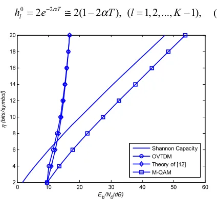
Fig.15 shows the bit error OVTDM with parameter (K1=1, raised cosine multiplexing waveform fading channel. As comparison explicit multiple diversity are error probability curve of such with the 7th order explicit diversity 4dB gain (at BER 5

1 10

b

P = × − ). OVTDM

respectively are (57/64)2=0.7932 ，

TPC pre-coded OVTDM (equivalent noise

coding gain is larger when the OVTDM is low. However when the OVTDM is getting higher pre-coding other kind pre-coding we believe

be obtained.