Published online June 30, 2013 (http://www.sciencepublishinggroup.com/j/acis) doi: 10.11648/j.acis.20130103.12
Development of a model for simultaneous cost-risk
reduction in JIT systems using multi-external and local
backup suppliers
Faraj El Dabee, Romeo Marian, Yousef Amer
School of Engineering, University of South Australia, South Australia, Australia
Email address:
[email protected](F. E. Dabee), [email protected](R. Marian), [email protected](Y. Amer)
To cite this article:
Faraj El Dabee, Romeo Marian, Yousef Amer. Development of a Model for Simultaneous Cost-Risks Reduction in JIT Systems Using Multi-External and Local Backup Suppliers. Automation, Control and Intelligent Systems. Vol. 1, No. 3, 2013, pp. 42-52.
doi: 10.11648/j.acis.20130103.12
Abstract:
In many organisations, Just-In-Time (JIT) implementation plays a significant role in minimizing their excessive costs, and increasing their efficiency. However, the risks accompanying JIT strategies are often overlooked and affect system processes disrupting the entire chain of supply. This paper proposes an inventory model that can simultaneously reduce costs and risks in JIT systems. This model is developed in order to ascertain an optimal ordering strategy for procuring raw materials by using multi-external suppliers and local backup supplier to reduce the total cost of the products, and at the same time to reduce the risks associated with JIT supply within production systems. The effectiveness of the developed model is tested using an example problem with inbuilt disruption. A comparison between the cost of using the JIT system and using the inventory system shows the superiority of the use of the inventory policy.Keywords:
Lean Manufacturing, Just-In-Time (JIT), Production System, Cost-Risk Reduction, Inventory Model, External Supplier, Local Backup Supplier1. Introduction
In today’s competitive global markets, customers seek to obtain their supplies whilst simultaneously obtaining the cheapest prices irrespective of where they are produced. This leads organisations to implement new techniques, in order to reduce the costs of their products and to insure their position in the marketplace [1]. Lean manufacturing is a philosophy, which may be used to assist production systems to reduce their waste, and to increase the activities that add value to the end product to increase its attraction within its market segment [2]. This approach is conceptually simple which has earned it wide popularity. By understanding these foundational concepts and principles, lean manufacturing may be more easily applied [3].
The main task of the lean manufacturing system is to locate the major sources of waste which are then to be eliminated by the application of a large number of tools such as JIT and production smoothing [2]. JIT is considered as one of the significant lean manufacturing tools that can be used within organisations leading to improvement on a
continuous basis including the flow of materials and information, management of human resources, improved throughputs, costs reduction, and elimination of wastes and non-value added activities [4].
Most international organisations have implemented lean manufacturing tools such as Just-in-Time (JIT) in their processes to reduce their costs and to improve their efficiencies [1]. However, they tend to ignore the risks arising from these goals. These risks will impact on their processes disrupting the entire supply chain.
The rest of this paper is organised as follows: Section 2 reviews some of the literature on JIT, and cost and risk modelling. The problem illustrating JIT implementation is described in section 3. Section 4 presents the proposed model formulation to reduce costs and their risks in JIT systems. In section 5, a simplified problem is provided to illustrate the application of the developed model. Section 6 discusses the findings from implementing the developed model in a simplified problem. Finally, section 7 summarises and concludes this paper.
2. Literature Review
Just-in-Time (JIT) is a Lean manufacturing tool that can be utilised to improve organisations’ efficiency. It is a manufacturing pull system, which can be used for planning and controlling operations, in order to produce, and supply the required products at the correct place, when they are required, and at the right ordered amounts [6], [7]. The main principles of JIT include: high quality, small lot sizes, and regular deliveries in short lead times, close contact with suppliers [8]. The appropriate use of JIT in manufacturing can reduce waste and increase productivity, efficiency, profit, and customer satisfaction [9], [10]. According to Tourki [10], some critical principles such as people involvement, training and education, supplier relations, waste elimination, Kanban or pull system, uninterrupted work flow, and total quality control are used for successful implementation of JIT system. In addition, JIT is highly beneficial for many companies, as the literature indicates that the efficiency gained from the implementation of JIT in production processes translates in accelerated productivity. Inventory levels for manufacturing dropped from 50 days to 40 days during 1999 and 2000 in United States. This indicates the importance of JIT implementation for manufacturing production by achieving operational efficiency [11]. Furthermore, it is a critical tool that can also be utilized for the purpose of managing the external activities associated with an organisation including that of purchasing, as well as distribution. Three elements included in case of JIT are: JIT production, JIT distribution and JIT purchasing [2].
Recently, researchers have searched for an economic quantity model for production systems following a JIT approach for ordering raw materials and the shipping processes. Different models can be utilised for the purpose of ensuring reduction in the level of cost and risk in case of JIT systems. For instance, one such model type that can be utilised for achieving cost efficiency is the lot size reduction model. This model emphasizes that by ensuring reduction in the lot size, it can become possible to achieve a reduction with respect to the level of the cost required in performing the delivery of finished products to final consumers [12]. Fahimnia et al. [13] developed a mixed integer formulation for optimising a two-echelon supply network. They concluded that by implementing the
developed model in a case study, it is clear that by considering all production costs prove the effectiveness of this model in the real applications. A higher lot size unnecessarily increases cost and some components of risk, while reducing others. As a result, the lot size risk reduction model can be utilised in order to ensure an optimum lot size and thereby, efficient management of risk from the lot size can ultimately become possible to achieve cost efficiencies. An operation model may also be used for the purpose of JIT scheduling which explains each and every process included in the JIT system. Thus, by way of identifying the stages of JIT systems, necessary actions can be taken for the purpose of achieving cost efficiency in the operation [14].
Sarker and Khan [15] developed a general cost model for the two-stage batch environment taking into consideration a limited rate of production. This model can be utilised to ascertain the product batch-sizes and order-sizes of raw materials, so reducing the total cost that meet the same batches of products, at fixed intervals, to the buyers. Yang and Pan [12] investigate a JIT purchasing model where a single vendor supplies a single purchaser with a product. Their work presents an integrated inventory model, which minimizes the sum of the ordering cost, holding cost, quality improvement and crashing cost by optimizing the order quantity, lead time, process quality and the number of deliveries to provide a lower total cost, higher quality, smaller lot size and shorter lead time. Therefore, applying JIT methods such as small lot size, lead time reduction and quality improvement play a significant role in achieving JIT purchasing goals. In their article, a stochastic model, which includes two stages, was developed by Carneiro et al. [16] to optimise investment portfolios within an oil supply chain in Brazil. Three sources of uncertainty are considered by adopting the conditional value-at-risk (CVaR) as a risk measure within six oil refineries, in order to minimise the expected net present value (ENPV) in the supply chain. Additionally, Julka et al. [17] propose a unified, flexible, and scalable framework for modelling, monitoring and management of refinery supply chains. This framework has two basic elements: object modelling of supply chain flows and agent modelling of supply chain entities. Three classes of agents, emulation, query, and project agents are used for methodologies required for decision-support systems. It is essential to define the optimum production lot size and the order quantities of associated raw materials simultaneously. This could be done by treating the production and purchasing as modules of a single system, minimizing the total cost of the system [15].
supplier reliability, and supplier failure correlation and their impacts on the organization’s preference. He also mentions that common dual sourcing can protect organisation from any disruption impacts due to receiving deliveries from both in case of one supplier is disrupted. Simchi-Levi et al. [19] point out the risks associated with a JIT system in cases of unforeseen disasters disrupting supply chain such as what eventuated with some auto manufacturers following Sept. 11, 2001. They emphasise that sharing risks throughout supply chain parties has a significant impact on them.
Dimakos and Aas [20] presented a new method to model the required total economic capital required, in order to strengthen a financial organization against possible losses. The system was implemented in the Norwegian financial group DnB’s system for risk management. It is concluded that the total economic capital was reduced by 20% of the actual rate for a one year. Also, Gaivoronski et al. [21] presented an approach for considering a cost–risk balanced process to manage the scarce water resources in conditions of uncertainty. A new technique was modelled relating to a re-optimization phase that allows users to organise emergency strategies by adopting the barycentric value as a new target, which resulted in drastic risk reduction in resource delivery. In addition, Jose [22] clarifies how risk management sources in a project´s innovation can be better managed through a modelling process. Although the innovation management relevance is uncertain, several methods of risk management have been proposed. This article focuses on the formation and management of uncertainties in a context and the deployment of risk management techniques. By using a general model of innovation to manage the parameters of risk creation, the risk management process is applied to a specific case. El Dabee et al. [23] developed a mathematical model to reduce the total cost of the products, and at the same time to reduce the risks arising from this cost reduction within production systems by using external suppliers for supplying raw materials to the production systems. They concluded that comparing the use of a JIT system with the use of a specific amount of inventory during a limited period of time had a significant impact on the production system.
According to the literature review related to JIT, all developed models were used to reduce either cost or risk independently. It is clear that risks have an adverse impact in organisations’ performance, which causes an increase in their total costs and at the same time reduces their efficiency. Therefore, risks should be assessed by identifying, evaluating, and measuring them, in order to reduce the undesired effects they cause within these organisations.
3. Problem Description
In this paper, it is assumed that a distribution network consists of multiple external suppliers. This is due to
pricing variances for the same product in different markets. The materials are transported from different manufacturers to the production system, which in turn produces the final product for sale to wholesale or retail outlets. Also, the raw materials are replenished instantaneously to the production system to meet JIT requirements. To avoid any risks that arise from possible disruptions occurring to the external supply chain, it is assumed that the production system is capable of obtaining the raw materials required for full production up to the finished product from local backup suppliers at a higher cost but in a shorter lead time.
4. Model Development
All notations and assumptions, decision variables, parameters, and mathematical formulations will be described as follows:
4.1. Assumptions
The model formulation is based on the following assumptions:
The ordering cost of raw materials is a at fixed rate for each order regardless of the order size;
The utilities cost of the final product is a percentage of total cost of the product that can be changed by the inventory batch size;
The final product price is at a fixed rate regardless of the inventory batch size;
The raw materials are supplied by the regular external supplier if there is no disruption occurs; The raw materials can be purchased from the local backup supplier when one or more of the regular external suppliers are disrupted;
The cost of raw materials from the local backup supplier SLB can be considered as a percentage of their cost when they are purchased from the regular external suppliers depending on its reliability (RS); The worker cost required for producing the final product per time unit is a fixed rate per time unit; The risk cost arising from the likelihood of risk occurrence is a percentage rate depending on its impact on the production system;
The duties cost is incurred if raw materials can be supplied by an external supplier; and
The transfer price required to procure raw material from the regular external supplier can be considered as a percentage of its total cost CM.
4.2. Notations
The following notations are used in the proposed model:
CT: Total cost required to produce one product in
monetary unit (MU);
CM: Raw material cost required for producing one
product (MU);
CO: Ordering cost of raw materials (MU);
system warehouses (MU);
CUM: Unit cost of the raw material at the beginning of
that cycle (MU);
CR: Risk cost arising from disruption occurrence (MU);
CLi: Labor cost rate per labor time in operation i
(MU/hr);
Ctr: Transportation cost for delivering raw materials to
the production system (MU);
CP: The purchasing cost of the raw materials that are
required to produce the product (MU);
CU: Utilities cost of the final product (MU);
CD: Duties cost arising from procuring raw material from
an external supplier (MU);
CUH: The cost that is carried per unit during each cycle
(MU);
TPi: Transfer price required for procuring raw material i
from an external supplier i (MU);
Di: Duty rate (%) per price of raw material i supplied by
an external supplier (MU);
tp: The percentage rate of raw material cost (MU);
TS, n, m: Tensor for transportation cost per critical
measurement (MU);
S: Origin of ordered raw materials;
V: Destination of required raw materials;
mi: Transportation mode for transporting raw material i
to its customer;
tm: Critical transportation measurement of raw materials shipped using transportation mode m;
SEi: Raw material external supplier i;
SLBi: Raw material local backup supplier i;
IF: Indicator function for duty with a value 1 or 0. 1 if the supplier and the production facility are in the same country and 0 otherwise;
Mi: raw material types required in producing one unit of
product i;
LH: Likelihood of occurrence for risk in the supply chain;
I: Impact of risk occurrence in the supply chain; and
%TRS: Total risk score percentage value.
4.3. Parameters
dP: Customer demand for the final product in a period
(unit);
NO: Number of operations required for producing one
product (unit);
NW: Number of workers required to produce one product
(unit);
Nh: Number of working hours for producing the final
product (unit);
NP: Number of parts required to produce one product
(unit);
NS: Number of external suppliers required to supply raw
materials to the production system (unit);
CW: Worker cost required for producing the final product
per time unit (MU);
RS: The reliability of supplier reflects the availability for
supplying raw materials at the planned time (0- 1);
hi: Operation time required to produce a product i (hr);
and
Pi: Final price per unit of final product i sold to the
customer (MU).
4.4. Decision Variables
QM: The quantity of raw materials ordered in each patch
(unit); and
LT: Lead-time in time unit taken between placing and receiving the placed order (day).
4.5. Model Formulation
A general cost model is developed considering supplier of raw material point of view. This model is utilised to ascertain an optimal ordering strategy for obtaining raw materials batch size using both external and local backup suppliers to minimize the total cost of the final products and its risk effect in JIT systems. It is built to determine the total cost of producing the final product within production systems. The total cost of this product can be found by:
T RM W U R
C =C +C +C +C (1)
Also, for the regular external and local backup supplier,
CRM includes the sum of costs CO, CH, CP, Ctr, CDand TP.
Therefore, it can be calculated as:
RM O H P tr D
C =C +C +C +C +C +TP (2)
Where, CO as the cost of ordering and receiving an
amount of raw materials each order that can be calculated as: 1 P i N O O i C C =
=
∑
(3)Also, the rate of CH equals:
1 P i N H UH i C C =
=
∑
(4)CP is the unit cost of the raw material at the beginning of
that cycle CUR that equals:
1 P i N p UM i C C =
=
∑
(5)Ctr as a component of CM can be calculated as:
, , 1 S V m i N tr m S i
C t T
=
= ×
∑
(6)CD is the duty cost arises from supplying raw materials
by a regular external supplier SEj to the production system.
It means that for local backup supplier SLB, there are no
production system. It can be calculated as: 1 1 (1 ) S P i N N
D M j j
i i
C C IF D
= =
=
∑ ∑
− × (7)TP as a transfer price for procuring raw material from a regular external supplier SEi can be calculated as:
1 1 S P i N N j M i i
TP tp C
= =
=
∑ ∑
× (8)Therefore, CRMcan be calculated as follows:
, ,
1 1 1 1
1 1 1 1
(1 )
p P P S
i i i j
S S
P P
i j i
N N N N
RM O UH UM m S V ml
i i i j
N N
N N
M j j P M
i j j i
C C C C t T
C IF D t C
= = = = = = = = = + + + × + − × + ×
∑
∑
∑
∑
∑ ∑
∑∑
(9)However, CP, as the unit cost of raw material i (CUMi)
procured from local backup supplier SLBj at the beginning
of that cycle can be calculated as:
1
P
i N
p UM SLB
i
C C R
=
=
∑
× (10)Also, the worker cost CW can be found as:
1 1
O O
i i
N N
W W L i
i i
C C C h
= =
=
∑
=∑
× (11)In addition, CU is the utilities cost that can be considered
as a raw material cost percentage of the final product. It equals: 1 % P i N U RM i C C =
=
∑
(12)Cpt is the cost of the part of raw material that equals
Pt O H P tr D W U
C =C +C +C +C +C +TP C+ +C (13)
Furthermore, CR as a risk cost can be calculated by the
following equation: 1 1 % ( / ( )) P i P i N
R i M
i
N
M i
C TRS C
LH I Max LH I C = = = × = × × ×
∑
∑
(14) Finally,T Pt R
C =C +C (15)
CT can be calculated in case of using the regular external
supplier for procuring raw materials as follows:
, ,
1 1 1 1
1 1 1 1
1 1 1
(1 ) (1 )
% ( / ( ))
p P P S
i i i j
S S
P P
i j i
O P P
i i i
N N N N
T O UH UM m S V ml
i i i j
N N
N N
M j j P M i j j i
N N N
L i M M
i i i
C C C C t T
C IF D t C
C h C LH I Max LH I C
= = = = = = = = = = = = + + + × + − × + + × + × + + × × ×
∑
∑
∑
∑
∑∑
∑∑
∑
∑
∑
(16)Also, when raw materials are supplied by the local backup supplier, CT can be found as:
, ,
1 1 1 1 1
1 1
% ( / ( ))
p P P S O
i i i j i
P P
i i
N N N N N
T O UH UM m S V m L i
i i i j i
N N
M M
i i
C C C C t T C h
C LH I Max LH I C
= = = = = = = = + + + × + × + + × × ×
∑
∑
∑
∑
∑
∑
∑
(17)According to [23], the proposed model was tested in the simple process for assembling a brushless DC electric motor (BLDC). It was used to ascertain the decision variables effect on other studied parameters within the production system.
5. Example Problem
The mathematical model proposed in section 4 has been tested with a simple assembly process for a landline phone. It uses multiple, identical operations to assemble five individual parts Mi into the finished product (NP= 5) namely,
transmitter, receiver, push-button, ringer or audible indicator, and a small assembly of electrical parts (circuit-board). It is assumed that a production system purchases raw materials in a fixed size from three different regular external suppliers (NS= 3). These raw materials are
delivered at a fixed interval of time when they are needed (JIT system). Parts 1 and 2 are supplied by the supplier SE1,
which need three weeks (LT) to arrive, parts 3 and 4 are supplied by the supplier SE2, which require five weeks to
arrive, and Part 5 is supplied by the supplier SE3, which take
four weeks to arrive. The production system includes four operations conducted by four workers (W1, W2, W3, and W4
respectively). The number of working hours Nh is 8 hours a
day during 5 days per week, each worker has a fixed wage
CWi valued 12 monetary unit (MU)/ hour. Operation 1
assembles parts 1 and 2 and transfers them to operation 2, which assembles parts 3 and 4, and then transfers them to operation 3. Operation 3 assembles parts 5, and finally transfers the product to operation 4, which tests and places the final product in packaging before sending it to the sales department. The production facility produces 70 units per day, and it purchases raw materials from the three different regular external suppliers SE1, SE2, and SE3 (if no disruption
occurs) and two local backup suppliers SLB1 and SLB2 (in the
conditions. It is assumed that the utilities cost CU is equal to
10% of the raw material cost of the final product. It is also assumed that Parts 1, 2, 3, and 4 can be supplied to the production system by SLB1 with a rate of 150% of their cost
when they are purchased from the regular suppliers SE1 and
SE2 and Part 5 can be procured from SLB2 with a rate of 160%
of its cost if they are purchased from the regular suppliers
SE3. Finally, the end customer purchases the final product
by 82 MU. Figure 1 shows the supply chain for this production system.
Figure 1. The supply chain for the production system
However, many risks result from delays in the delivery-time of these materials to the production system. These may arise from risks caused by physical, social, legal, operational, economic and political factors. These factors can affect and disrupt the production system and all the supply chain parties. Therefore, this paper studies the
effects of these factors on the case study of a production facility.
The next step is to identify supply chain risks facing the production facility. Table 1 includes the main supply chain risks potentially facing the production/ marketing of landline phones and their impact within the production system. Risk identification was prepared based on what is perceived as the effect of a disruption or change in demand on the production facility. It may also be approached by investigating all possible root causes of supply chain issues. According to [24], risk can be assessed by two common approaches; the likelihood of the occurrence of an (undesirable) event, and the negative ramifications of the event. Therefore, the total risk score can be calculated by multiplying those scores together.
The risks H1, H2, and H3 may result from increasing the
lead time of raw materials of external suppliers SE1, SE2, and
SE3 respectively to arrive at the manufacturing plant at the
planned time. The likelihood of the occurrence of such risks might arise as a result of some factors such as natural and man-made disasters, and economic crises (currency evaluation/ strikes). All of these mentioned risks will disrupt the production system, and at the same time will affect the other parties in the supply chain. However, impacts of these factors can be avoided by keeping a sufficient inventory within the production facility. An inventory is an important supply chain driver because changing inventory policies can dramatically improve the supply chain's efficiency and responsiveness that makes it able to maintain its permanent production during the disruption time.
Table 1. Risk assessment of the landline phone in production system
Risk
Symbol Risk Product Effect
Likelihood (1 - 5)
Impact
(1 - 5) % Total Risk Score
H1 External supplier 1 cannot supply raw materials on
the scheduled time. All product 2 2 4/25= 16%
H2 External supplier 2 cannot supply raw materials on
the scheduled time. All product 2 4 8/25= 32%
H3 External supplier 3 cannot supply raw materials on
the scheduled time. All product 2 3 6/25= 24%
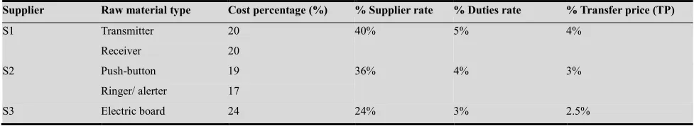
The main cost drivers in a landline phone are: transmitter, receiver, push-button, ringer or signaler, and populated circuit board. They are shown in Table 2 as a percentage
rate of the total cost of the phone. This table also illustrates the cost percentage rate, incurred duties, and transfer price for each supplier.
Table 2. Cost drivers in Landline phone
Supplier Raw material type Cost percentage (%) % Supplier rate % Duties rate % Transfer price (TP)
S1 Transmitter 20 40% 5% 4%
Receiver 20
S2 Push-button 19 36% 4% 3%
Ringer/ alerter 17
6. Results and Discussion
In this section, the proposed model will be used to ascertain the effect of decision variables on other parameters examined within the production system. The findings of this paper are organised in three cases as follows:
6.1. Case I
The impact of lead time on cost types of the final product will be investigated for a scenario of having disruption from an external supplier. This prompts sufficient stock keeping from the external supplier to prevent any likelihood of stock running out.
The findings illustrated in Figure 2 show that if the supplier 1 has disruption for any reason, keeping different amount of raw materials in warehouses (1-35 days) have direct impact on the total cost arising from the risk cost associated with the supplier. Keeping raw materials in the warehouses have high impact on the earned profit. From this figure, it is clear that the production system is able to procure sufficient raw materials to produce the final product for 29 days with an appropriate profit. That is because the external suppliers offer sales discount to their customers for purchasing any extra amount of raw materials. Therefore, it is clear that the net profit increases in the beginning of each week and then gradually decreases until the week ends.
Figure 2. Lead time and its impact on net profit and risk cost arising from external supplier 1 disruption
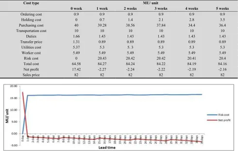
Table 3 demonstrates the results of some cost types calculated using the developed model equations. The maximum duration used for keeping a limited amount of raw materials is 5 weeks based on lead time for external suppliers. It shows that if any disruption affects supplier 2
who supplies some an amount of raw material types used for production, then keeping safety stock of these raw materials in warehouses (1-5 weeks) at different periods of lead time have a direct impact on risk cost.
Figure 3. Lead time and its impact on net profit and risk cost arising from supplier 2 disruption
Table 3 shows increase in the utilities and risk costs, whereas the purchasing cost decreases. However, the
stock amount for 1-35 days give a negative profit rate. From Figure 4, it is also clear that there is a striking impact on the risk cost, when supplier 3 is disrupted. This is
because of the impact of the supplier risk cost arising from this disruption.
Table 3. Effects of lead time on cost types arising from disrupting external supplier 2
Cost type MU/ unit
0 week 1 week 2 weeks 3 weeks 4 weeks 5 weeks
Ordering cost 0.9 0.9 0.9 0.9 0.9 0.9
Holding cost 0 0.7 1.4 2.1 2.8 3.5
Purchasing cost 40 39.28 38.56 37.84 34.4 36.4
Transportation cost 10 10 10 10 10 10
Duties 1.66 1.43 1.43 1.43 1.43 1.43
Transfer price 1.31 0.89 0.89 0.89 0.89 0.89
Utilities cost 5.37 5.3 5. 3 5.3 5.3 5.3
Worker cost 5.49 5.49 5.49 5.49 5.49 5.49
Risk cost 0 20.43 20.42 20.42 20.41 20.4
Total cost 64.58 84.27 84.24 84.22 84.19 84.16
Net profit 17.42 -2.27 -2.24 -2.22 -2.19 -2.16
Sales price 82 82 82 82 82 82
Figure 4. Lead time and its impact on net profit and risk cost arising from supplier 3 disruption
6.2. Case II
Keeping the same base case in-point as the first, the impact of lead time on cost types of final product will be investigated where stock is procured from local backup supplier. This case assumes that the external supplier is not able to meet supplier demand due to the disruption.
By using local backup suppliers for supplying the required raw material in the event of any disruption
occurring from the three external suppliers, stoppage of production caused by a lack of raw materials can be easily avoided. However, this will increase the purchasing and risk cost that depends on the reliability of these suppliers. Figure 5 shows the effects of lead time on the net profit and the risk cost arising from the disruption caused by external supplier 1. This prompts the use of local backup supplier 1 to supply the required amounts of raw materials in different periods of lead time.
Figure 6 also illustrates the lead-time impact on the net profit and the risk cost arising from the disruption caused by external supplier 2. This prompts the use of local backup
supplier 1 to supply the required amounts of raw materials in different periods of lead time.
Figure 6. Lead time and its impact on cost types arising from external supplier 2 disruption using local backup supplier 1
In Figure 7, it is clear that the lead time has marked impact on the total cost arising from the disruption occurring from supplier 3 if the local backup supplier 2 is
used to supply the required amount of raw materials in different periods.
Figure 7. Lead time and its impact on cost types arising from supplier 3 disruption using local backup supplier
6.3. Case III
In this case, the two cases are compared to find the optimum quantity of required raw materials that give an appropriate profit during the disruption period.
Figure 8 illustrates the comparison between the net profit and risk cost arising from producing final product if disruptions occur from external supplier 1. This compares the case of solely relying on an external supplier 1 or using
local backup supplier 1. It can be observed that if supplier 1 has disruption, the cost arising from keeping inventory during this time using local supplier is less than the cost using the same supplier. Therefore, it can be observed that working with a 3 weeks inventory from a local backup supplier during the disrupted time gives a reasonable profit for the production system.
Figure 9 illustrates a similar comparison for the case of supplier 2 and a local backup supplier. It is clear that if supplier 2 is disrupted, the cost arising from keeping
inventory during this time using local supplier is also less than the cost using the same supplier.
Figure 9. Comparison between the net profit and risk cost arising from supplier 2 disruption using the disrupted supplier and local backup supplier 1
The same result has been found in case of supplier 3 is disrupted from supplying raw materials to the production system. Figure 10 shows that by comparing the total cost arising from keeping safety stock amount within the
production facility using the regular external supplier 3 and local backup supplier 2, the risk cost arising from keeping inventory during this time using local supplier 2 is also less than the risk cost using the same supplier.
Figure 10. Comparison between the net profit and risk cost arising from supplier 3 disruption using the disrupted supplier and local backup supplier 2
7. Conclusion and Further Research
This paper presented a mathematical model for a simultaneous cost-risk reduction in JIT systems. It was developed to determine an optimal strategy for supplying raw materials to the production systems by using regular multi-external and local backup suppliers in case of the occurrence of likely disruption such as natural and man-made disasters, and economic crises. By implementing the model in a simplified example, it is concluded that comparing the use of a JIT system with the use of a specific amount of inventory during a limited duration had a significant impact on the production facility especially, by using the local backup supplier during the disruption time. This means that by using strictly JIT, the production system
will be stopped completely during supply disruption. However, by keeping a sufficient inventory, the production system can produce its final products but with a limited profit. Thereby JIT principles can be effectively applied for satisfying customer requirements at a minimum inventory cost with a minimum level of risk.
References
[1] C. Canel and B. M. Khumawala, “International facilities location: a heuristic procedure for the dynamic uncapacitated problem,” International Journal of Production Research, vol. 39, pp. 3975-4000, 2001.
[2] F. Abdullah, “Lean Manufacturing Tools and Techniques in the Process Industry with a Focus on Steel,” PhD thesis, University of Pittsburgh, 2003.
[3] A. Badurdeen, “What is Lean Manufacturing?,” 2006, [Online],
http://www.learnleanblog.com/2006/12/what-is-lean-manufa cturing.html [Accessed 07.11.2011].
[4] B. Fahimnia, R. Marian and B Motevallian, “Analysing the hindrances to the reduction of manufacturing lead-time and their associated environmental pollution, International Journal of Environmental Technology and Management (IJETM), ISSN 1466-2132, vol. 10, no. 1, pp. 16-25, 2009.
[5] Y. Monden, Japanese Cost Management. World Scientific, 2000.
[6] T. C. E. Cheng and S. Podolsky, “Just-in-time manufacturing: an introduction,” New York, Chapman & Hall, 1996.
[7] R. A. Hokoma, M. K. Khan and K. Hussain, “The Present Status of Quality and Manufacturing Management Techniques and Philosophies within the Libyan Iron and Steel Industry,” TQM Journal, vol. 22, no. 2, pp. 209-221, 2010.
[8] Z. X. Chen and B. R. Sarker, “Multi-vendor integrated procurement-production system under shared transportation and just-in-time delivery system,” The Journal of the Operational Research Society, vol. 61, pp. 1654-1666, 2010.
[9] Y. Li, K. F. Man, K. S. Tang, S. Kwong and W. H. Ip, “Genetic algorithm to production planning and scheduling problems for manufacturing systems,” Production Planning & Control, vol. 11, no. 5, pp. 443-458 , 2000.
[10] T. Tourki, “Implementation of Lean within the Cement Industry,” PhD thesis, De Montfort University, 2010.
[11] L. Eldenburg, “Cost Management: Measuring Monitoring and Motivating Performance,” John Wiley & Sons, 2007.
[12] J. S. Yang and J. C. H. Pan, “Just-in-Time Purchasing: an Integrated Inventory Model Involving Deterministic Variable Lead Time and Quality Improvement Investment,” International Journal of Production Research, vol. 42, no. 5,
pp. 853-863, 2004.
[13] B. Fahimnia, L. Luong and R. Marian, “An integrated model for the optimisation of a two-echelon supply network,” Journal of Achievements in Materials and Manufacturing Engineering, vol. 31, pp. 477-484, 2008.
[14] A. Chae and H. Fromm, Supply Chain Management on Demand. Springer, 2005.
[15] R. A. Sarker and L. R. Khan, “An Optimal Batch Size for a Production System Operating under Periodic Delivery Policy,” Computers & Industrial Engineering, vol. 37, pp. 711-730, 1999.
[16] M. C. Carneiro, G. P. Ribas and S. Hamacher, “Risk Management in the Oil Supply Chain: A CVaR Approach,” Industrial & Engineering Chemistry Research, vol. 49, no. 7, pp. 3286-3294, 2010.
[17] N. Julka, R. Srinivasan and I. Karimi, “Agent-Based Supply Chain Management—1: Framework,” Computers and Chemical Engineering, vol. 26, pp. 1755-1769, 2002.
[18] B. Tomlin, “Disruption-Management Strategies for Short Life-Cycle Products,” NAVAL RESEARCH LOGISTICS, vol. 56, pp. 318-347, 2009.
[19] D. Simchi-Levi, L. Snyder and M. Watson, “Strategies for Uncertain Times. Supply chain Management Review,” 2002, [Online]. http://www.lehigh.edu/~lvs2/Papers/SCMR.pdf [Accessed 06 November 2012].
[20] X. K. Dimakos and K. Aas, “Integrated Risk Modelling,” Statistical Modelling, vol. 4, pp. 265-277, 2004.
[21] A. A. Gaivoronski, G. M. Sechi and P. Zuddas, “Balancing Cost-Risk in Management Optimization of Water Resource Systems under Uncertainty,” Physics and Chemistry of the Earth, vol. 42-44, pp. 98-107, 2012.
[22] G. V.-H. Jose, “Modelling Risk and Innovation Management,” Advances in Competitiveness Research, vol. 19, no. 3&4, pp. 45-57, 2011.
[23] F. El Dabee, R. Marian and Y. Amer, “An Optimisation Model for a Simultaneous Cost-Risk Reduction in Just-in-Time Systems,” in the 11th Global Congress on Manufacturing and Management, GCMM2012, Auckland, New Zealand, 2012, pp. 190-201.