© Penerbit UTHM
DOI: https://doi.org/10.30880/ijie.2018.10.02.017
Mechanically rational forms of curved surface structures
shaped from the uniform strain elements
Koki Tanaka
1, Katsushi Ijima
1, Hiroyuki Obiya
1, Muhammad Nizam bin
Zakaria
21 Department of Civil Engineering and Architecture, Graduate School of Science and Engineering, Saga University, 1, Honjo, Saga, 840-8502, Japan.
2 Department of Structural and Material Engineering, Faculty of Civil & Environmental Engineering, University Tun Hussein Onn Malaysia, 86400 Parit Raja Batu Pahat, Johor Darul Ta’zim, Malaysia.
Received 01 January 2018; accepted 15 April 2018, available online 07 May 2018
1. Introduction
Curved surfaces with isotropic tension possess equal geometric stiffness all over the surface against the out-of-plane deformation. Since membrane structures keep the shapes with the internal tension, the forms that the tension is isotropic and even are ideal for the membrane structures [1].
There are many methods for obtaining the curved surfaces with isotropic tension. For example, a method is to use triangular elements mechanically modeled on a soap film in the geometric nonlinear analysis for computing the equilibrium forms [2], and there is another one called the updated reference strategy based on FEM discretization [3]. Since the forms determined from the methods keep the balance of the isotropic tension, occasionally joining inner pressure, almost all the methods do not use material stiffness affecting the in-plane deformation and the stiffness may be obstacles to the computation. Many methods proposed, however, are inapplicable to the form finding with conditions slightly varying from the conditions shaping isotropic tension forms, because the iterative computations almost diverge under the condition with no solution.
The paper applies the uniform strain element possessing the material stiffness to the form finding. The element is being generally used for the geometric nonlinear analysis of membrane structures. Since the element has strain energy, the stationary principle of total potential energy precedes the variation related to minimal
surface area. The method is to seek iteratively a balanced form consisting of the uniform strain elements that the errors of the strains against the objective strain are less than the allowable one. The computation is surely stable resulting from using the material stiffness and moreover analyzing tensile forms at all times by setting the objective strain positive.
The method cannot yield only isotropic tension forms under the conditions with a minimal surface, but also forms with the strains varying as narrowly as possible under the conditions impossible to shape minimal surface and forms consisting of compressive elements under gravitation.
2. Algorithm for form finding with the
uniform strain element
The algorithm first computes an equilibrium form from the geometric nonlinear analysis by using a triangular shape, assumed at the start, of each element in stress, and next corrects the triangular shape in non-stress by using the objective strain given in advance and the present shape of the element in equilibrium, and then iteratively repeats the two stages until the errors of the strains in all the elements become in an allowable margin against the objective strain.
The theories in the two stages are the followings. Abstract: The paper proposes a method for finding mechanically rational and practical forms of curved surface by using the uniform strain elements. Numerical methods for form finding already published give exact solutions but the application is restricted to the problems with the conditions possible to form a minimal surface. This is because the methods use the mechanical model without material stiffness but with only the geometric stiffness of isotropic tension. When the uniform strain elements composing a structural form have even isotropic strain in all over the form, the form is an isotropic tension form. Since the uniform strain element has the material stiffness, the method can stably yield a form with the strains varying as narrowly as possible in the curved surface under the condition impossible to shape a minimal surface.
2.1
Geometric
nonlinear
analysis
for
computing equilibrium forms
Since the algorithm always sets the objective strain positive, the inner force all over the form is tensile, so that the equilibrium solution is unique and the geometric nonlinear analysis essentially needing iterative computation is always and surely stable. The paper uses the iteration of Newton-Raphson method.
2.1.1 End force equation of the uniform
strain element
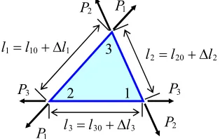
When the nodal positions of the three apexes, as shown in Fig. 1, are given in the coordinates, the positions determine the three lengths of the sides defined as l1, l2 and l3 in Fig. 2. The side lengths of the non-stress element of l10 , l20 and l30 are unvarying until getting an equilibrium form. When the Young’s modulus, Poisson’s ratio and the thickness of the surface are E, ν and t, respectively, the relation between the end forces of the element e, Pe
P1 P2 P3
T
and the elongations
of the sides, le
l1 l2 l3
Tis derived from assuming the strain in the element to be uniform as well as the minute deformation, as follows:
Pekele, (1) where,
ke Et
4(12)A 0
g10 2 l
10 2 g
10g20l10l20 g30g10l30l10 g20
2 l 20
2 g
20g30l20l30
sym. g30
2 l 30 2 , (2)
(1
) / 2, A0: the area of the non-stress element and : the distance between the apex i and the orthocenter in the non-stress element.The stiffness equation of equation (2) indicates that the equation depends on only the side lengths of the non-stress element except the material constants. Therefore, when all the elements have appropriate side lengths in non-stress, the form can be the state in isotropic and even strain.
2.1.2 Equilibrium equation of the uniform
strain element
The nodal forces Ue
U1 U2 U3
T balanced with the end forces of equation (1) at the three nodes connected to the apexes of the element e is,Ue ePe, (3) where,
e
0 2 3
1 0 3
1 2 0
, (4)
and i is the unit vector with the direction of the side i as shown in Fig. 1.
2.1.3 Unbalanced forces and the tangent
stiffness equation for obtaining an
equilibrium form
Since the compatibility between the deformation of the elements and the nodal positions are nonlinear as well as the equilibrium equation (3), obtaining the end forces balanced with the nodal forces U needs the iterative computation. The unbalanced forces Unaturally appear in the computation, as follows:
UU ePe
e
. (5)We define the equilibrium form holding the unbalanced forces less than the allowable force. In order to decrease the unbalanced forces, the tangent stiffness equation gives the displacement from the present nodal positions by using the unbalanced forces and the nodal positions can be renewed.
Differentiating the equilibrium equation gives the tangent stiffness equation, as follows:
U ePe e
ePeePe
KOKG
u, Fig. 1 Nodal position vector and direction cosinevector of the sides in the element.
1 u1 P1 P2 P3 P3 P1 P2 2 3 u2 u3
u, U v, V
w, W
P1
l1l10 l1 l2l20 l2
l3l30 l3 P1
P2 P2
P3
P3 2 1
3
(6) where KO consists of equation (2) of the element stiffness against the in-plane deformation and KOis the tangent geometric stiffness against the out-of-plane deformation. The stiffness matrices in equation (6) are specifically referred to [4].
Applying the unbalanced forces Uto equation (6) gives the displacement
u from the present nodal position.2.1.4 The case of adding axial members
When the strains of the elements composing a form are impossible to be even, adding axial members to the surface structure can sometimes make the strains unify in all the elements.
Several mechanical models of the axial member can be considered in the analysis. However, the axial member without elongation stiffness but with constant axial force will be the most suitable model to the form finding using the uniform strain element. When the axial member has an unchanging axial force N, the end force acts on both nodes i and j connected by the axial member and the tangent stiffness equation of the axial member by the infinitesimal increment of the nodal force at the node i is,
Ui N l (e T)(
ui
uj), (7)where
Ui: the infinitesimal increment of the nodalforce, l: the length of the axial member connecting the two nodes of i and j, e: the unit matrix of 3 by 3, : the unit vector of the direction of the axial member and
ui,
uj: both of the infinitesimal displacements at the two nodes.2.2 Correcting side lengths of the non-stress
element after getting an equilibrium form
The paper shows the two cases of form finding. One is to find a form with even strain all over the form, and the other is to find a form consisting of all the elements in compression under gravitation. In finding the latter form, the main computation is practically to find a suspended form consisting of all the elements in tension under gravitation, and that is, as it were, a computational simulation of the experimental methods that Gaudíy and Otto each individually did [1]. The geometric nonlinear analysis computing an equilibrium form in tension is more stable and more certain than a compressive form.
2.2.1 The case of forms composed by all the
elements with an even strain in tension
Since the strain in the element used in the analysis is isotropic and uniform, the objective strain
0gives the side lengths li0of the non-stress element from the sidelength li of the present deformed element in the equilibrium form, as follows:
li0 li
1
0
. (8)2.2.2 The case of forms composed by all the
elements in compression only under
gravitation
From the present equilibrium form, the side lengths of the element and those of the non-stress element can determine the direction of the principal strain by the angle
pbetween the side 3 and the first principal axis, as shown in Fig. 3.The positions of the apexes in the coordinates of both principal axes are,
, (9)
, (10)
Then, when this case sets the principal strains to the objective strains
10and
20, the positions of the apexes in the non-stress element are,, (11)
, (12)
where the apex 1 is fixed.
The side lengths of the non-stress element are given as the following from the positions of the three apexes in the principal coordinates,
xp l1 l2
l3 (xp2,yp2) (0,0)
p
11 2
3 yp
(xp3,yp3)
. (13)
Correcting the side lengths of the non-stress element by using the objective strain can change the compressive elements to tensile elements in a curved surface suspended under gravitation. After transforming all the compressive elements to tensile ones, turning the curved
surface form upside down in the direction of gravitation gives the form consisting of all the compressive elements.
3. Computational examples
3.1 Rotational hyperboloid and the related
forms
The first example shows that the uniform strain element can shape a rotational hyperboloid that is a theoretical solution of minimal surface. In the form of Fig. 4(a) obtained from using the element, the two of the circular rims are fixed parallel to each other and the normal line of the planes goes through both centers. The rotational hyperboloid can be shaped under the condition that the ratio of the diameter and the distance between the two circles is over 1.51. The ratio of Fig. 4(a) is 2.11, so that the theoretical form exists.
Fig. 4(b) shows the comparison of the two forms, and the computational form well agrees with the analytical form, where r is the distance from the circular center and
h is the distance from the midpoint of the two circles. The computation uses the practical constants of membrane material of Et=88.2kN/m and ν=0.4, and the objective strain is
0 =0.01. The material constant is based on the membrane material of polyester fabric Fig. 4 Computational result of a rotational hyperboloidh
(m)
1.8
0.0
-
1.0
2.0
1.9
1.7
-
0.5
r
(m)
(b) Verification of the computational form.
Theoretical hyperboloid
Computational form
2H=1.89m
2R=4.00m
(a) Computational form.
Fig. 6 Forms related to hyperboloid constants or the objective strain change, the form of Fig.
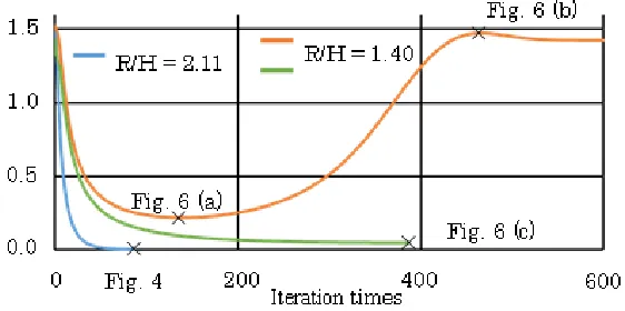
4(a) does not vary at all but the convergent process does. The blue line in Fig. 5 shows the convergent process of the error rate of the strains to the objective strain in the case of R/H=2.11 and that the error rate surely decreases to nearly zero. If the material stiffness is larger than that of this case, the iterative times need more than that. The iterative times mean the times of computing equilibrium forms.
Fig. 5 shows other cases of the ratio R/H also. When the ratio is less than 1.51, any rotational hyperboloid cannot be formed. When the ratio is 1.40, for example, as shown by the orange line in Fig. 5, the maximum of the error rates to the objective strain first decreases but increases after passing the minimum. If we use computational models with no in-plane stiffness, the process will lead to divergence. The method proposed in the paper, however, can give the form that the maximum of the error rates becomes the minimum in the iteration as shown in Fig. 6(a).
Further, proceeding the iterative process in the case of R/H=1.40 changes from Fig. 6(a) to Fig. 6(b). Fig. 6(b) resembles the theoretical minimal surface that is the two disks in the circles of fixed boundaries under the condition of R/H<1.51.
Fig. 6(c) is the form that the three ring frames in compression are attached to the form of Fig. 6(a). The axial forces of the rings are -1.6kN and -0.8kN. The green line in Fig. 5 shows the convergent process in computing the form, and the maximum of error rates decreases to the value of 0.047 less than that in Fig. 6(a).
3.2 A hyperboloid and the form related to
one
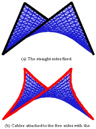
Fig. 7(a) shows a hyperboloid that the fixed circumference in the form consists of the sides of the two
equilateral triangles crossing at right angles. Further, Fig. 7(b) has the four corners fixed that are the same position as Fig. 7(a) and that the cables are attached to the free circumference. The proposed method can yield the forms composed by all the elements with the isotropic strain of nearly
0=0.01 in the two cases, namely both maximums of error rates decrease to the value less than 0.01, as shown in Fig. 8. The material constants used in the computations are the same as that of the previous example.3.3 Compressive curved surface under
gravitation
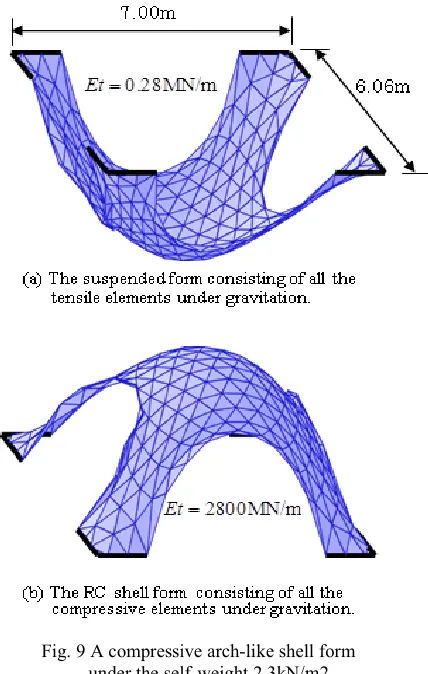
This example shows a mechanically rational form under gravitation. If we take the self-weight of structural material into consideration in form finding, the analysis is impossible to shape a form with isotropic and even strain
all over the curved surface. When structures made of reinforced concrete, however, are the forms with no tensile stress though no even strain, the forms will be
mechanically rational, as Gaudíy and Otto each individually experimented and found the practical forms [1].
The proposed method is just to simulate numerically the experimental procedures. The form of Fig. 9(a) is obtained from the iterative computation correcting side lengths of non-stress elements in order to change compressive strain to tensile strain. The self-weight per unit area is 2.3kN/m2 corresponding to RC plate with 10cm in thickness. Finding the suspended form uses the stiffness of Et=0.28MN/m that is smaller than the real, in order to obtain quickly the form. Then, the form inverted of Fig. 9(b) is obtained from the geometric nonlinear analysis using the practical stiffness of the RC plate of Et=28000MN/m. The side lengths of the non-stress elements are computed from solving equation (1) that the end forces change positive to negative with keeping the absolute value together with inverting the shape. Since the non-stress side lengths are unknown in equation (1), the computation is a nonlinear problem. The change of the material stiffness in equation (1) means that the strains of the elements decrease to 10-4 of the strain of the elements in the suspended form of Fig. 9(a).
4. Conclusion
The paper proposed a method of form finding using the uniform strain elements. The method is to correct side lengths of the non-stress elements according to the objective strain in the equilibrium form obtained from the geometrical nonlinear analysis. The method uses the in-plane stiffness corresponding to real material, though many methods published so far do not need it or regard it as obstacles. The paper shows that using the in-plane stiffness makes the computation robust, so that the method can manage problems of form finding with conditions that does not possess a minimal surface or the method can suggest how to attach cables to make the strains as even as possible in the form.
References
[1] Otto, F. Natürliche Konstruktionen, Stuttgart: Deutsche Verlags-Anstalt GmbH, (1982).
[2] Goto, S., Aramaki, G., Ijima, K., Fukae. Y., Analyses of isotonic curved surface and membrane structure by the method with the separation of the element stiffness, Journal of Structural Engineering JSCE, Vol. 37A, (1991), pp. 307-.
[3] Bletzinger, K.U. Form finding of tensile structures by the updated reference strategy, STRUCTURAL MORPHOOLOGY Towards the New Millennium, Int. Colloq. Nottingham, UK, (1997), pp. 68-.
[4] Ijima, K., Obiya, H., Kido, K. An orthotropic membrane model replaced with line members and the large deformation analysis, International Conference on Textile Composites and Inflatable Structures, Structural Membrane, (2011), CD-ROM.
[5] Ishii, K. Pneumatic Membrane Structure, Design and Application Tokyo: Kogyo Chosakai Publishing Co., Ltd., (1977).
Fig. 8 Convergent process in computing the hyperboloids of Fig. 7