Paper 02-2012-2

_{(UDC: 624.073.2:539.3)}

Functionally Graded Nonhomogeneous Anisotropic Thick Plates. A

Meshless 3D Analysis

Maria S. Nerantzaki

School of Civil Engineering, National Technical University of Athens Email: [email protected]

Abstract

The meshless analog equation method (MAEM) is employed for 3D analysis of thick functionally graded nonhomogeneous anisotropic plates. In this case the response of the plate is governed by three coupled partial differential equations (PDEs) of second order with variable coefficients in terms of displacements, i.e. the counterpart of the Navier equations for the general nonhomogeneous anisotropic body. The system of equations is solved using the new truly meshless method for solving elliptic PDEs developed by Katsikadelis. This method is based on the concept of the analog equation, which converts the original coupled PDEs into three uncoupled Poisson’s equations with fictitious sources, under the original boundary conditions. The fictitious sources, unknown in the first instance, are approximated by multi-quadrics radial basis functions (MQ-RBFs) series. Integration of the substitute equations allows the approximation of the sought solution by new RBFs, which approximate accurately not only the solution but also its derivatives. This permits a strong formulation of the problem. Thus, inserting the approximate solution in the PDEs and in the boundary conditions (BCs) and collocating at a predefined set of mesh-free nodal points yield a system of linear equations, which permit the evaluation of the expansion coefficients of radial basis series, which represent the solution. Numerical results are given which validate the efficiency and the accuracy of the developed solution procedure.

Keywords: Meshless method, thick plates, nonhomogeneous anisotropic elasticity, radial basis functions, analog equation method

1. Introduction

20

the realization of the consistent associated boundary conditions. The Mindlin and Reissner theories have given good approximations as second order theories and several solutions have been developed (e.g. Katsikadelis and Yiotis, 1993). The researcher realized early that all these shortcomings could be overcome if the plate was analyzed a 3-D prismatic body. Three-dimensional structures are governed by the Navier equations of equilibrium and can be analyzed numerically either by domain methods (e.g., finite difference and finite element methods) or by the boundary methods (e.g. boundary element method). However, the above mentioned numerical methods seem not efficient, when the material is nonhomogeneous anisotropic due to the fact that the differential equations that must be solved have variable coefficients. An alternative to these methods could be the so called meshless or mesh-free methods. The radial basis function methods offer an efficient computational tool to solve complicated differential equations (Kansa, 1990) using only nodal points arbitrarily distributed in the domain and on the surface of the body. This method is alleviated from element discretization, as in FEM, or from establishing the fundamental solution, as in BEM. Among them the standard MQ-RBF (multiquadrics radial basis functions) method has been applied to solve several problems. However, this method exhibits certain major disadvantages. The resulting coefficient matrix becomes ill-conditioned as the number of the nodes increases and special techniques are required to circumvent this shortcoming (Kansa and Hon 2005). On the other hand, due to inaccuracy of the derivatives of the approximated solution the strong formulation of the problem may be problematic. More over the accuracy of the solution depends on the shape parameter of the MQs, which, however, can not be specified a priori for an optimum solution. The above drawbacks are overcome by the new meshless RBFs method, the MAEM (Katsikadelis 2006). This method is based on the concept of the analog equation of Katsikadelis, according to which the original equation is converted into a substitute equation, the analog equation, under a fictitious source. The fictitious source is represented by radial basis functions series of multiquadric type. Integration of the analog equation yields the sought solution as series of new radial basis functions. The major advantage of the presented formulation is that it results in coefficient matrices, which are not ill-conditioned and thus they can be always inverted. Moreover, since the accuracy of the solution depends on a shape parameter of the MQs, the position of the nodal points as well as of the two arbitrary integration constants of the analog equation, a procedure is developed to optimize these parameters. This is achieved by minimizing the functional that produces the PDE as an Euler-Lagrange equation (Katsikadelis 2008) under the inequality constraint that the condition number of the coefficient matrix ensures invertibility. This procedure requires the evaluation of a domain integral during the minimization process. This is facilitated by converting the domain integral to a boundary integral using DRM (Katsikadelis 2002). The proposed method is applied here to solve the system of three coupled equations describing the response of an nonhomogeneous anisotropic elastic prismatic body representing the thick plate. Numerical examples are presented, which illustrate the efficiency and accuracy of the method.

21

2. Derivation of the Governing Equations

Consider the 3-D inhomogeneous anisotropic linear elastic body occupying the domain V of the xyz space with boundary S. The equations governing the elastostatic response of the body are

Equilibrium equations: ˆT f 0 (1a)

Constitutive relations C (1b)

Kinematic relations ˆu (1c)

Total potential: 1

2 t

T T

V dV S ds

 _

 _

  _  _ 

 





(1d)

where CCij,( ,i j1,2 , 6) is the constitutive matrix; St is the part of the boundary where

tractions are prescribed. The operator ˆ yields the kinematic relations and is given as

0 0 0

ˆ _{0 0 0}

0 0 0

x y z

y x z

z y x

_{  }    _{  }                  _{  }               (2a) and u v w             _{ }         u , x y z xy yz zx                               _{ }                      , x y z xy yz zx                               _{ }                      , x y z f f f               _{ }           f (2b)

are the vectors of the displacement, stress and strain components and body forces, respectively. Since the body is nonhomogeneous the constitutive matrix is position dependent, that is

( , , )x y z 

C C . This matrix is symmetric, CCT, and nonsingular, det( )C 0.

Introducing Eq. (1b) into (1a) and using (1c) we obtain the equilibrium equations in terms of the displacements

 

 

 

11 12 13 x 0

L u L v L w f  (3a)

 

 

 

21 22 23 y 0

L u L v L w f  (3b)

 

 

 

31 32 33 z 0

L u L v L w f  (3c)

22

2 2 2 2 2 2

11 11 ₂ 44 ₂ 66 ₂ 14 16 46

11 14 16 14 44 46

16 46 66

2 2 2

( , , , ) ( , , , )

( , , , )

x y z x y z

x y z

L C C C C C C

x y x z y z

x y z

C C C C C C

x y

C C C

z                                     (4a)

2 2 2 2 2

12 14 ₂ 24 ₂ 56 ₂ 12 44 15 46

2

26 45 14 44 46 12 24

26 15 45 56

( ) ( )

( ) ( , , , ) ( , ,

, ) ( , , , )

x y z x y

z x y z

L C C C C C C C

x y x z

x y z

C C C C C C C

y z x

C C C C

y z                                        (4b)

2 2 2 2 2

13 16 ₂ 45 ₂ 36 ₂ 15 46 13 66

2

56 34 16 46 66 15 45

56 13 34 36

( ) ( )

( ) ( , , , ) ( , ,

, ) ( , , , )

x y z x y

z x y z

L C C C C C C C

x y x z

x y z

C C C C C C C

y z x

C C C C

y z                                        (4c)

2 2 2 2 2

21 14 ₂ 24 ₂ 56 ₂ 12 44 15 46

2

26 45 14 12 15 44 24 45

46 26 56

( ) ( )

( ) ( , , , ) ( , , , )

( , , , )

x y z x y z

x y z

L C C C C C C C

x y x z

x y z

C C C C C C C C

y z x y

C C C

z                                        (4d)

2 2 2 2 2 2

22 44 ₂ 22 ₂ 55 ₂ 24 45 25

44 24 45 24 22 25

45 25 55

2 2 2

( , , , ) ( , , , )

( , , , )

x y z x y z

x y z

L C C C C C C

x y x z y z

x y z

C C C C C C

x y

C C C

z                                     (42e)

2 2 2 2 2

23 46 ₂ 25 ₂ 35 ₂ 45 26 34 56

2

23 55 46 26 56 45 25 55

34 23 35

( ) ( )

( ) ( , , , ) ( , , , )

( , , , )

x y z x y z

x y z

L C C C C C C C

x y x z

x y z

C C C C C C C C

y z x y

C C C

23

2 2 2 2 2

31 16 ₂ 45 ₂ 36 ₂ 15 46 13 66

2

56 34 16 15 13 46 45 34

66 56 36

( ) ( )

( ) ( , , , ) ( , , , )

( , , , )

x y z x y z

x y z

L C C C C C C C

x y x z

x y z

C C C C C C C C

y z x y

C C C

z                                        (4g)

2 2 2 2 2

32 46 ₂ 25 ₂ 35 ₂ 45 26 34 56

2

23 55 46 45 34 26 25 23

56 55 35

( ) ( )

( ) ( , , , ) ( , , , )

( , , , )

x y z x y z

x y z

L C C C C C C C

x y x z

x y z

C C C C C C C C

y z x y

C C C

z                                        (4h)

2 2 2 2 2 2

33 66 ₂ 55 ₂ 33 ₂ 56 36 35

66 56 36 56 55 35

36 35 33

2 2 2

( , , , ) ( , , , )

( , , , )

x y z x y z

x y z

L C C C C C C

x y x z y z

x y z

C C C C C C

x y

C C C

z                                     (4i)

The boundary conditions on a part of the boundary may be of the following type:

, ,

uu vv ww on Su (5a)

, ,

x x y y z z

t t t t t t on St (5b)

where u v w t t t, , , , ,x y z are prescribed quantities. Mixed type boundary conditions may be also

specified on a part of the boundary, namely combinations of three components, such as two displacement and one traction component or one displacement and two traction components. Attention should be paid if St is the whole surface. In this case, the boundary tractions can not

be prescribed arbitrarily, but they must ensure the overall equilibrium of the body. For this type of boundary conditions, the solution of Eqs (3) is not uniquely determined, because it contains an arbitrary rigid body motion. Therefore, the rigid body motion should be restrained in order to obtain the solution (Katsikadelis 2002). The traction components on the boundary are given as

 

t  n (6)

where n( , , )n n nx y z is the unit vector normal to the boundary. Using (1b) and (1c), Eqs (6) give 11( ) 12( ) 13( )

x

t T u T v T w (7a)

21( ) 22( ) 23( ) y

t T u T v T w (7b)

31( ) 32( ) 33( ) z

24

where the operators Tij are given as

11 11 14 16 14 44 46

16 46 66

( ) , ( ) ,

( ) ,

x y z x x y z y

x y z z

T C n C n C n u C n C n C n u

C n C n C n u

     

   (8a)

12 14 44 46 12 24 26

15 45 56

( ) , ( ) ,

( ) ,

x y z x x y z y

x y z z

T C n C n C n v C n C n C n v

C n C n C n v

     

   (8b)

13 16 46 66 15 45 56

13 34 36

( ) , ( ) ,

( ) ,

x y z x x y z y

x y z z

T C n C n C n w C n C n C n w

C n C n C n w

     

   (8c)

21 14 12 15 44 24 45

46 26 56

( ) , ( ) ,

( ) ,

x y z x x y z y

x y z z

T C n C n C n u C n C n C n u

C n C n C n u

     

   (8d)

22 44 24 45 24 22 25

45 25 55

( ) , ( ) ,

( ) ,

x y z x x y z y

x y z z

T C n C n C n v C n C n C n v

C n C n C n v

     

   (8e)

23 46 26 56 45 25 55

34 23 35

( ) , ( ) ,

( ) ,

x y z x x y z y

x y z z

T C n C n C n w C n C n C n w

C n C n C n w

     

   (8f)

31 16 15 13 46 45 34

66 56 36

( ) , ( ) ,

( ) ,

x y z x x y z y

x y z z

T C n C n C n u C n C n C n u

C n C n C n u

     

   (8g)

32 46 45 34 26 25 23

56 55 35

( ) , ( ) ,

( ) ,

x y z x x y z y

x y z z

T C n C n C n v C n C n C n v

C n C n C n v

     

   (8h)

33 66 56 36 56 55 35

36 35 33

( ) , ( ) ,

( ) ,

x y z x x y z y

x y z z

T C n C n C n w C n C n C n w

C n C n C n w

     

   (8i)

The expression of the total potential, Eq. (1d), is written in terms of displacements as

2 2 2 2 2

11 22 33 44 55

2

66 12 13 23 14

15 16 24 25 26

1 _{{( , , , ( , , ) ( , , )}

2

( , , ) 2 , , 2 , , 2 , , 2 , [ ( , , )

( , , ) ( , , )] 2 , [ ( , , ) ( , , ) ( , , )]

2 ,

x y z y x z y

V

z x x y x z y z x y x

y z x z y y x y z x z

C u C v C w C u v C v w

C u w C u v C u w C v w u C u v

C w v C w u v C u v C w v C w u

w                          



34 35 36 45

46 56

[ ( , , ) ( , , ) ( , , )] 2 ( , , )( , , )

2 ( , , )( , , ) 2 ( , , )( , , )}

( )

x y z

z y x y z x z z y y x

y x z x z y z x

x y z x y z

V S S S

C u v C w v C w u C v w u v

C u v u w C v w u w dV

f u f v f w dV t uds t vds t wds

       

     



_

_

_

_

25

where S S Sx, ,y s are the parts of the boundary on which the tractions t t tx, ,y z are prescribed.

Note that in general it is Sx Sy Sz.

3. The MAEM solution

Let u v w, , be the sought solution. These functions are twice differentiable in V and once on the surface S. Applying the Laplacian operator 2 we obtain the analog equations

2

1( )

u b

  x  2v b2( )x 2w b3( )x (10a,b,c)

where bi bi( ),x i1,2, 3 are unknown fictitious sources. Eqs (10) under the boundary

conditions (5) can give the solution of the problem provided that the fictitious sources ( )

i i

b b x are first established. In this context the fictitious sources are approximated by MQ-RBFs series. Thus, for the displacement u we can write

2 (1)

1 M N

j j j

u  a f 

 



where fj  r2c2 , r x x j , c is the shape parameter and M N, represent the

number of collocation (nodal) points inside V and on S, respectively. Equation (11) is integrated to yield the solution in the form

(1)

1

ˆ

M N j j j

u  a u 



 (12)

where uˆj is the solution of

2_ˆ

j j

u f

  (13)

Eq. (13) is readily integrated as follows.

Since fj f rj( ) depends only on the radial distance r , it will be also uˆj u rˆ ( )j .

Consequently, we can write Eq. (13) in spherical coordinates as





2 2 2

2

ˆ 1

) d du

r r c

dr dr r

 _

 _{  }

 _

 

  (14)

which yields after consecutive integration





4 2 3

ˆ ln

8 24

j

f c f

c r f G

u F

r c r

  _{ }

 _

 _{ }  

  (15)

26

(1)

1

ˆ

M N j j j

u  a u 



 (2)

1

ˆ

M N j j j

v  a u 



 (3)

1

ˆ

M N j j j

w  a u 



 (16a,b,c)

which are forced to satisfy the governing equations and the boundary conditions. For this purpose Eqns (16) are inserted into Eqns (3) and (5) to yield the system of linear equations



Aa b (17)

which permit the evaluation of the 3(M N) coefficients a aj(1), j(2),a(3)j (j1,2, ,M N).

Then the solution is given from Eqs. (16), which can be differentiated and inserted in Eqs (1b) and (1c) to give the strains and stresses at the nodal points. Optimal values of the shape parameter and centers of the multiquadrics as well as of the integration constants G and F can be obtained by minimizing the total potential, Eq. (9), while controlling the condition number of the matrix A to ensure its invertibility. This procedure also minimizes the error of the solution.

4. Numerical Examples

The method is illustrated by the examples below. The thick plate is represented by a three dimensional prismatic body. The interior nodal points are distributed on layers symmetrically placed with respect to the middle surface. The same distribution of the nodal points is employed on the upper and lower surfaces of the plate, while the nodal points on the lateral boundary surface are distributed along line normal to the middle surface. This distribution permits the simulation of the conventional plate boundary conditions. The results have been obtained by programming the previously presented solution procedure in MATLAB language and using its ready-to-use functions for matrix manipulation and minimization. Two square plates, one clamped and one simply supported, have been analyzed.

Example 1. A uniformly loaded clamped square plate

A homogeneous square clamped plate of side a1m and thickness h has been analyzed ( 0 x 1, 0 y 1, 0 z h). The material constants are: E 1.1 10 5kN / m2 and

0.3

  , while the uniform load is _{q1000kN / m}2

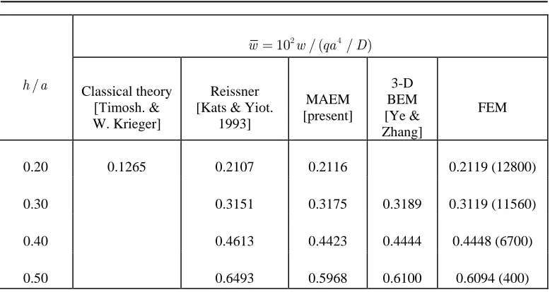
. In Table 1, the computed by the MAEM non-dimensional central deflection w of the plate for different thickness-to-side ratios h a/ ;

3_{/ 12(1} 2₎

27

2 4

10 / ( / )

w w qa D

Classical theory [Timοsh. & W. Krieger]

Reissner [Kats & Yiot.

1993]

MAEM [present]

3-D BEM [Ye & Zhang]

FEM

0.20 0.1265 0.2107 0.2116 0.2119 (12800)

0.30 0.3151 0.3175 0.3189 0.3119 (11560)

0.40 0.4613 0.4423 0.4444 0.4448 (6700)

0.50 0.6493 0.5968 0.6100 0.6094 (400)

Table 1: Central deflection of a uniformly loaded clamped square plate

The FEM solution was obtained using the NASTRA code with solid elements (their number is shown in parenthesis in the Table). Moreover, in Fig. 1 through Fig. 7 the variation of the displacements and stresses along the thickness for the case a1,h0.5 are presented as compared with a FEM solution. The load q1000kN / m2 acts on the surface z 0.

Figure 1. Variation of the transverse displacement w along the thickness at the center of the plate.

/ h a

0 2 4 6 8

x 10-3 0

0.1 0.2 0.3 0.4 0.5

w (m)

z

(m

)

Deflection w at x=0.5 y=0.5

28

Figure 2. Variation of the stress z along the thickness at the center of the

plate.

Figure 3. Variation of the stress x along the thickness at the center of

the plate.

-10000 -800 -600 -400 -200 0 200 0.1

0.2 0.3 0.4 0.5

σ_z (kN/m2)

z

(m

)

σ_z at x=0.5 y=0.5

MAEM FEM

-15000 -1000 -500 0 500 1000

0.1 0.2 0.3 0.4 0.5

σ

x (kN/m 2₎

z

(m

)

σ

x at x=0.5 y=0.5

29

Figure 4. Variation of the displacement u along the thickness at point 0.75, 0.5

x  y of the plate.

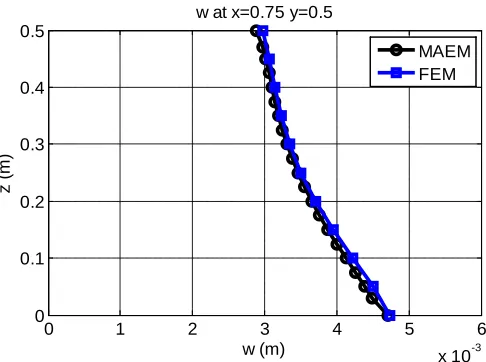
Figure 5. Variation of the transverse displacement w along the thickness at point x 0.75,y 0.5 of the plate.

-1 -0.5 0 0.5 1

x 10-3 0

0.1 0.2 0.3 0.4 0.5

u (m)

z

(m

)

u at x=0.75 y=0.5

MAEM FEM

0 1 2 3 4 5 6

x 10-3 0

0.1 0.2 0.3 0.4 0.5

w (m)

z

(m

)

w at x=0.75 y=0.5

30

Figure 6. . Variation of the stress z along the thickness at point

0.75, 0.5

x  y  of the plate.

Figure 6. . Variation of the stress x along the thickness at point

0.75, 0.5

x  y  of the plate.

Example 2. A functionally graded simply supported square plate

A square simply supported plate made of nonhomogeneous isotropic material is analyzed. The side of the plate is a1 and thickness h0.25. We use a Cartesian coordinate system xyz, with the plane z 0 coincident with the middle surface of the plate. A normal traction

-10000 -800 -600 -400 -200 0

0.1 0.2 0.3 0.4 0.5

σ_z (kN/m2)

z

(m

)

σ_z at x=0.75 y=0.5

MEAM FEM

-600 -400 -200 0 200

0 0.1 0.2 0.3 0.4 0.5

σ_x (kN/m2)

z

(m

)

σ_x at x=0.75 y=0.5

31

(transverse load) qq0sin( )sin( )x y is applied on the upper surface, while the lower surface is traction free. The material is nonhomogeneous and exponentially graded through the thickness, that is EzE e0 k z h( / 1/2), Ex Ey E0; k is a parameter that dictates the material

variation profile through the plate thickness and takes values greater than zero. In the case 0

k  , the plate is fully homogeneous. The numerical results have been obtained with

5 0 1.1 10

E   ,  0.3 and 2

kN / m

0 1000

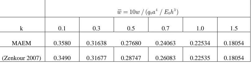
q  using N=238 surface nodal points and M=245 internal nodal points distributed at five layers. Table 2 shows the nondimensional central deflections for various values of the parameter k as compared with those given in Ref. (Zenkour 2007).

4 3

0 0

10 / ( / )

w w q a E h

k 0.1 0.3 0.5 0.7 1.0 1.5

MAEM 0.3580 0.31638 0.27680 0.24063 0.22534 0.18054

(Zenkour 2007) 0.3490 0.31677 0.28747 0.26083 0.22535 0.18054

Table 2: Central deflection of a functionally graded simply supported square plate.

5. Conclusions

In this paper, thick plates made of nonhomogeneous functionally graded and anisotropic material have been modeled as three dimensional prismatic bodies. The analysis has been performed using the MAEM (Meshless Analog Equation Method). The method has been applied successfully to analyze thick clamped and simply supported plates with various thickness-to-side ratios. It incorporates all the advantages of truly meshless methods, while it circumvents the drawbacks due to the use of MQ-RBFs. The efficiency and accuracy of the method is demonstrated by comparing the results with those obtained from other methods developed for thick plate analysis.

References

Kansa, E.J. (1990). Multiquadrics –a scattered data approximation scheme with applications to computational fluid dynamics– II: Solution to parabolic, hyperbolic and elliptic partial differential equations, Computers and Mathematics with Applications, 19, 149-161.

Kansa, E.J. and Hon, Y.C. (2005). Circumventing the ill-conditioning problem with multiquadric radial basis functions: Applications to elliptic partial differential equations,

Computers and Mathematics with Applications, 39, 123-137.

Katsikadelis, J.T. and Yotis, A.J. (1993), A new boundary element solution of thick plates modelled by Reissner’s theory, Engineering Analysis with Boundary Elements, Vol. 12, pp. 65-74.

Katsikadelis, J.T. (2002). Boundary Elements: Theory and Applications, Elsevier Science, London.

32

Katsikadelis, J.T. (2008). A generalized Ritz Method for Partial Differential Equations in Domains of Arbitrary Geometry Using Global Shape Functions. Engineering Analysis with Boundary Elements, 32 (5), pp. 353–367.

Kienzler R. (2002). On consistent plate theories, Archive of Applied Mechanics, 72, 229-247. Timoshenko S. and Woinowsky-Krieger S. (1959). Theory of plates and shells, 2nd ed.,

McGraw-Hill Book Company, New York.

Wang, C.M., Reddy, J.N. and Lee, K.H. (2000). Shear Deformable beams and Plates, Elsevier Science, UK.

Ye, T.Q. and Zhang, D. (1988). Analysis of thick plates by three-dimensional boundary elements, Boundary Elements X, Vol. 3: Stress Analysis (ed. C.A. Brebbia), Springer, Berlin, pp. 425-433.

33

Извод

Функционално распоређене нехомогене анизотропне дебеле плоче.

Безмрежна 3Д анализа

M.S. Nerantzaki

School of Civil Engineering, National Technical University of Athens Email: [email protected]

Резиме

Метода безмрежне аналогне једначине (MAEM) је коришћена за 3Д анализу дебелих функционално нехомогених анизотропних плоча. У овом случају одзив плоче је заснован на три спрегнуте парцијалне диференцијалне једначине (ПДЕ) другог реда са променљивим коефицијентима зависних од померања, тј. ово одговара Навиеовим једначинама за опште нехомогено анизотропно тело. Систем једначина је решен користећи потпуно нову безмрежну методу за решавање елиптичних ПДЕ развијену од стране Кацикаделиса (Katsikadelis). Метода се заснива на концепту аналогне једначине, која преводи оригиналне спрегнуте ПДЕ у неспрегнуте Поасонове једначине са фиктивним изворима, а са оригиналним граничним условима. Фиктивни извори, непознати у почетку, се апроксимирају са мулти-квадратним низовима функција са радијалном базом (MQ-RBFs). Интеграција ових једначина-замена допушта апроксимацију траженог решења новим RBF низовима, који не само да тачно апроксимирају решење већ и његове изводе. Ово допушта јаку формулацију проблема. Према томе, уметање приближног решења у ПДЕ једначине и у граничне услове и колоцирање у унапред дефинисаном скупу од мреже слободних чворова, даје систем линеарних једначина које допуштају одређивање коефицијената развијеног низа са радијалном базом, што представља решење. Дати нумерички резултати потврђују ефикасност и тачност развијеног поступка решавања.

Књучне речи: Безмрежна метода, дебеле плоче, нехомогена анизотропна еластичност, функције са радијалном базом, метода аналогне једначине

References

Kansa, E.J. (1990). Multiquadrics –a scattered data approximation scheme with applications to computational fluid dynamics– II: Solution to parabolic, hyperbolic and elliptic partial differential equations, Computers and Mathematics with Applications, 19, 149-161.

Kansa, E.J. and Hon, Y.C. (2005). Circumventing the ill-conditioning problem with multiquadric radial basis functions: Applications to elliptic partial differential equations, Computers and Mathematics with Applications, 39, 123-137.

34

Katsikadelis, J.T. (2002). Boundary Elements: Theory and Applications, Elsevier Science, London.

Katsikadelis, J.T. (2006). The meshless analog equation method. A new highly accurate truly mesh-free method for solving partial differential equations, Transaction of the Wessex Institute: Modelling and Simulation, Vol. 42, pp. 13-22.

Katsikadelis, J.T. (2008). A generalized Ritz Method for Partial Differential Equations in Domains of Arbitrary Geometry Using Global Shape Functions. Engineering Analysis with Boundary Elements, 32 (5), pp. 353–367.

Kienzler R. (2002). On consistent plate theories, Archive of Applied Mechanics, 72, 229-247. Timoshenko S. and Woinowsky-Krieger S. (1959). Theory of plates and shells, 2nd ed.,

McGraw-Hill Book Company, New York.

Wang, C.M., Reddy, J.N. and Lee, K.H. (2000). Shear Deformable beams and Plates, Elsevier Science, UK.

Ye, T.Q. and Zhang, D. (1988). Analysis of thick plates by three-dimensional boundary elements, Boundary Elements X, Vol. 3: Stress Analysis (ed. C.A. Brebbia), Springer, Berlin, pp. 425-433.