www.solid-earth.net/6/1075/2015/ doi:10.5194/se-6-1075-2015
© Author(s) 2015. CC Attribution 3.0 License.
Phase change in subducted lithosphere, impulse, and quantizing
Earth surface deformations
C. O. Bowin1, W. Yi2, R. D. Rosson3, and S. T. Bolmer1
1Woods Hole Oceanographic Institution, Woods Hole, MA, USA 2Intelligenet Solutions Group, John Deere, Kaiserslautern, Germany 3Applications Engineering Group, MathWorks, Natick, MA, USA Correspondence to: C. O. Bowin ([email protected])
Received: 29 December 2014 – Published in Solid Earth Discuss.: 9 March 2015 Revised: 27 July 2015 – Accepted: 2 August 2015 – Published: 23 September 2015
Abstract. The new paradigm of plate tectonics began in 1960
with Harry H. Hess’s 1960 realization that new ocean floor was being created today and is not everywhere of Precam-brian age as previously thought. In the following decades an unprecedented coming together of bathymetric, topographic, magnetic, gravity, seismicity, seismic profiling data occurred, all supporting and building upon the concept of plate tecton-ics. Most investigators accepted the premise that there was no net torque amongst the plates. Bowin (2010) demonstrated that plates accelerated and decelerated at rates 10−8 times smaller than plate velocities, and that globally angular mo-mentum is conserved by plate tectonic motions, but few ap-peared to note its existence.
Here we first summarize how we separate where differ-ent mass sources may lie within the Earth and how we can estimate their mass. The Earth’s greatest mass anomalies arise from topography of the boundary between the metal-lic nickel–iron core and the simetal-licate mantle that dominate the Earth’s spherical harmonic degree 2 and 3 potential field co-efficients, and overwhelm all other internal mass anomalies. The mass anomalies due to phase changes in olivine and py-roxene in subducted lithosphere are hidden within the spher-ical harmonic degree 4–10 packet, and are an order of mag-nitude smaller than those from the core–mantle boundary. Then we explore the geometry of the Emperor and Hawaiian seamount chains and the 60◦ bend between them that aids
in documenting the slow acceleration during both the Pacific Plate’s northward motion that formed the Emperor seamount chain and its westward motion that formed the Hawaiian seamount chain, but it decelerated at the time of the bend (46 Myr). Although the 60◦change in direction of the Pacific
Plate at of the bend, there appears to have been nary a pause in a passive spreading history for the North Atlantic Plate, for example. This, too, supports phase change being the sin-gle driver for plate tectonics and conservation of angular mo-mentum. Since mountain building we now know results from changes in momentum, we have calculated an experimental deformation index value (1–1000) based on a world topo-graphic grid at 5 arcmin spacing and displayed those results for viewing.
1 Introduction
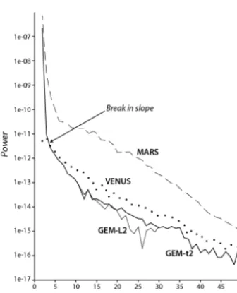
Figure 1. Power spectra for Earth, Venus, and Mars from sets of spherical harmonic coefficients. Earth (solid line) is from GEM-L2 (Lerch et al., 1982) and GEM-t2 (Marsh et al., 1990), Venus (dotted line) is from Nerem et al. (1993), and Mars (dashed line) is from Smith et al. (1993). If the horizontal harmonic degree axis were plotted as a log scale, then the spectra would be nearly a straight line.
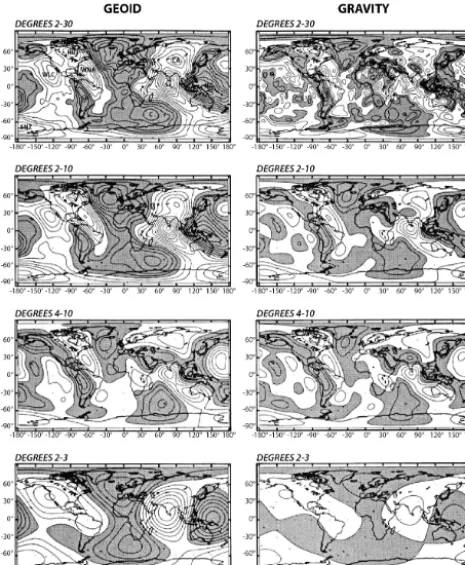
harmonic coefficients of the Goddard Earth Model (GEM) t2 set of coefficients is shown in Fig. 2. That view of the gravi-tational potential field of the Earth has been a puzzle since it was first observed because it shows no correlation with surface continents nor topography, with the single exception of a positive geoid anomaly over the Andes of South Amer-ica (SA). In Fig. 2 note the prominent negative geoid low in the Indian Ocean, the Sri Lanka (SL) Low, and the positive geoid, the New Guinea High (NG). And then in Fig. 3, note that the large summed contributions of degrees 2 and 3 are restricted to only those two NG and SL geoid anomaly sites. In Fig. 3, one can also see that the individual degree contri-butions become decreasingly smaller above degree 10. Thus, we now approach the Earth’s second-largest mass anomaly as it remains buried within the spherical harmonic degree 4–10 packet. Besides illustrating the spatial distribution of the de-gree 4–10 geoid anomalies, Fig. 4 further demonstrates how the large contributions from the degree 2–3 dominate the 2– 10, 2–30, and 2–250 geoid (seen in Fig. 2) fields. Further, Fig. 4 also visually introduces the use of vertical derivatives of the Earth’s potential field into our discussion for resolv-ing Earth structures. In the gravity degree 2–3 map note the paucity of contour lines compared to those in the degree 2– 3 geoid map. Geoid anomalies (1 d−1) are most diagnostic of large mass anomalies at depths of thousands of kilome-ters, whereas gravity anomalies (1 d−2)are most sensitive to mass anomalies within 100 km of the surface.
Figure 2. Earth’s geoid anomaly map for spherical harmonic de-gree ranges 2–250. Computed Goddard Earth Model GEM-t2 coef-ficients (Marsh et al., 1990) are referenced to ellipsoid with recip-rocal flattening of 298.257 (actual Earth flattening).
Figure 3. Magnitudes of individual harmonic degree contributions for the Earth’s 10 major geoid anomaly values computed from the GEM-9 coefficients referenced with reciprocal flattening of 298.257 (actual Earth flattening). Four positive anomalies are New Guinea (NG), Iceland (I), Crozet (C), and South America (SA). Six neg-ative anomalies are Indian Ocean (Sri Lanka) (SL), west of lower California (WLC), central Asia (CA), and south of New Zealand (SNZ). Reprinted from Bowin (1985) with permission.
Consider a site directly over a point mass, the geoid anomaly (N) is
N= V
g0
=GM
g02 ,
where V is the disturbing potential, g0 is normal gravity (9.8 m s−2),Gis the gravitational constant,Mis the anoma-lous mass, andzis the depth of the point mass. The vertical component of gravitygdue to the same point mass is g=GM
Z2 .
The ratio of gravity anomaly to the geoid anomaly directly above the point mass at depthzis then
g N =
Figure 4. Geoid and gravity anomaly maps from GEM-L2 spher-ical harmonic coefficients. Referenced to ellipsoid with reciprocal flattening of 298.257 (actual Earth flattening). Contour intervals are 10 m and 20 mGal, respectively. Degree 2–30 maps obtained by summing contributions from degrees 2 through 30. Degree 2–10, 4–10, and 2–3 maps similarly obtained. In the geoid degree 2–30 map (and in Fig. 2) the 10 major anomalies are labeled, and identi-fied in Fig. 3.
Conversely, the depth can be determined by
Z= g0
g/N.
Then, of course, reentering the value of zinto either, or both, of the point-mass equations for the geoid or gravity can provide estimates of the causative mass. It was by this means that the magnitudes of the mass anomalies of the Earth shown in Fig. 5 were estimated. Two additional verti-cal derivatives of the gravity potential can also aid in defining shallower mass anomaly structures: the vertical gravity gra-dient (1 d−3)and the vertical gradient of the vertical gravity gradient (1 d−4).
For each mass element within the Earth, its geoid contribu-tion falls off as 1 d−1with distance, gravity as 1 d−2, vertical gravity gradient 1 d−3, and vertical gravity gradient of ver-tical gravity gradient 1 d−4. But because all masses within the Earth contribute to all harmonic degrees, it is impossible to invert any one field into its causative masses. However, at selective locations the ratio of gravity anomaly divided by the geoid anomaly value at center locations (Fig. 5) has
Figure 5. Initial estimates of the magnitudes of Earth mass anoma-lies. Estimates are calculated from ratios of gravity anomaly divided by geoid anomaly values at anomaly centers.
already provided constraints on the internal mass anomaly structure of the Earth (Bowin, 1983, 1986, 1991, 2000). At lithospheric subduction sites (positive geoid anomaly band in degree 4–10 map in Fig. 4), the phase changes of olivine and pyroxene grains in the subducted lithosphere are inferred to produce the positive density contrast with the surrounding upper mantle, which forms the second-greatest mass anoma-lies within the Earth (2.0−8×10²²kg).
Figure 6. Percentage contribution curve (CCC) and estimated equivalent point-mass depths for the South American (SA) GEM-t2 geoid high. Depths are estimated from the percentage CCC using spline function coefficients for each degree. Spline functions are from model sets of two and three balanced point masses at depths of 100, 500, 1000, 2900, and 4000 km.
calculating and displaying calculated cumulative contribu-tion curves (CCC) (see, e.g., Bowin (2000), Fig. 12) plotted as percentages of their maximum value, estimates of depths to point-mass sources could be estimated for each potential derivative. The result for the SA geoid high shown in Fig. 6 yielded a consistent point-mass depth of nearly 1200 km depth for all harmonic degrees and all derivatives, indicating a single source as its origin and hence a shallower depth for the actual positive mass anomaly. This 1200 km point-mass depth is also consistent with the SA geoid high source being shallower above the zero contour line at 2900 km depth of the core–mantle topography (Fig. 4, degree 2–3 geoid). This strong evidence for a single source depth for the South Amer-ican geoid high is strong support opposing dynamic topogra-phy as being a significant contributor to the Earth’s geoid.
2 Deriving high derivative Earth potential field model
The gravity field coefficients are estimated with high accu-racy in the long-wavelength part (corresponding to the co-efficients of low degrees). In order to avoid filtering these low degree coefficients, we shift the damping factors above to a certain degree (30) and obtain a new set of filtered co-efficients that have yielded stable estimates of global geoid, gravity, vertical gravity gradient, and vertical gradient of ver-tical gravity gradient anomaly values for degrees 31–264. These coefficients reflect mass anomalies that exist in the outer 200 km of the Earth. Our derived filtered spherical har-monic coefficients for degrees 2–264 are given in the accom-panying Supplement.
Various alternative methods exist for the determination of global gravity field models – such as integration on Earth sphere, least-square adjustment or collocation – and vari-ous data sources are used, such as satellite-based data or terrestrial (surface) observations. The error behaviors of the resulting gravity field models depend on the method, the quality and properties of the observations. In general, the
gravity field is not homogeneously determined. With satel-lite gravimetry the high-frequency part (corresponding to the gravity field coefficients of higher degrees) is computed less accurately than the low-frequency part. This results in some short-wavelength noise in the computed gravity field models. It is therefore necessary to apply filtering to extract the signal by suppressing the accompanying noise.
The idea of filtering gravity field models in the spectral do-main is based on smooth SH coefficients with some depres-sion factors. Various smooth functions have been proposed such as Pellinen (1966) and Jekeli (1981). With a Gaussian mean filter in the spectral domain as an example, as pre-sented by Jekeli (1981), the recursive formula for a Gaussian smoothing coefficients in the spectral domain is given as
β0=1, β1=1+e
−2b
1−e−2b−
1 b, βn=
−2n+3
b βn−1+βn−2, n≥3, whereb= ln 2
1−cos(r/R⊕) withrthe radius of a spherical cap to
be smoothed andR⊕the radius of the Earth.
Using the above filter coefficients, the filtered gravity field coefficients can be derived as
C0 nm S0 nm
=βn
Cnm
Snm
.
The gravity field coefficients are estimated with high accu-racy in the long-wavelength part (corresponding to the coef-ficients of low degrees). In order to avoid filtering these low degree coefficients, we shift the damping factors above to a certain degreen0 and obtain a new set of filter coefficients such that
βn0 =1, n < n0 βn0 =βn−n0, n≥n0.
The gravity field coefficients are estimated with high ac-curacy in the long-wavelength part (corresponding to the co-efficients of low degrees). In order to avoid filtering these low degree coefficients, we shift the damping factors above to a certain degree (30) and obtain a new set of filter co-efficients that have yielded stable estimates of global geoid, gravity, vertical gravity gradient, and vertical gradient of ver-tical gravity gradient anomaly values for degrees 31–264. These coefficients reflect mass anomalies that exist in the outer 200 km of the Earth.
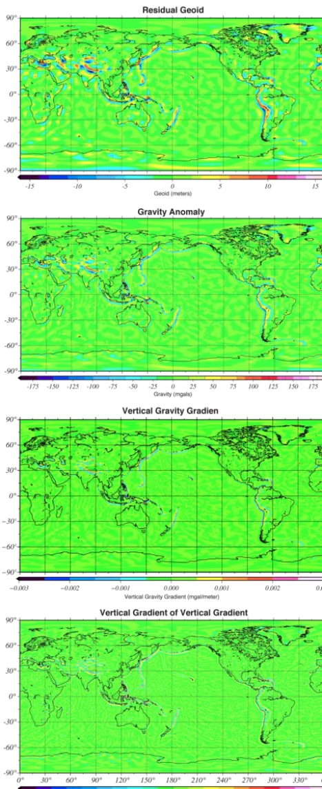
Figure 7. Residual geoid, gravity, vertical gravity gradient, and ver-tical gradient of verver-tical gravity gradient for spherical harmonic de-grees 31–464. Color scale weighted so that each color has same number of data samples.
3 Motions of the Earth’s tectonic plates and earthquakes
In 1960 Harry H. Hess was the first to recognize that the ocean floor was not everywhere ancient (Precambrian) but is, in fact, locally, being created today (Hess, 1960; it was to be published in “The Sea, Ideas and Observations” but became delayed). Robert S. Dietz received a copy of the Hess (1960) preprint and published a paper, Dietz (1961), on seafloor spreading without acknowledging Hess’s prior work. Dietz concluded that ocean basins most likely contained rocks no older than the Mesozoic, and he also noted that linear mag-netic anomalies aligned normal to the presumed flow direc-tion of the presumed convecdirec-tion cells were being found in the Atlantic. Hess then had his paper published in the next avail-able Geological Society of America (GSA) publication vol-ume available, Hess (1962). Magnetic anomaly stripes were reported in the Atlantic Ocean by Vine and Mathews (1963). Wilson (1963) in his Fig. 4 referenced forming the Hawaiian chain over a “stable core of a convection cell” as a possi-ble origin of the Hawaiian chain of islands, whose source later was identified as being to hot spot plumes. Looking back with hindsight, we see a remarkable coming-together of oceanic magnetic anomaly stripes that allowed linkage to normal and reverse paleomagnetic age dating of the oceanic crust beneath, as well as the global patterns of rifts and trans-form faults. And, in turn, aided in the dating of folded and deformed rocks of the former or active subduction collision zones, the depressed sections at rifts, and the horizontal dis-placements along strike-slip faults, like that of the San An-dreas, all fit into the new understanding of plate tectonics and its three types of boundaries. Another consequence of plates rubbing against one another while moving is to in-crease strains in the rocks of the opposing plates, which, when released, cause an earthquake. In this way, the distri-bution of epicenters reveals the locations of plates and their boundaries, as in Fig. 8. However, that figure only displays those having earthquakes having a magnitude 6 or greater; hence the less seismically active borders do not stand out.
Essentially all the analyses of plate motions (Mor-gan, 1973; Soloman and Sleep, 1974; Forsyth and Uyeda, 1975; Chapple and Tullis, 1977) have assumed that plates are not undergoing acceleration. Accordingly, every plate must be in dynamic equilibrium, such that the sum of the torques about any axis must be zero. Previously, the paucity of clear evidence for systematic plate velocity changes through time has led researchers to view convective motion in the mantle, with traction on the overlying litho-sphere, as likely producing plate tectonics, in which plates would move in stages with a terminal velocity. Different stages might have different plate motion direction and/or speed.
Figure 8. Absolute plate velocity vectors (1 per 1000 plotted black arrows) for the 52 plates of Bird (2003) and earthquake locations with magnitudes greater than magnitude 6.0.
that assumption, they formed a spherical triangle amongst the center points of the Hawaiian, Louisville, and Easter Island hotspots. This triangle was then used to identify which digitized location points along the Emperor–Hawaiian seamount chain correlated with which digitized points along the Louisville ridge chain. Then, with those location points correlated in time, they could begin estimating poles of rota-tion. They then took each location point along the Emperor– Hawaiian chain, and bisected its arc with the Hawaii hotspot location and at that bisect point projected a line normal to it. They then did the same procedure to the equivalent point along the Louisville chain with its bend, and where the two normal lines intersect is an equivalent stage pole for that se-lected point. From ages of dredged samples, they estimated Euler poles at 4 and 2 Myr intervals. Figure 9, from Bowin and Kuiper (2005) using the Harada and Hamano (2000) Eu-ler poles, had the Pacific Plate speeding up as it moved north-ward tonorth-ward the Aleutians, then after the bend slowed down, and then again increased speed as it moved towards the Mar-ianas (away from Hawaii).
Bowin (2010) demonstrated that plate tectonics con-serves angular momentum (see Fig. 10) using the 14-major-tectonic-plate history of the Earth (except the Juan de Fuca and Philippine plates). Euler stage pole histories of the past 62 million years of Gripp and Gordon (1990) were given. We believe it is worth restating that “mirroring of the bend in the Emperor–Hawaiian seamount chain in the locations of the 4448 filtered stage pole locations for the absolute mo-tions of the Nazca Plate (Bowin, 2010; Plate No. 11, Fig. 12) gives credence to both the quaternion analyses utilized and the role of impulse in plate motions”. Of the 14 plates ana-lyzed, the Nazca Plate is the only one that has a stage pole pattern revealing such a pronounced bend in stage pole trend at 46 Myr.
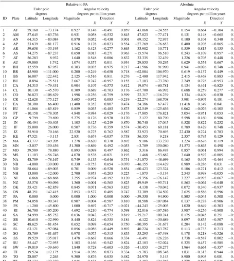
For this present study of active surface deformation we have chosen to use a more detailed 52 tectonic plate model of the Earth’s surface by Bird (2000). Bird’s published Euler pole values are relative to a fixed Pacific Plate. An important contribution was provided by Rick Rosson (Table 1) of Math-works.com, who converted Bird’s 52 relative Euler poles to absolute poles of rotation (Table 1)
Although the rates of plate acceleration/deceleration are very small, they are real and thus indicate that impulse (force times time) due to changes in plate momentums (plate mass times velocity) are what causes deformations within the Earth and on its surface. Thus one of our early tasks was to display the individual plate motion absolute velocity vectors for the 52 plates utilizing the absolute rotation Euler pole data of Table 1 on a global rectangular grid having 5 arcmin spacing (see Fig. 8).
Table 1. Euler pole and angular velocity estimates; based on Pacific Plate absolute rotation from Morgan and Morgan (2007).
Relative to PA Absolute
Euler pole Angular velocity Euler pole Angular velocity degrees degrees per million years degrees degrees per million years ID Plate Latitude Longitude Magnitude Direction Latitude Longitude Magnitude Direction
X Y Z X Y Z
1 AF 59.160 −73.174 0.927 0.148 −0.491 0.859 43.068 −24.555 0.154 0.664 −0.304 0.683 2 AM 57.645 −83.736 0.931 0.058 −0.532 0.845 47.023 −77.471 0.131 0.148 −0.665 0.732 3 AN 64.315 −83.084 0.870 0.052 −0.430 0.901 69.152 72.937 0.100 0.104 0.340 0.935 4 AP 33.639 −81.177 0.916 0.128 −0.823 0.554 −27.269 −76.653 0.400 0.205 −0.865 −0.458 5 AR 59.658 −33.193 1.162 0.423 −0.277 0.863 33.902 10.771 0.559 0.815 0.155 0.558 6 AS 74.275 −87.237 0.650 0.013 −0.271 0.963 −15.574 96.510 0.243 −0.109 0.957 −0.268 7 AT 56.283 8.932 1.640 0.548 0.086 0.832 33.335 32.439 1.226 0.705 0.448 0.550 8 AU 69.080 1.742 1.074 0.357 0.011 0.934 29.853 50.295 0.629 0.554 0.667 0.498 9 BH 12.559 87.957 0.303 0.035 0.975 0.217 −41.586 91.990 0.941 −0.026 0.748 −0.664 10 BR 45.900 −111.000 0.200 −0.249 −0.650 0.718 −62.004 106.970 0.619 −0.137 0.449 −0.883 11 BS 16.007 122.442 2.125 −0.516 0.811 0.276 −2.480 117.942 2.415 −0.468 0.883 −0.043 12 BU 8.894 −75.511 2.667 0.247 −0.957 0.155 −7.103 −73.760 2.249 0.278 −0.953 −0.124 13 CA 54.313 −79.431 0.904 0.107 −0.573 0.812 19.074 −60.781 0.134 0.461 −0.825 0.327 14 CL 10.130 −45.570 0.309 0.689 −0.703 0.176 −67.700 46.992 0.688 0.259 0.277 −0.925 15 CO 36.823 −108.629 1.998 −0.256 −0.759 0.599 22.317 −116.239 1.334 −0.409 −0.830 0.380 16 CR −12.628 175.127 3.605 −0.972 0.083 −0.219 −22.274 168.708 3.901 −0.907 0.181 −0.379 17 EA 28.300 66.400 11.400 0.352 0.807 0.474 24.386 67.477 11.418 0.349 0.841 0.413 18 EU 61.066 −85.819 0.859 0.035 −0.483 0.875 82.549 −125.636 0.062 −0.076 −0.105 0.992 19 FT −10.158 −178.305 4.848 −0.984 −0.029 −0.176 −17.805 176.821 5.054 −0.951 0.053 −0.306 20 GP 9.799 79.690 5.275 0.176 0.970 0.170 2.122 80.790 5.598 0.160 0.986 0.037 21 IN 60.494 −30.403 1.103 0.425 −0.249 0.870 30.740 17.045 0.528 0.822 0.252 0.511 22 JF 35.000 26.000 0.507 0.736 0.359 0.574 −30.453 60.181 0.789 0.429 0.748 −0.507 23 JZ 35.910 70.166 22.520 0.275 0.762 0.587 33.923 70.693 22.430 0.274 0.783 0.558 24 KE 47.521 −3.115 2.831 0.674 −0.037 0.738 36.355 9.218 2.357 0.795 0.129 0.593 25 MA 43.777 149.205 1.278 −0.620 0.370 0.692 9.106 133.230 1.224 −0.676 0.719 0.158 26 MN −3.037 150.456 51.300 −0.869 0.492 −0.053 −3.789 150.080 51.573 −0.865 0.498 −0.066 27 MO 59.589 78.880 0.893 0.098 0.497 0.862 5.316 86.493 0.857 0.061 0.994 0.093 28 MS 11.103 −56.746 4.070 0.538 −0.821 0.193 1.468 −53.682 3.640 0.592 −0.805 0.026 29 NA 48.709 −78.167 0.749 0.135 −0.646 0.751 −51.875 −48.699 0.163 0.407 −0.464 −0.787 30 NB −4.000 139.000 0.330 −0.753 0.654 −0.070 −46.155 114.429 0.989 −0.286 0.631 −0.721 31 ND 58.664 −89.003 0.701 0.009 −0.520 0.854 −60.423 123.324 0.106 −0.271 0.412 −0.870 32 NH 13.000 −12.000 2.700 0.953 −0.203 0.225 −1.873 −3.134 2.543 0.998 −0.055 −0.033 33 NI 6.868 −168.868 3.255 −0.974 −0.192 0.120 −5.356 −176.147 3.227 −0.993 −0.067 −0.093 34 NZ 55.578 −90.096 1.360 −0.001 −0.565 0.825 49.949 −95.741 0.563 −0.064 −0.640 0.765 35 OK 55.421 −82.859 0.845 0.071 −0.563 0.823 4.138 −70.042 0.072 0.340 −0.937 0.072 36 ON 48.351 142.415 2.853 −0.527 0.405 0.747 33.309 134.502 2.625 −0.586 0.596 0.549 37 PA 0.000 0.000 0.000 1.000 0.000 0.000 −59.330 94.900 0.803 −0.044 0.508 −0.860 38 PM 54.058 −90.347 0.907 −0.004 −0.587 0.810 18.588 −107.084 0.137 −0.278 −0.906 0.319 39 PS −1.200 −45.800 1.000 0.697 −0.717 −0.021 −44.243 −25.003 1.020 0.649 −0.303 −0.698 40 RI 36.700 −105.200 4.692 −0.210 −0.774 0.598 32.016 −107.586 3.987 −0.256 −0.808 0.530 41 SA 54.999 −85.752 0.636 0.042 −0.572 0.819 −75.217 100.241 0.175 −0.045 0.251 −0.967 42 SB 10.610 −32.990 8.440 0.824 −0.535 0.184 6.122 −30.689 8.097 0.855 −0.507 0.107 43 SC 48.625 −81.454 0.652 0.098 −0.654 0.750 −80.395 −31.677 0.204 0.142 −0.088 −0.986 44 SL 63.121 −97.084 0.856 −0.056 −0.449 0.892 40.224 163.787 0.113 −0.733 0.213 0.646 45 SO 58.789 −81.637 0.978 0.075 −0.513 0.855 55.293 −67.498 0.178 0.218 −0.526 0.822 46 SS 19.529 135.017 1.478 −0.667 0.666 0.334 −6.491 126.226 1.738 −0.587 0.802 −0.113 47 SU 55.447 −72.955 1.103 0.166 −0.542 0.824 42.103 −52.024 0.325 0.457 −0.585 0.670 48 SW −19.019 −39.640 1.840 0.728 −0.603 −0.326 −41.053 −28.277 1.964 0.664 −0.357 −0.657 49 TI 19.524 112.175 1.514 −0.356 0.873 0.334 −5.783 108.348 1.831 −0.313 0.944 −0.101 50 TO 28.807 2.263 9.300 0.876 0.035 0.482 24.970 5.143 8.980 0.903 0.081 0.422 51 WL 22.134 132.330 1.546 −0.624 0.685 0.377 −3.483 124.268 1.778 −0.562 0.825 −0.061 52 YA 69.067 −97.718 0.998 −0.048 −0.354 0.934 67.697 146.639 0.261 −0.317 0.209 0.925
4 What is going on inside the Earth?
Bowin (2010) demonstrated that it is the sinking of the pos-itive phase change mass anomalies of the subducted litho-sphere that drive plate tectonics. The present locations of those positive mass anomalies are most clearly revealed in the spherical harmonic degree 4–10 coefficient packet of the Earth’s potential field. As the linear bands of subducted
in-Figure 9. Stage pole velocities for Pacific Plate at labeled time on Emperor and Hawaiian seamount chains. From Bowin and Kuiper (2005).
tegration of responses to all internal Earth mass anomalies. However, Fig. 10 suggests that other plates may vary their momentums more rapidly than this Pacific Plate example. Although the resultant momentum Pacific Plate vectors re-mained near constant but had different rates for tens of mil-lions of years during the Emperor and Hawaiian seamount times, the direction changed azimuth by 60◦within about 4 million years.
Figure 10. Angular momentum vs. Myr for 4448 individual filtered plate data over 62–0 Myr of Bowin (2010) and their sum (black cir-cles). Plate ID for plates: AF (Africa, dark grey), AN (Antarctica, dark blue), CA (Caribbean, dark green), CO (Cocos, yellow green), EN (Eurasia, light yellow), IN (India, pale yellow), NA (North America, dark yellow), NZ (Nazca, orange), PA (Pacific, red), and SA (South America, light grey).
Figure 8 provides a present-day sample of how the Earth is behaving after its motion changed from the Emperor seamount chain northward mantle motion era to the Hawai-ian seamount construction era of westward mantle motion. In particular, note that the absolute easterly motion of the di-rection of the Pacific Plate, from the north end of the Tonga trench to the south end of the Yap trench, is essentially at 90◦
to the northerly motion of the adjacent Australian (Au) Plate to the south. An inability to satisfactorily visualize the inter-face between a northern down-going subduction limb of an Australian thermal convection roller cell and a side-slipping transcurrent portion of a Pacific roller thermal-driven con-vection cell led Bowin (2010) to reject that scenario as not being credible. And bear in mind that this geometric setting would have persisted for more than 40 Myr.
Figure 11. Mercator map of oceanic magnetic anomalies and transform faults. Scanned copy of the original 1986 illustration.
Figure 12. World view of deformation index value (1–1000) based on a global topographic grid at 5 arcmin spacing. At each grid location, the maximum relief in meters of the location with the eight adjacent surrounding locations is divided by 5 to obtain its deformation index value.
nearly 36 years later that Bowin (2010) recognized that that beginning of that extension of the South Pacific spreading into the Indian Ocean realm began at the time of the bend in the Emperor–Hawaiian seamount chain (46 Myr). And it ap-pears to have begun with the wedge-shaped opening (spread-ing) of the Tasman Sea off eastern Australia (labeled 2). Then the Pacific Plate spreading progressed southward (2a, 2b), to progressing westward, separating Australia from Antarctica (3a, 3b), and continuing through time to progress westward, moving India northward towards Eurasia, and then opening the Gulf of Aden and hence the Red Sea, to now the Gulf of Aqaba. A southwest-trending branch of a closely spaced young pattern of spreading and transform offsets can also be
seen emanating from the triple-junction point in the Indian Ocean east of Madagascar. This branch coincides with that classified as ultraslow-spreading ocean ridges (Dick et al., 2003).
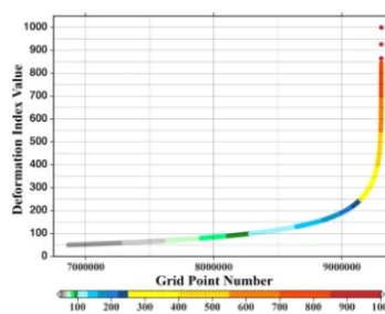
demon-Figure 13. Deformation index values sorted lowest to greatest value vs. sort point number. Note that more than the first 6 million values have values less than 50, and that accounts for the white areas in Fig. 12.
strated that plate tectonic motions are not chaotic. The mo-tions seem rather slow and steady. Even the 60◦ change in azimuth of lithosphere flow that accompanied the “bend” in the Emperor–Hawaiian seamount chain trend near 46 Myr appeared to have not affected the spreading in the Atlantic Ocean, although it did coincide with the beginning of a sig-nificant rearrangement of continents in the Southern Hemi-sphere. The band of positive geoid anomalies in the degree 4–10 packet (Fig. 4, degrees 4–10) shows good agreement with the absolute plate motion vectors for present-day plate motions (Fig. 8), supporting the phase-change conclusion of Bowin (2010). Unfortunately, we cannot satisfactorily esti-mate what the Earth’s spherical harmonic degree 4–10 coef-ficients were for the time period before the bend (say, 90–50 Kyr). Without such a quantitative understanding of a period before the bend with a period after the bend, the best esti-mates of rates of Earth’s internal mass redistributions will remain those of Fig. 4.
We have now become forced to assume the Earth’s spheri-cal harmonic coefficients for degrees 4–10 must change with time to meet the evolving location pattern of dense phase-change subducted lithosphere and periodotic material. Per-haps one should consider that the coefficients for harmonic degrees 2–3 may also evolve with time, and that the locations of the Indian Low (Sri Lanka Low) and New Guinea High lo-cations may also shift with time. But it it appears to be only the smaller mass anomalies of the falling dense masses of the phase change mass anomalies that conserve the angular mo-mentum of the global plate tectonic system. The unanswered question now shifts to the following: how does such a plan-etary system of conservation of angular momentum become activated?
5 Quantifying a deformation index value
Since we can now view “mountain building” deformation as resulting from changes of momentum or impulse, how might
such deformations be quantized? Topographic perturbations from a global mean value are a first-order measure of a de-gree of uplift or subsidence that has occurred in a region, but we sought a deformation index value that would be more rel-evant than simply a local topographic mean or standard devi-ation or a combindevi-ation value. Our selection for this initial test of a deformation index value is to use, at each 5 arcmin pixel, the maximum absolute topographic difference with its eight adjacent neighboring pixels. We used this as a way to esti-mate the absolute maximum local topographic relief value at each grid location as a stand-in for a deformation index value.
Figure 12 presents our first global view of approximately 9 million maximum topographic relief values at 5 arcmin spac-ing usspac-ing a color scale where the topographic relief in me-ters is divided by 5 so that the resulting deformation index value lies between 1 and 1000. Here, in addition to the or-ange and reds associated with the mountainous belts of the Himalayan and Andean ranges, and island arcs of the world, they also locate many of the undersea rises of the southwest Indian Ocean, western Pacific Ocean, and North and South Atlantic mid-ocean rises. And in the northwestern Pacific Ocean basin, a series of non-red nearly east–west-trending, quasi-equally spaced fracture zone features stand out. We are also struck (and puzzled) by the great abundance of yel-low and orange colors from topographic relief in the western central Pacific region. It stands out as a unique part of the world. If deformation index values less than 50 are ignored, and those above 50 are sorted from lowest to highest, then a plot like Fig. 13 results. Figure 13 also helps clarify that over 6 million grid locations in the world map of Fig. 12 have de-formation index values of less than 50 and hence are white on that map.
The Supplement related to this article is available online at doi:10.5194/se-6-1075-2015-supplement.
Acknowledgements. We wish to thank the following for helping us in solving a variety of problems in developing and maintaining functioning computer hardware and software systems: Warren Sass, Christine Hammond, Randy Manchester, Eric Cunningham, Tim Barber, Vladimir Smirov, and Gregory Pike. Jack Cook and Christina Cuellar helped assemble and format convert tables and illustrations, as well as aiding final manuscript preparation. C. O. Bowin thanks the Woods Hole Oceanographic Institution for USD 1500 annual emeritus research support, in 2015 reduced to USD 781. He also thanks the editorial staff and manuscript editor for their support.
References
Bird, P.: An updated digital model of plate boundaries, Geochem. Geophy. Geosy., 4, 1027, 2003.
Bowin, C.: Depth of principal mass anomalies contributing to the Earth’s geoidal undulations and gravity anomalies, Mar. Geod., 7, 61–100, 1983.
Bowin, C.: Global gravity maps and the structure of the Earth, in: The Utility of Regional Gravity and Magnetic Anomaly Maps, edited by: Hinze, W. J., 88–101, Soc. Of Explor. Geophys., Tulsa, OK, USA, 1985.
Bowin, C.: Topography at the core-mantle boundary, Geophys. Res. Lett., 13, 1513–1516, 1986.
Bowin, C.: Earth’s Gravity Field and Plate Tectonics, Tectono-physics issue with contributions to Texas A&M Geodynamics Silver Anniversary Symposium, 187, 69–89, 1991.
Bowin, C.: The geoid and deep Earth mass anomaly structure, in: Geoid and Its Geophysical Interpretations, edited by: Vanicek, P. and Christou, N. T., 343 pp., CRC Press, Boca Raton, FL, USA, 1994.
Bowin, C.: Mass anomaly structure of the Earth, Rev. Geophys., 38, 355–387, 2000.
Bowin, C.: Plate tectonics conserves angular momentum, eEarth, 5, 1–20, doi:10.5194/ee-5-1-2010, 2010.
Bowin, C. and Kuiper, H.: Resolving accelerations of Earth’s Plate tectonics, Poster at AGU Meeting Toronto, Canada, Abstract No. #T43C-01, available at: ftp://ftp.whoi.edu/pub/users/cbowin, 2005.
Bruce, J. G.: Comparison of near surface dynamic topography dur-ing the two monsoons in the western Indian Ocean. Deep Sea Research and Oceanographic Abstracts, Vol. 15, No. 6, Elsevier, Princeton, NJ, USA, 1968.
Chapple, W. M. and Tullis, T. E.: Evaluation of the forces that drive the plates, J. Geophys. Res., 82, 1967–1984, 1977.
Dick, H. J. B., Lin, J., and Schoouten, H.: An ultraslow-spreading class of ocean ridge, Nature, 246, 405–412, 2003.
Dietz, R. S.: Continental and Ocean Basin Evolution by Spreading of the Sea Floor, Nature, 190, 854–857, 1961.
Forsyth, D. and Uyeda, S.: On the relative importance of the driving forces of plate motion, Geophys. J. Roy. Astr. S., 43, 163–200, 1975.
Gripp, A. E. and Gordon, R. R. G.: Current plate velocities relative to the hotspots incorporating the NUVEL-1 global plate motion model, Geophys. Res. Lett. 17, 1109–1112, 1990.
Hager, B. H.: Subducted slabs and the geoid: Constraints on mantle rheology and flow, J. Geophys. Res., 89, 6003–6015, 1984. Hager, B. H. and R. J. O’Connell: A simple global model of plate
dynamics and mantle convection, J. Geophys. Res., 86, 4843– 4867, 1981.
Hager, B. H., Clayton, R. W., Richards, M. A., Comer, R. P., and Dziewonski, A. M.: Lower mantle heterogeneity, dynamic topog-raphy, and the geoid, Nature, 313, 541–545, 1985.
Harada, Y. and Hamano, Y.: Recent progress on the plate motion rel-ative to hotspots, in: The History and Dynamics of Global Plate Motions, Geoph. Monog. Series., 121, 327–338, 2000.
Hess, H. H.: Preprint Evolution Ocean Basins, Princeton Univ. Dept. of Geology, Princeton, NJ, USA, 38 pp., avaiable at: ftp://ftp.whoi.edu/pub/users/cbowinnamedcopy_HHHess_ 1990_evolution_ocean_basins.pdf, 1960.
Hess, H. H.: History of Ocean Basins, in: Petrologic Studies: A Vol-ume in Honor of A. F. Buddington, edited by: Engle, A. E. J., James, H. L., and Leonard, B. F., Boulder, CO, USA, Geological Society of America, 599–620, 1962.
Jekeli, C.: Alternative methods to smooth the earth’s gravity field, project report, The Ohio State University, Ohio, USA, 1981. Lerch, F. J., Klosko, S. M., Laubscher, R. E., and Wagner, C. A.:
Gravity model improvement usig Geos 3 (GEM 9 and 10), J. Geophys. Res., 84, 3897–3916, 1976.
Marsh, J. G., Lerch, F. J., Putney, B. H., Felsentreger, T. L., Sanchez, B. V., Klosko, S. M., Patel, G. B., Robbins, J. W., Williamson, R. G., Engelis, T. L., Eddy, W. F., Chandler, N. L., Chinn, D. S., Kapoor, S., Rachlin, K. E., Braatz, L. E., and Pavlis, E. C.: The GEM-T2 gravitational model, J. Geophys. Res., 95, 22043– 22071, 1990
Morgan, W. J.: Plate motions and deep mantle convection, Geol. Soc. Am. Mem., 123, 7–22, 1973.
Nerem, R. S., Bills, B. G., and McNamee, J. B.: A high resolution gravity model for Venus: GVM-1, Geophs. Res. Lett., 20, 599– 602, 1993.
Pekeris, C. L.: Thermal convection in the interior of the Earth, Mon. Not. R. Astron. Soc., 3, 343–367, 1935.
Pellinen, L. P.: A method for expanding the gravity potential of the Earth in spherical harmonics, Translation ACIC-TC-1282, NTIS: AD-661819, Moscow, Russia, 1966.
Ricard, Y., Richards, M., Lithggow-Bertelloni, C., and Le Stuff, Y.: A geodynamical model of mantle density heterogeneity, J. Geo-phy. Res., 98, 21895–21909,1993.
Soloman, S. C. and Sleep, N.: Some simple physical models for absolute plate motions, J. Geophys. Res., 79, 2557–2564, 1974. Smith, D., Lerch, F. J., Nerem, R. S., Zuber, M. T., Patel, G. B.,
Fricke, S. K., and Lemoine F. G.: An improved gravity model for Mars: Goddard Mars Model 1, J. Geophy. Res., 98, 20871– 20889, 1993.
Vine, F. J. and Matthews, D. H.: Magnetic anomalies over oceanic ridges, Nature, 199, 947–940, 1963.
Wegener, A.: Die Entstehung der Kontinente, Geol. Rundsch., 3, 276–292, 1912 (in German).
Wilson, J. T.: A possible origin of the Hawaiian Islands, Can. J. Phys., 41, 863–870, 1963.