A basing of the diffusion approximation derivation for the four-wave kinetic integral and properties of the approximation

(1)

Nonlinear Processes

in Geophysics

c

European Geophysical Society 2002

A basing of the diffusion approximation derivation for the four-wave

kinetic integral and properties of the approximation

V. G. Polnikov

The State Oceanographic Institute, Kropotkinskii Lane 6, Moscow, 119992 Russia Received: 5 March 2001 – Revised: 23 July 2001 – Accepted: 22 January 2002

Abstract. A basing of the diffusion approximation

deriva-tion for the Hasselmann kinetic integral describing nonlinear interactions of gravity waves in deep water is discussed. It is shown that the diffusion approximation containing the sec-ond derivatives of a wave spectrum in a frequency and angle (or in wave vector components) is resulting from a step-by-step analytical integration of the sixfold Hasselmann integral without involving the quasi-locality hypothesis for nonlinear interactions among waves. A singularity analysis of the inte-grand expression gives evidence that the approximation men-tioned above is the small scattering angle approximation, in fact, as it was shown for the first time by Hasselmann and Hasselmann (1981). But, in difference to their result, here it is shown that in the course of diffusion approximation deriva-tion one may obtain the final result as a combinaderiva-tion of terms with the first, second, and so on derivatives. Thus, the fi-nal kind of approximation can be limited by terms with the second derivatives only, as it was proposed in Zakharov and Pushkarev (1999). For this version of diffusion approxima-tion, a numerical testing of the approximation properties was carried out. The testing results give a basis to use this ap-proximation in a wave modelling practice.

1 Introduction

A kinetic integral for the spectrum evolution rate due to nonlinear interaction among waves derived by Hasselmann (1962) has the kind

∂N (k)

∂t ≡TN(k)=4π Z

dk1

Z dk2

Z dk3 ·M2(k,k1,k2,k3)N (k)N (k1)N (k2)N (k3) ·

₁

N (k)+

1

N (k1) − 1

N (k2) − 1

N (k3)

· δ(σ (k)

+σ (k1)−σ (k2)−σ (k3))δ(k+k1−k2−k3) . (1) Correspondence to: V. G. Polnikov ([email protected])

Here, TN(k) is the nonlinear transfer for the wave action

spectrum,N (k), k is the wave vector andσ (k)is the fre-quency of the same wave component, given by the disper-sion law for deep water of the kindσ_i2 =gki;M(...)is the

four-wave interaction matrix element, andδ(...)is the Dirac delta-function of its argument. It is evident that use of the sixfold integral (1) in its explicit form for the problem of wave evolution is very awkward due to the difficulty of its direct calculation. For this reason, it is rather natural to seek an effective approximation for the integral (1), which retains the main properties of the latter.

Despite a number of attempts to construct approximations for the Hasselmann kinetic integral (see, for example, Has-selmann et al., 1985; Efimov and Polnikov 1991), the regu-lar analytical derivations of approximations are innumerable. Thus, the problem of analytical derivation of an effective ap-proximation for the integral (1) is still important. A recent paper by Zakharov and Pushkarev (1999) can serve as proof of this statement. This circumstance is provided by the prin-cipal role of the kinetic integral for a description of wind wave evolution. From this point of view, a finding of an an-alytical approximation derived by rigorous algebra transfor-mations of Eq. (1) without fitting parameters has a special interest.

At present, in fact, there are only two variants of analyt-ical approximations derived from the exact formula for the kinetic integral (1) on the basis of direct algebra transforma-tions. One of them is derived by

Hasselmann and Hasselmann (1981)1and is called the dif-fusion approximation. The second approximation is derived by Zakharov and Smilga (1981). Later it was conventionally called “the narrow directional approximation” (Zaslavskii, 1989). Here we shall not dwell on the second approxima-tion, noting only that it is applicable for wave spectra with narrow angular spreading functions.

A domain of applicability for the diffusion approximation is more wider. But use of it in the form proposed in paper I

(2)

356 V. G. Polnikov: A basing of the diffusion approximation derivation for the four-wave kinetic integral meets a series of technical difficulties connected to the

calcu-lation of the fourth derivatives for the spectral functionN (k). In this aspect, it seems very interesting to simplify the final expression for the diffusion approximation to a level of the second derivatives forN (k), as it was proposed in Zakharov and Pushkarev (1999)2. Herewith, we should note that their approximation is based on intuitive considerations using the conservation properties of the exact integral (1) but not on algebra transformations of Eq. (1). Therefore, the necessity appears to find the result of paper II by means of direct alge-bra transformations of the integral (1).

In present paper, we make a basing of the diffusion ap-proximation (in terms of a combination of the zero, first, and second derivatives of the spectrumN (k)) by means of con-secutive analytical integration of the integral (1). In this way, we are lucky to find a convenient kind of approximation in the form close to the one proposed in paper II and to give a clear physical treatment to the final result as the small scat-tering angle approximation. We remind the reader that just such a type of diffusion approximation treatment was ini-tially given in paper I. But, in difference to paper I, here it will be shown that there is no necessity to introduce the hy-pothesis of locality for nonlinear interactions among waves, as far as the type of integrand singularities provides itself the small scattering angle approximation. Thus, we are lucky to unite the main ideas of papers I and II.

The structure of the paper is the following. In Sect. 2, following paper I, a short analysis of the diffusion approxi-mation derivation is given. In Sect. 3, the main ideas of the same approximation are discussed, following paper II. An alternative direct derivation of the diffusion approximation is presented in Sect. 4. Section 5 is devoted to a numerical test-ing of the diffusion approximation given in terms of paper II. For this aim, we compare the approximate nonlinear transfer with the numerical results of direct calculations for the inte-gral (1) obtained in Polnikov (1989, 1990). In Sect. 6, the final analysis is carried out and conclusions are drawn.

2 Analysis of the diffusion approximation derivation by Hasselmann and Hasselmann

The main ideas of the diffusion approximation derivation given in paper I are as follows.

1. On the basis of direct calculations of the nonlinear en-ergy transfer,TE(k) ∝ σ−1TN(k), it is proposed that

the main contribution to the transfer is made by the wave components with wave vectorsklocated in the domain k1≈k2≈k3 ≈k(the locality hypothesis for nonlin-ear interactions).

2. The spectra N (k) are expanded in the small vectors, k0 ₌_k

1−k2 andk00 = k3−k. After this, the cubic spectral function under the integral is transformed to an expression containing the second derivatives of spectral 2_{Hereafter is referred to as paper II.}

function in the wave vectors components, and the final integral obtains the form of an integral with respect to the small valuesk0 _and_k00_{, which has a rather strange} mathematical sense.

3. The delta-function for wave vectors is expanded in the same small vectors. As a result, the final expression for the transfer contains the fourth derivatives of the kind

∂N (k)

∂t =

∂2 ∂ki∂kj

Dij lm

"

N2 ∂

2_N

∂ki∂kj

−2N∂N ∂kl

∂N

∂km

#)

, (2)

whereki, kj are the wave vector components, and

Dij lm=2−9

Z Z

(k_l0k_m0 −k_l00k00_m) k_i00k00_jR dk0dk00. (3)

Herewith, the factorRin the integrand (3) contains the frequency delta-function.

4. Using of symmetry properties of the integrand and the conservation laws for the total wave action

A=

Z

N (k) dk, (4)

energy

E=

Z

σ (k) N (k) dk, (5)

and momentum

M=

Z

kN (k) dk (6)

results in an essential simplification of Eq. (2), leading to a decrease in the independent elements number for the tensorDij lm.

5. For the case of deep water, the situation is simplified additionally, as far as there is no need to calculate the integrals (3) directly. Instead, one can use a simple re-lation of the kindDij lm ∝ Cij lmkb with the value b

determined from the dimension consideration. Finally, the expression for the transfer obtains the kind

∂N (k) ∂t =C1

(

∇2+ ∂ 2

∂ki∂kj

kikj

K2

!)

(F1+F2)

+C2

(

2 ∂ 2

∂ki∂kj

kikj

k2

!

F1+

∂2 ∂ki∂kj

F3

+ 2∇2− ∂ 2

∂ki∂kj

kikj

K2

!

F2

)

(3)

where

F1=g 3 2_k

27 2

n

N2∇2N−2N (∇N )2o, (8)

F2=g 3 2_k272

( klkm

k2

N2 ∂

2_N

∂kl∂km

−2N∂N ∂kl

∂N ∂km

) ,(9)

F3=g 3 2_k

27 2

N2 ∂

2_N

∂kl∂km

−2N∂N ∂kl

∂N

∂km

. (10)

The coefficientsC1andC2are determined from a com-parison with exact calculations.

Thus, the derivation in paper I includes the following as-sumptions: one hypothesis (item 2.1), a rather doubtable in-tegral with respect to small variables of the type (3) (item 2.2), and the expansion of the wave vector delta-function, which is not clear in the domain of applicability (item 2.3). All these items decrease the reliability of the final result. Herewith, for justification, one should note that the ideas 2.4. and 2.5. are very fruitful.

Finally, Eq. (7) is the analytical approximation for the inte-gral (1), derived by the rather rigorous, though too sophisti-cated algebra transformations. Its testing carried out in pa-per I showed that this approximation corresponds qualita-tively to the exact one-dimensional energy transfers obtained in paper I by numerical calculations of the integral (1). The approximation (7) reproduces all principal features of the ex-act transfer with the mean error of the order of 30–50% (de-pending on the spectrum shape).

The main drawback of the parameterization (7) is a com-plication of the final formula. In this aspect, the approxima-tion of paper II is more preferable, if it is correctly derived. To check this point, we try to analyze the derivation in pa-per II.

3 Analysis of the diffusion approximation derivation by Zakharov and Pushkarev

The main ideas of the diffusion approximation derivation given in paper II differ absolutely from the ones given in pa-per I. They are as follows:

1. First, the fact of conservation of the total wave action,

A, wave energy,E, and wave momentum,M, is stated as the main feature of the integral (1).

2. Second, there is noted the fact of the exact stationary solutions’ existence for the Eq. (1), including the so-called thermodynamic solution of the kind

N (k)= a

(b+σ (k)), (11)

(where a and b are arbitrary constants) and the Kolmogorov-type solutions of the kind

N (k)∝k−23/6, (12)

N (k)∝k−4, (13)

corresponding to a constant flux of wave action to lower frequencies (the spectrum (12)) and a constant flux of wave energy to higher frequencies (the spectrum (13)). 3. Then, in the polar coordinates, (σ, θ), the simplest

dif-ferential operator of the kind

L= 1 2

∂2 ∂σ2+

1

σ2

∂2

∂θ2 (14)

is constructed, which secures the conservation laws’ va-lidity for valuesA,E, andM. Additionally, this op-erator retains the solution (11), if the initial Eq. (1) is imitated by a model equation of the kind

∂N (k)

∂t =

1

σ3L

₁

N (k)

. (15)

4. In a more general form (taking into account the cubic power of the integrand in the spectral functionN (k), the dimension of the matrix elements, and retention of the Kolmogorov-type solutions), the imitative represen-tation of the kinetic equation obtains the following type of differential equation

∂N (k)

∂t =

c σ3L

N4(k)σ26L

₁

N (k)

. (16)

5. In final form, Eq. (16) is simplified to a second order differential equation of the kind

∂N (k)

∂t =

c0 σ3 L

h

N3(k)σ24 i

, (17)

if one supposes that the spectrum shape is of the kind

N (k) ∝ σ−b8(σ, θ ), where the function 8(σ, θ ) is weakly dependent on frequency. Note that in Eqs. (16) and (17), the dimensional constants,candc0, depend on the gravity acceleration,g.

(4)

358 V. G. Polnikov: A basing of the diffusion approximation derivation for the four-wave kinetic integral

4 Alternative derivation of the diffusion approximation

The main idea of the approach proposed here is based on an analytical part of the numerical calculation algorithm for the integral (1), derived in Polnikov (1989). In accordance with the algorithm mentioned, the analytical transformations are carried out by the following steps.

1. First, both delta-functions under the integral are inte-grated absolutely exact. For this aim, one starts from the integration in the vectork2, which eliminates the wave vector delta-function. Then, a transition to the polar coordinates, (σ, θ ), is carried out, and the exact analytical integration in the angleθ1for the frequency delta-function is executed. As a result, the sixfold inte-gral becomes the threefold one of the kind

∂N (σ, θ )

∂t =c

Z Z Z

M2(...)X_±P3 (18)

N (σ, θ ), N (σ1, θ1), N (σ2, θ₂±),

N (σ1, θ1)

J k2

dσ1dσ3dθ3,

wherecis the dimensional coefficient depending ong,

P3(. . . )is a cubic form of the kind

P3(N , N1, N2, N3)=N1N2(N+N3)

−N N3(N1+N2) , (19) (where, in turn, the following notion is used: Ni =

N (σi, θi), and the zero sub-index is omitted),J is the

Jacobian of the frequency delta-function integration,k2 is the modified wave number corresponding to the point (σ2, θ2±) (see details in Polnikov, 1989).

2. An explicit form ofJ has the kind

J =c0σˆ₂3

ka+k1+ ˆσ22

1/2

ka−k1+ ˆσ22

1/2

h

ka+k1− ˆσ22

1/2

k1+ ˆσ22−ka

1/2i−1 . (20)

wherec0 is the dimensional constant depending ong, and

ˆ

σ2=

σa−σ2 √

g , (21)

σa=σ3+σ =σ1+σ2, (22)

ka=

h

k₃2+k2+2kk3cos(130)

i1/2

, (23)

130≡θ3−θ. (24)

Note that due to the symmetry properties of the inte-grand, integration in Eq. (18) can be restricted by the domain whereσ1 ≤ σ2(i.e. forσ1 ≤ σa/2), while the

value of the constantcis doubled. For the same reason, one can restrict the integral calculation by the condition

σ3≥σwith the same enhancing of the coefficientc.

3. The Jacobian denominator analysis shows that, under the conditionσ3≥σ, integrable singularities arise only due to the factors in the square brackets of the denomi-nator for Eq. (20). By finding the roots of proper equa-tions, one can determine the lower,σ₁(1), and the upper,

σ₁(2), limits for the integral in the variableσ1. Thus, tak-ing into account that said, Eq. (18) can be represented in the kind

∂N (σ, θ )

∂t =C

2π Z 0 dθ3 ∞ Z σ dσ3

σ₁(2)

Z

σ₁(1)

dσ1

M2P3

σ2k2

σ1−σ₁(1) σ+o(130)−σ1

σ3+o(130)−σ1

−1/2

, (25)

where the lower limit is the following

σ₁(1)=σ3σ+o(130)

σ3+σ

(26)

and the upper limit, σ₁(2), is determined by the sec-ond factor in the denominator of Eq. (25). The term

o(130)means that a certain function of the angular dif-ference, 130 ≡ θ3−θ, has a small value for small values of130. Additionally, we should note that, for the values σ3 ≈ σ, the following ratio takes place:

o(130)≈ 0.25(130)2. Thus, the “small scattering an-gle” condition, o(130) 1, is valid up to the values

(130)≈1, i.e. in a rather large interval of the scattering angles.

4. From the structure of Eq. (25) we can draw the follow-ing.

4.1 With a certain accuracy one can assume that a rep-resentative part of the integral is accumulated from the regions of the singular surfaces, i.e. from the re-gions close to the upper and lower limits inσ1 of the integral (25)3. (Exact calculations showed (Pol-nikov, 1995) that the contribution of the singular surfaces is about 25–30% of the total integral and has a proper shape.)

4.2 The main part of the singularity surfaces’ contribu-tion to the integral is given by the singularity at the upper limit,σ₁(2), of the integral inσ1, as far as the singularity has a two-dimensional feature and cor-responds to small values of130and to the condition

σ1≈σ ≈σ3.

4.3 The latter feature corresponds automatically to the criterion of locality for the nonlinear interactions and to the approximation of small scattering angles. 3_{This idea is also used for the stating of approximations in}

(5)

4.4 From that said above, one can draw the main con-clusion that the searched integral can be approxi-mated by an analytical estimation of the contribu-tion at the upper limit of the integral (25) inσ1(i.e. from the region given by the conditions presented in the item 4.4.2.). This estimation is just the small scattering angle estimation. And the locality inter-action condition is merely the consequence of the singularity feature for the integrand, arising with-out involving any hypothesis.

Furthermore, to finish the approximation derivation, one needs to find a regular part of the integrand for Eq. (25) in the vicinity of the most strong singularity (σ1≈σ ≈σ3 ≈σ2,

130 ≈0), which can be denoted by the indexPT, and to execute the rest of the integration. But the cubic formP3(...) at this surface is equal to zero. Therefore,P3(...) should be expanded in a series in frequency and angle at the singularity surface, which leads to arising of the terms of the type in the right-hand side for Eq. (2).

A scheme of analytical transformations is as follows. Re-taining the cubic form under the integral as a separate factor, we have

∂N (σ, θ )

∂t = CM2 6T σ3 2π Z 0 dθ3 ∞ Z σ dσ3

σ₁(2)

Z

σ₁(1)

dσ1P3

6T

·(σ+o(130)−σ1)−1/2(σ3+o(130)−σ1)−1/2.(27)

The Tailor expansion of each spectrum function in the cu-bic formP3at the surface6T is of the kind

N (σi, θi)=N(0)(σ, θ )+Nσ(1)(σi −σ )+0.5Nσ(2)

(σi−σ )2+N_θ(1)(θi−θ )+0.5N_θ(2)(θi−θ )2. . . , (28)

where the mixed derivatives are omitted for simplicity. Sub-stitution of Eq. (28) into Eq. (19), accounting for the reso-nant conditions due toδ-functions under the integral, results in a cancellation of the zero derivatives’ contribution. The left terms with derivatives at the surface6T can be extracted from the integral, which leads to the expression of the kind

∂N (σ, θ )

∂t =

CM2_6T σ3

X

α,β,γ α+β+γ=3

bαβγσ3−β−γ Nσ(0)

α N_σ(1)β

N_σ(2)γ ₊ X

α1,β1,γ1

α1+β1+γ1=3

bα1β1γ1σ

3−β1−γ1 _N(0)

θ

α1

N_θ(1)β1 N_θ(2)γ1 +. . .

(29)

where coefficients bαβγ are the integrals of the following

kind 2π Z 0 dθ3 ∞ Z σ dσ3

σ₁(2)

Z

σ₁(1)

(σ−σ1)β(σ3−σ1)γdσ1

(σ+o(130)−σ1)1/2(σ3+o(130)−σ1)1/2

, (30)

analogous to Eq. (30) with a proper change of variables in the numerator under the integral.

As seen from Eq. (29), the final expression is a sum of terms of the third order in spectral function with different orders of derivatives and with proper coefficients. Thus, the form of the approximation is more general than the one for the diffusion approximation presented in papers I and II. Here we should note that these kind of derivatives depend on the kind of variables. They may be as follows: frequency-angle, wave number modulus–frequency-angle, or wave vector com-ponents. At some conditions (for example, if we use the frequency-angle variables), a contribution of the first deriva-tive terms in Eq. (29) is also cancelled, and the form of the approximation becomes typical to the diffusion one.

The last point of our derivation is to represent the final ex-pression in a compact form, taking into account the conser-vation properties of the initial integral. To do this, it is very convenient to use the ideas 2.4 and 2.5 proposed in paper I. In our case, by analogy, there is no need to carry out the inte-gration in Eq. (30), as far as the dimension considerations are sufficient. In this way, the coefficientsbαβγ in Eq. (29) may

be determined from the conservation laws’ conditions for the total valuesA, E,andM.

Finally, one may expect to obtain an expression similar to Eq. (17), though not in the simplest form proposed in paper II. Particularly, the integration inθ3, taking place in Eq. (25), may lead to a change in the angular dependence of the approximation. But this question deals with a specifica-tion of the diffusion approximaspecifica-tion and is not fundamental at present. The main fact is that, in principal, we have the rigorous derivation of the diffusion approximation for the in-tegral (1).

A specification of the diffusion approximation can be done in the course of consecutive testing more and more compli-cated variants of the approximations. At present, it is worth starting the testing from the variant (17). By determining its advantages and drawbacks, one can move to the direction of a more complicated and more effective analytical approxi-mation in the framework of the result (25), if it is justified in practice.

5 The diffusion approximation testing

(6)

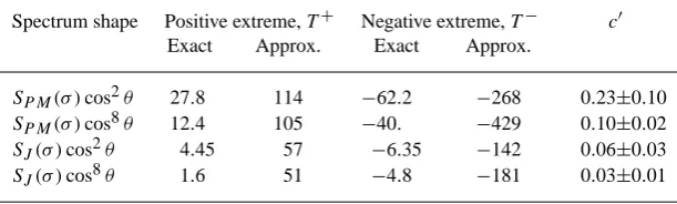
Table 1. Spectrum shapes and calculated nonlinear extremes used for the coefficientc0estimation

Spectrum shape Positive extreme,T+ Negative extreme,T− c0

Exact Approx. Exact Approx.

SP M(σ )cos2θ 27.8 114 −62.2 −268 0.23±0.10

SP M(σ )cos8θ 12.4 105 −40. −429 0.10±0.02

SJ(σ )cos2θ 4.45 57 −6.35 −142 0.06±0.03

SJ(σ )cos8θ 1.6 51 −4.8 −181 0.03±0.01

Note: Estimations forT+andT−are given in units of the coefficient (31). They are found by calculations of the integral (1) (exact) and Eq. (35) (approx.). Estimations ofc0are given by the ratio (exact)/(approx.).

practice. Herewith, the dimensional coefficientc0is changed by a proper, nondimensional one.

Second, a dimensional factor of the kind

c= π 16g

−4_S3

pσ

11

p (31)

is extracted from the final expression for ∂S/∂t, as it was introduced earlier in Polnikov (1989), while tabulating the numerical results for the integral (1) (here,σpandSpare the

peak frequency and the peak value of the spectrum, respec-tively). Thus, by a comparison of approximated and “ex-act” numerical estimations for the transfer∂S/∂t (the latter is presented in Efimov and Polnikov, 1991; Polnikov, 1989), one can easily find the nondimensional coefficient in a trans-formed analytical formula for the diffusion approximation.

Then, a comparison of the two-dimensional transfer for both estimations is carried out, and a quantitative estimation of the approximation error is found. At the final stage, we shall compare a numerical solution of the kinetic equation in the diffusion approximation with the numerical solution of Eq. (1) found in Polnikov (1990).

5.1 Transformation of Eq. (17)

Note that the final formula for the diffusion approxima-tion (17) is very inconvenient for practical use. First, it is not correct in dimension, as the authors proposed in paper II thatg = 1. Second, in Eq. (17), they used the derivatives in frequency and angle, but the wave action spectrum is pre-sented in thek-space. And finally, the wave action spectrum itself does not have its own shape parameterization. This leads to the necessity to use a transformation to the spectrum

S(σ, θ ), whose shape is well-known and widely used. Just for these reasons, Eq. (17) should be rewritten in theS(σ, θ )

representation, at least for the testing problems. Using the definition

N (k)dk= γ g

σ S(σ, θ ) dσ dθ , (32)

whereγ =4π2, it is easy to show that

N (k)= γ g 3

2σ4 S(σ, θ ). (33)

Substitution of Eq. (33) into Eq. (17) gives

∂S

∂t ≡T (σ, θ )= ˜cg

−4_{σ L}h_σ12_S3_{(σ, θ )}i_, ₍₃₄₎ where a proper power ofgand a new, nondimensional coeffi-cientc˜is introduced. Note that the nonlinear energy transfer itself is denoted asT (σ, θ ).

5.2 Nondimensional coefficient estimation

To determine the nondimensional coefficient for the diffusion approximation, let us rewrite Eq. (34) in the kind

T (σ, θ )= π 16g

−4_S3

pσp11c

0 ₁₆

πσ

2

pσ Lˆ

h

ˆ

σ12Sˆ3(σ, θ )i

,(35) wherec0is the sought after coefficient, and the expression in the figure brackets is the modified diffusion operator in which “the hat” means that frequencies and spectra are normalized by their values at the peak point.

As far as the nonlinear transfer, T (σ, θ ) is a two-dimensional function, where a certain procedure of mini-mization should be used to determine a value of the constant

c0. For simplicity, we use the mean value method for estima-tions ofc0obtained by the ratio

c0=T_exa± /T_apr±

for two extreme values of the two-dimensional transfer

T (σ, θ ): the positive extreme,T+, and the negative one,T−. Herewith,T_apr± is calculated by Eq. (35) without coefficient

c0, and is the value tabulated in Efimov and Polnikov (1991) for the cases of direct calculations for the integral (1).

In present calculations the standard JONSWAP shape of the spectrum is used:

S(σ, θ )=Cσ−5exp

−1.25σp

σ 5

·γexp[−(σ−σp)

2_/₀_.₀₁_σ2_]

j 9(θ ) , (36)

where the peak-enhancement parameter,γJ, permits one to

vary the spectrum shape from the Pierson-Moskowitz type,

(7)

V. G. Polnikov: A basing of the diffusion approximation derivation for the four-wave kinetic integral 361

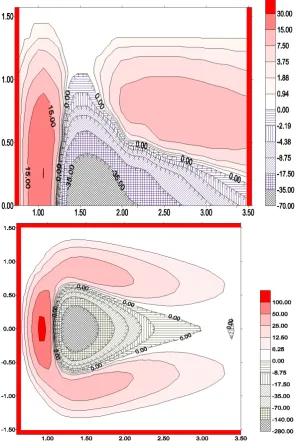
Fig. 1. Two-dimensional nonlinear energy transfers,T (σ, θ ), for the spectrumSP M(σ )cos2θ. (a) A numerical calculation of the integral (1)

from Polnikov (1989) (the upper half of the(σ, θ )– space only); (b) a numerical calculation of the brackets in Eq. (35) (the total(σ, θ )– space). All values are given in units of the dimensional coefficient (31).

(forγJ = 3.3), and9(θ )is the angular spreading function

(for example, see paper I). A value of dimensional coeffi-cient C in Eq. (36) is not significant for our calculations, due to normalization of the spectrum bySp, as it was

men-tioned above. Calculated valuesT+andT−for the approx-imated and exact variants, in units of the constantcgiven by Eq. (31), are presented in Table 1, for a series of the spectrum shapes.

From Table 1 it follows:

(1) The coefficientc0 is not constant, and its value varies depending on the spectrum shape;

(2) The dependence mentioned is enhancing while the

derivatives of the spectrum function are increasing; (3) The united estimation of c0 for all types of spectral

shapes cannot be found with reasonable accuracy. Thus, it should be determined with a preferable spectral shape. For practical use of the approximation, it is preferable to choose a spectral shape following from the numeri-cal solution of the kinetic equation. The latter is close to the typical JONSWAP spectral shape (see Polnikov (1990)). In such case, the following estimation of the coefficientc0can be accepted:

(8)

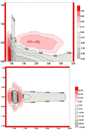
Fig. 2. Two-dimensional nonlinear energy transfers,T (σ, θ ), for the spectrumSJ(σ )cos8θ. See legend in Fig. 1.

An adequacy extent of the estimation obtained can be established by way of comparison of the numerical so-lutions for Eqs. (1) and (34).

5.3 Analysis of a two-dimensional energy transfer topology

A topology of two-dimensional nonlinear energy transfer for exact and approximate calculations was compared, both for the spectra presented in Table 1 and for the other more complicated spectral shapes (including two-mode and non-symmetrical shapes). A series of two-dimensional transfers are shown in Figs. 1, 2, and 3.

Analysis of the total set of calculations permits one to draw the following. First, the approximate two-dimensional trans-fer has a topology close to the exact one. Namely:

– the main extremes,T+andT−, have almost the same values and locations in the (σ, θ)-space;

– local extremes exist as well, but their locations are

shifted remarkably;

– for nonsymmetrical spectral shapes, locations and

val-ues of the main extremes,T+ andT−, are reasonably accurate;

– for two-mode spectra, only locations of the main

(9)

V. G. Polnikov: A basing of the diffusion approximation derivation for the four-wave kinetic integral 363

fig3a

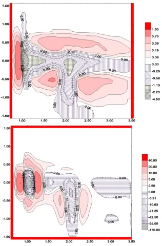
Fig. 3. Two-dimensional nonlinear energy transfers,T (σ, θ ), for the two-mode and nonsymmetrical spectrum from Polnikov (1989) of the kindSJ(σ, σpl=1)cos8θ+0.8SJ(σ, σpl=2)cos4(θ+π/4).

Second, both types of estimations are quantitatively more closer to each other for the spectra with less stronger deriva-tives in frequency and angle (for example, of the type

SP M(σ )cos2θ). But such type of spectra are not similar to

a numerical solution of the kinetic equation, and the estima-tion of c0 of the kind (37) is chosen for the other spectral shapes. Therefore, a mean accuracy of the approximate es-timation for the two-dimensional transfer is of the order of 50%. Just this fact is taken into account for the error interval in the estimation (37).

Nevertheless, as a whole, one may state a rather good cor-respondence of the approximation (35) to the exact transfer, taking into account a lack of any fitting parameters (to say

nothing about the coefficientc0). 5.4 Numerical solution of Eq. (34)

As it was mentioned above, the final conclusion about dif-fusion approximation effectiveness can be drawn on the ba-sis of comparison of the numerical solutions for Eqs. (1) and (34). For Eq. (1), the proper solutions are known from Polnikov (1990). Following this paper’s investigation logic, let us find numerical solutions for Eq. (34), taking the initial spectra from Table 1.

(10)

fig3a

Fig. 4. Two-dimensional nonlinear energy transfers,T (σ, θ ), for the two-mode and nonsymmetrical spectrum from Polnikov (1989) of the kindSJ(σ, σpl=1)cos8θ+0.8SJ(σ, σpl=2)cos4(θ+π/4).

σ_p−1(0) (σp (0)) is the peak frequency of the initial

spec-trum, usually having the valueσp(0) = 1). The spectral

shape becomes close to a universal (self-similar) one, de-pending weakly on an initial spectral shape. Therefore, to estimate the approximation effectiveness, we have to com-pare some representative spectral parameters for solutions of Eqs. (1) and (34) at the evolution timet > τ.

In Polnikov (1990), the following features for the self-similar spectral shape were revealed:

a) the one-dimensional spectrum,S(σ ), has a tail fall law of the kindS(σ )∝σ−n, with the valuen=7±1 at the

frequenciesσ > σp;

b) the frequency width,δ, defined by the relationship

δ=

Z

S(σ ) dσ /S(σp)σp, (38)

has a small varying value of the order ofδ = 0.25± 0.03;

c) the angle narrowness at the peak frequency,Dp, defined

(11)

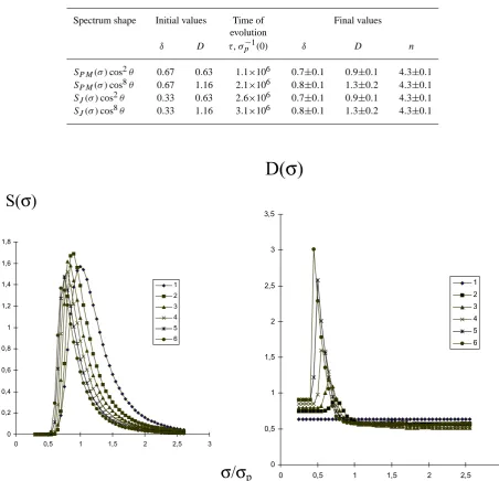
Table 2. Estimations of the spectrum parameters at large evolution time scales

Spectrum shape Initial values Time of Final values evolution

δ D τ, σ_p−1(0) δ D n

SP M(σ )cos2θ 0.67 0.63 1.1×106 0.7±0.1 0.9±0.1 4.3±0.1

SP M(σ )cos8θ 0.67 1.16 2.1×106 0.8±0.1 1.3±0.2 4.3±0.1

SJ(σ )cos2θ 0.33 0.63 2.6×106 0.7±0.1 0.9±0.1 4.3±0.1

SJ(σ )cos8θ 0.33 1.16 3.1×106 0.8±0.1 1.3±0.2 4.3±0.1

S(

_σ

)

σ

/

_σ

p

Fig. 4a.

0 0,2 0,4 0,6 0,8 1 1,2 1,4 1,6 1,8

0 0,5 1 1,5 2 2,5 3 1 2 3 4 5 6

D(

_σ

)

σ

/

_σ

p

Fig. 4b.

0 0,5 1 1,5 2 2,5 3 3, 5

0 0,5 1 1,5 2 2,5 3

1 2 3 4 5 6

Fig. 5. One-dimensional spectrum shape evolutionS(σ, t )(panel (a)) and angular narrowness functionD(σ, t )(panel (b)) at six moments in time (in units,σp−1(0)): 1−t=0, 2−t=7.5×103, 3−t=38×103, 4−t=111×103, 5−t=257×103, 6−t=502×103. Initial

spectrum isSP M(σ )cos2θ.

θp, by the relationship

D(σp)≡D=S(σp, θp)/

Z

S(σp, θ ) dθ, (39)

has a small varying value of the order ofDp =1.05±

0.05.

Thus, the criterion of diffusion approximation quality is an extent of the proper parameters’ closeness to the values given above at the evolution timet > τ ∼=(105−106)σ_p−1(0).

Let us not dwell on technical details of a numerical solu-tion for Eq. (34), but rather let us discuss the results for the

mentioned parameters presented in Table 2 for the evolution timet > τ ∼=106σ_p−1(0).

As seen from Table 2, the spectral shape parameters ob-tain more or less constant values which can be estimated as follows

n=4.3±0.1, (40)

δ=0.75±0.2, (41)

Dp=1.1±0.3. (42)

(12)

366 V. G. Polnikov: A basing of the diffusion approximation derivation for the four-wave kinetic integral it differs remarkably from one inherent to the numerical

so-lution for Eq. (1). Details of the difference between these self-similar shapes are rather numerous. As an example, the numerical solution result for Eq. (34), with an initial two-dimensional spectrum of the kindSP M(σ )cos2θ, is shown

in Fig. 4 in terms of the one-dimensional spectrum,S(σ ), and the angular narrowness function,D(σ ). But, as one can see, this difference is not so fundamental with respect to the fact of self-similar spectral shape existence.

To our mind, these testing calculations are sufficient for a testing investigation of the diffusion approximation proper-ties.

6 Results analysis and conclusions

Thus, on the basis of a step-by-step analytical integration procedure, we were lucky to find mathematical grounds for the diffusion approximation of the Hasselmann kinetic inte-gral in the form proposed in paper II. Herewith, we did not in-volve the locality hypothesis for nonlinear interaction among gravity waves. This property follows from the features of res-onance surface singularities for the four-wave interactions, the contribution of which, to the integral, is assumed to be representative.

Given the example of the approximation (34), it was shown that this diffusion approximation variant secures cor-rectly a geometry of the two-dimensional transfer,T (σ, θ ), not only for simple spectral shapes,S(σ, θ ), but also for com-plicated ones as well (namely two-mode and angular non-symmetric ones). The mean error of the approximated esti-mation forT (σ, θ )is of the order of 50%, for the total set of the spectra considered. This accuracy level is provided by the principal features of the differential form of the ap-proximation, a quality of which decreases with an increase in spectrum derivatives.

The presented examples of the kinetic equation solutions, found in the diffusion approximation of the kind (34), have shown that the spectrum evolution is similar to one for a nu-merical solution of Eq. (1), including the fact of self-similar spectral shape existence at large time scales. But the scat-tering of the self-similar spectral shape parameters is greater, and their values differ from ones for the numerical solutions of Eq. (1). For this approximation the self-similar spectra are more wider in frequency and more narrower in angle, in general.

Taking into account the qualitative likelihood of the two-dimensional spectrum evolution in the diffusion approxima-tion (34), one may draw the conclusion about a possible use

of this approximation for practical forecasting of windwaves, when the error of input data is rather great due to its own na-ture. Herewith, one should take into account that a numerical model fitting, as a rule, diminishes significantly the system-atic error created by separate model elements.

In order to elaborate on the diffusion approximation, one could use the possibility to improve the angular (and fre-quency also) part of the diffusion operator for the nonlinear transfer by way of a better specification for the cubic spectral term under the integral in Eq. (25), taking into account the expansion Eq. (29).

Acknowledgement. The author is thankful to V. Zakharov, V. Kra-sitskii, and I. Kabatchenko for a stimulating interest to this work. The study was partially supported by the Russian Foundation for Basic Research, project # 99–05–64236.

References

Efimov, V. and Polnikov, V.: Numerical modeling of wind waves, Kiev. Naukova dumka Publishing House, 1991.

Hasselmann, K.: On the non-linear energy transfer in a gravity wave spectrum. Pt.1. General theory, J. Fluid Mech., 12, 481– 500, 1962.

Hasselmann, S. and Hasselmann, K.: A symmetrical method of computing the nonlinear transfer in a gravity wave spectrum, Hamburger Geophys. Einzelschrift., Heft 52, 1981.

Hasselmann, S., Hasselmann, K., Allender, K. J., and Barnett, T. P.: Computations and parameterizations of the nonlinear energy transfer in a gravity-wave spectrum. Part II, J. Phys. Oceanogr., 15, 1378–1391, 1985.

Polnikov, V. G.: Calculation of the nonlinear energy transfer through the surface gravity waves spectrum, Izv. Acad. Sci. SSSR, Atmos. Oceanic. Phys., (English transl.) 25, 118–904, 1989.

Polnikov, V. G.: Numerical solution of the kinetic equation for sur-face gravity waves, Izv. Acad. Sci. USSR, Atmos. Ocean. Phys., (English transl.) 26, 118–123, 1990.

Polnikov, V. G.: The study of nonlinear interactions in a wind wave spectrum, Doctor of sciences dissertation, Sevastopol, (in Rus-sian) 1995.

Zakharov, V. E. and Smilga, A. V.: On quasi-one-dimensional spec-tra of weak turbulence, Sov. Phys. JETP, (English spec-transl.) 54, 701–710, 1981.

Zakharov, V. E. and Pushkarev, A.: Diffusion model of interacting gravity waves on the surface of deep fluid, Nonlin. Proc. Geo-phys., 6, 1–10, 1999.