SRef-ID: 1607-7946/npg/2004-11-505
Nonlinear Processes
in Geophysics
© European Geosciences Union 2004
Cross wavelet analysis: significance testing and pitfalls
D. Maraun and J. Kurths
Department of Physics, Potsdam University, D-14415 Potsdam, Germany
Received: 13 August 2004 – Revised: 5 November 2004 – Accepted: 8 November 2004 – Published: 11 November 2004 Part of Special Issue “Nonlinear analysis of multivariate geoscientific data – advanced methods, theory and application”
Abstract. In this paper, we present a detailed evaluation of
cross wavelet analysis of bivariate time series. We develop a statistical test for zero wavelet coherency based on Monte Carlo simulations. If at least one of the two processes con-sidered is Gaussian white noise, an approximative formula for the critical value can be utilized. In a second part, typi-cal pitfalls of wavelet cross spectra and wavelet coherency are discussed. The wavelet cross spectrum appears to be not suitable for significance testing the interrelation between two processes. Instead, one should rather apply wavelet co-herency. Furthermore we investigate problems due to multi-ple testing. Based on these results, we show that coherency between ENSO and NAO is an artefact for most of the time from 1900 to 1995. However, during a distinct period from around 1920 to 1940, significant coherency between the two phenomena occurs.
1 Introduction
Time series analysis is a fundamental issue in climatology as in many other fields of empirical research (von Storch and Zwiers, 1999; Ghil et al., 2002). Considering climate records one almost always faces a composition of numerous scales ranging from days to decades or even longer periods. The classical method to investigate such data by frequency decomposition is Fourier analysis (Priestley, 1992; Brock-well and Davis, 1987). On the considered time scales cli-mate processes are often non-stationary and time resolved methods become necessary. The straightforward time re-solved extension of Fourier analysis is a windowed or slid-ing Fourier Transformation (Kaiser, 1994). A disadvantage of this method is, that the window width and thus the time resolution is constant for all investigated frequencies. Here, continuous wavelet analysis (Daubechies, 1992) has proven to be superior: The time resolution is intrinsically adjusted
Correspondence to: D. Maraun
to the scales. Thus optimal time resolution for every scale is given. Another advantage of wavelet analysis is the flexible choice of the mother wavelet according to the characteristics of the investigated time series (in the following, we always omit the term “continuous”). For an introduction to discrete wavelet transformation and its applications see Kaiser (1994) and Percival and Walden (2000).
During the last decade, wavelet analysis has been success-fully applied in climate science, e.g. to El Ni˜no/Southern Os-cillation (ENSO) data (Gu and Philander, 1995; Kestin et al., 1998; Torrence and Webster, 1998), NAO proxy data (Ap-penzeller et al., 1998) or output of globally coupled ocean at-mosphere models (Timmermann et al., 1999). A good intro-duction to the basic theory and application of wavelet anal-ysis is given by Torrence and Compo (1998). The most im-portant contribution of the latter paper is developing detailed significance tests for the wavelet power spectrum to address the critics, that wavelet analysis is rather producing colorful images than reliable results.
An important field in time series analysis, especially in climate sciences, is multivariate analysis. When compar-ing two different variables like temperature or pressure, or when analyzing teleconnections, one needs the bivariate ex-tension of wavelet analysis. This cross wavelet analysis, which was introduced by Hudgins et al. (1993) and oth-ers, is briefly discussed by Torrence and Compo (1998). It has already been applied to various problems in climatol-ogy like the ENSO-Monsoon system (Torrence and Webster, 1999), ENSO-North Atlantic Oscillation (NAO) teleconnec-tions (Huang et al., 1998), a rainfall-runoff cross analysis (Labat et al., 2000) or the influence of NAO on European surface temperatures (Pozo-Vazquez et al., 2001).
−0.8 −0.6 −0.4 −0.2 0 0.2 0.4 0.6 0.8
−3 −2 −1 0 1 2 3
Amplitude
Time
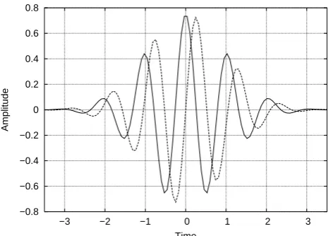
Fig. 1. Real (solid line) and imaginary (dashed line) part of the Morlet wavelet withω0=6.
modeled by Gaussian white noise, we present an approxima-tive formula to easily calculate the critical value for signifi-cance on the 95% level. A second focus of the paper are typi-cal pitfalls of cross wavelet analysis. We show, that not every structure in a wavelet plot has got a physical meaning but might be an artefact of WCS or multiple testing. To illustrate our discussion, we show that the coherency between ENSO and NAO for most of the moderate and strong El Ni˜nos be-tween 1900 and 1995 as suggested by Huang et al. (1998) is an artefact of WCS. However, during a distinct period from around 1920 to 1940 significant coherency between the two phenomena occurs and invites to further investigation.
The paper is organized as follows: In Sect. 2 we intro-duce the most important measures for wavelet analysis. The problem of normalizing wavelet spectra is briefly explained in Sect. 3. In Sect. 4, we interpret wavelet analysis as an in-verse problem of parameter estimation and discuss the con-sequences arising. Sect. 5 provides a numerical significance test for time- and scale-dependent coherency. Important pit-falls related to cross wavelet analysis are studied in Sect. 6. We review the cross wavelet analysis of ENSO and NAO in Sect. 7.
2 Definitions
2.1 Continuous wavelet transformation
The wavelet transformationWi(s)at timeti=i1ton a scale
s of a discrete time series xj=x(tj) of length N with a
sampling interval 1t can be interpreted as an extension of the discrete Fourier transformationF (ω)=P
jxjexp(iωtj)
(Kaiser, 1994). The latter one extracts contributions on fre-quencyω. Wavelet transformation replaces the periodic ex-ponential exp(iωtj) with a localized wavelet 9(tj−ti, s),
which is located around the timeti and stretched according
to the investigated scales: Thus the time series can be de-composed scale- and time-dependent:
Wi(s)= N−1 X
j=0
xj9((j−i)1t, s). (1)
If one considers arbitrary scales between the sampling inter-val and the length of the time series, one speaks of continuous wavelet transformation (CWT). In this case, the wavelets do not span an orthogonal set of basis functions. Hence neigh-boring scales and times contain redundant information and are correlated.
The wavelet9(tj−ti, s)is a stretched and translated
ver-sion of a chosen mother wavelet, normalized with a factor
c(s)(see Sect. 3):
9(tj−ti, s)=c(s)90 t
j −ti
s
. (2)
2.2 Morlet wavelet
In the following, we always consider the Morlet mother wavelet (see Fig. 1)
90(θ )=π−1/4eiω0θe−θ
2/2
, (3)
where θ and ω0 are unit-less. The Gaussian envelope exp(−θ2/2) localizes the wavelet in time. The time/scale resolution is adjusted byω0. For high values ofω0, the scale resolution increases, whereas time resolution decreases and vice versa. Fourier frequencyf and wavelet scales are not direct reciprocals of each other. Instead, one has to rescale the result of wavelet analysis with a factor depending on the mother wavelet (Meyers et al., 1993; Torrence and Compo, 1998). For the Morlet wavelet, the conversion reads
1
f =
4π s ω0+
q 2+ω02
. (4)
For ω0=6, s·f is approximately one. For other mother wavelets refer to Kaiser (1994) and Torrence and Compo (1998).
2.3 Wavelet power spectrum
Transferring a concept of Fourier analysis, a wavelet power spectrum (WPS) can be defined as the wavelet transforma-tion of the autocorrelatransforma-tion functransforma-tion. Following the Wiener-Khinchin theorem, this can be implemented as follows:
WPSi(s)= hWi(s)Wi(s)∗i. (5)
The brackets denote expectation values. WPSi(s)describes
the power of the signalx(t )at a certain timeti on a scales.
2.4 Cross wavelet analysis
As in Fourier analysis, the univariate WPS can be extended to compare two time seriesx(ti)andy(ti): One can define
the wavelet cross spectrum WCSi(s)as the expectation value
of the product of the correspondingWix(s)andWiy(s):
WCSi(s)= hWix(s)W y i (s)
∗i
. (6)
In Sect. 6 we show, that WCS-peaks can even appear when
x(ti)andy(ti)are independent, because WCS is not
normal-ized. In contrast to the WPS, the WCS is complex valued (analogous to Fourier cross spectra) and can be decomposed into amplitude|WCSi(s)|and phase8i(s):
WCSi(s)= |WCSi(s)|ei8i(s). (7)
The phase8i(s)describes the delay between the two signals
at timetion a scales.
A normalized time and scale resolved measure for the relationship between two time seriesx(ti) andy(ti)is the
wavelet coherency (WCO), which is defined as the amplitude of the WCS normalized to the two single WPS:
WCOi(s)=
|WCSi(s)|
WPSxi(s)WPSyi(s)1/2
. (8)
A value of 1 means a linear relationship betweenx(ti)and
y(ti)around timeti on a scales. A value of zero is obtained
for vanishing correlation. Because of the normalization, spu-rious peaks can occur for areas of low wavelet power. Note the importance of estimating the expectation values of the single terms in Eq. (8): If they are not considered separately, nominator and denominator equal each other and the result will be identical to 1 no matter what the real WCO is. Thus computing WCO from observational data, one has to smooth nominator and denominator separately (see also Sect. 4.2).
3 Normalizations
In Fourier analysis, any normalization automatically pro-vides the following two features:
– The Gaussian white noise spectrum is (by definition)
flat.
– Sines of the same amplitude have the same integrated
power in the frequency domain.
In wavelet analysis, we meet difficulties to obtain both. For the factorc(s)in Eq. (1), Torrence and Compo (1998) and Kaiser (1994) suggest different normalizations, which only preserve one of the mentioned features. Torrence suggests
c(s)=
1t s
1/2
, (9)
which preserves a flat white noise spectrum, but sines of equal amplitude exhibit different integrated power propor-tional to their oscillation scale. This choice equals Kaiser’s normalization withp=1/2 (Eq. 3.5 in Kaiser, 1994, p. 62).
1 2 3 4
1 2 4 8
Power
Scale
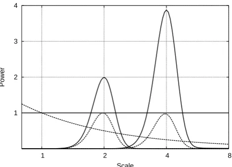
Fig. 2. Wavelet power spectrum of Gaussian white noise and two
sines of frequency 1/2 and 1/4 and equal amplitude. Solid line: Nor-malization according to Torrence and Compo (1998) does not pre-serve the integrated power, but a flat white noise spectrum. Dashed line: Normalization according to Kaiser (1994) preserves the inte-grated power, but the white noise spectrum is∼1/scale.
Using the normalization of Kaiser withp=0,
c(s)=1t1/2, (10)
sines of equal amplitude also exhibit equal integrated power (when scale is plotted logarithmically). On the other hand, the white noise spectrum is no longer flat but decreases pro-portional to 1/scale. Figure 2 illustrates this dilemma of dif-ferent normalizations for time series of Gaussian white noise and a sine function.
Fortunately, the normalization is only relevant for a first inspection by eye. A normalization following Eq. (9) em-phasizes power on high scales and could lead to misinterpre-tations. However, when performing a significance test, the significance level already includes the chosen normalization.
4 Wavelet analysis of observational records
4.1 The inverse problem
4.2 Estimator for wavelet power
The observed WPS of a measured time series is an estimator for the “true” WPS of the underlying process. A comparison with Fourier analysis illustrates the involved consequences:
For the Fourier spectrum, the first guess estimator is the periodogram, which is the squared absolute value of the Fourier transformation of a given time series (Priestley, 1992; Brockwell and Davis, 1987). If this time series is a re-alization of a mixing process, every value of the periodogram isχ2distributed with two degrees of freedom. The variance of this estimator will not converge to zero for an infinite time series, i.e. the periodogram is not a consistent estimator. To construct a consistent estimator for the true spectrum, one has to estimate the expectation value of the periodogram. In many practical cases, when only one realization is given, this has to be done by smoothing neighboring frequencies.
This line of argumentation can be transferred to wavelet analysis: Commonly, as an estimator for the true WPS, the squared absolute value of the CWT is calculated (i.e. Eq. 5 without taking the expectation value). This measure is called wavelet periodogram (Nason et al., 2000) to emphasize that it is like the Fourier periodogramχ2-distributed with 2 degrees of freedom and thus not a consistent estimator. This does not contradict the finding of Percival and Walden (2000), who state that the global wavelet spectrum is a consistent estima-tor of the time independent spectrum. There the expectation value is estimated by averaging over all times.
In wavelet analysis, the situation is quite subtle: Since neighboring points in time and scale are correlated (see Ap-pendix A), the wavelet periodogram looks smooth. However, fluctuations around the true WPS are not smaller as in Fourier analysis, but vary jointly. Hence, the appearance of smooth patterns can suggest structures which are just coincidence. This has to be kept in mind, when interpreting wavelet plots. Ideally, the expectation value should be estimated. When, as usually in climatology, only one realization is measured, one either has to assume stationarity over a certain time in-terval and smooth in time direction, or one has to assume that neighboring scales exhibit similar power and thus smooth in scale direction (Sect. 5). For WCO the smoothing is essen-tial, as shown in Sect. 2.4.
4.3 Edge effects
The wavelet transformation at a point in timet0always con-tains information of neighboring data points. The number of these points depends on the chosen wavelet and the scale considered. Thus, if the wavelet is centered close to the be-ginning or the end of the time series, edge effects occur. The area, where such effects are relevant, is called the cone of influence. Here, the results should be interpreted carefully. In the figures of this paper, the cone of influence is chosen as thee-folding time of the Morlet wavelet
√
2sand marked as a shadow in the wavelet plot. For a discussion, refer to Torrence and Compo (1998).
5 Significance testing of wavelet coherency
The wavelet transform of the realization of a mixing process is a random number. Thus, even for independent processes, nonzero values of the coherency will result and the question arises, when a value has to be considered as being different from zero. The idea is to formulate a null hypothesis H0“the processes are not coherent” and to derive a significance test for H0. Therefore, one has to estimate the probability dis-tribution of the coherency under H0. If the coherency lays outside a chosenα-quantile, the so-called critical value of this distribution, one rejects H0 and the coherency is con-sidered to be significantly different from zero on the(1−α) -level. For an introduction to significance testing refer to Hon-erkamp (1994), Lehmann (1986) or Cox and Hinkley (1994). In the case of Fourier analysis, a test for significant co-herency can be calculated straightforwardly (Brockwell and Davis, 1987): Irrespective of the two processes to be ana-lyzed, the Fourier transform is asymptotically Gaussian dis-tributed and thus the cross periodogram is χ2 distributed. Since vicinal frequencies are asymptotically uncorrelated, the coherency thus follows a F distribution.
However, this is not the case for different wavelet scales and times. Firstly, for small scales the asymptotic – process independent – distribution is not reached. Thus, consider-ing small scales, one has to find suitable models for the two processes to be analyzed. Secondly, vicinal wavelet times and scales are not uncorrelated (Appendix A) and we show in Appendix B, that the WCS is notχ2distributed. Thus an analytical test statistic is highly non trivial if not impossible. To overcome the second problem, we performed Monte Carlo simulations to estimate the distribution under H0 nu-merically. We first considered the most basic case: We simu-lated 10 000 realizations of two independent Gaussian white noise processes and estimated the 95% critical values for dif-ferent smoothing windows in time and scale and for vari-ous time/scale resolutions defined byω0. Since WCO is a local and normalized measure, instationarity of the investi-gated process does not require instationary models to derive the test statistics.
Given a choice of the smoothing window in time and scale, a scale independent critical value is desirable to ease the anal-ysis (since white noise is stationary in time, the critical value will automatically be time independent). We found that this is obtained for the following smoothing procedures:
– When smoothing in time direction, one has to take into
account the wavelet length of essential support, which is proportional to the scalesconsidered (see Eq. 3). Thus, a scale independent critical value is obtained, when the smoothing length is related to the actual scale s by a constant factorm.
– Given a wavelet transform calculated for scales which
are equidistant in logarithmic scale (i.e. more values for smaller scales), one has to smooth a constant number
(a)
1.0000
0.9998
0.9996
0.9994
0.9992
0.9990
0.9988
0.9986
6 12 24 48 96 192 384
95%−Quantile
Scale [∆t]
m=1
m=2
m=3
(b)
0.8 0.82 0.84 0.86 0.88 0.9 0.92 0.94 0.96 0.98 1
6 12 24 48 96 192 384
95%−Quantile
Scale [∆t]
2w+1=11
2w+1=21
2w+1=31
2w+1=41
2w+1=61
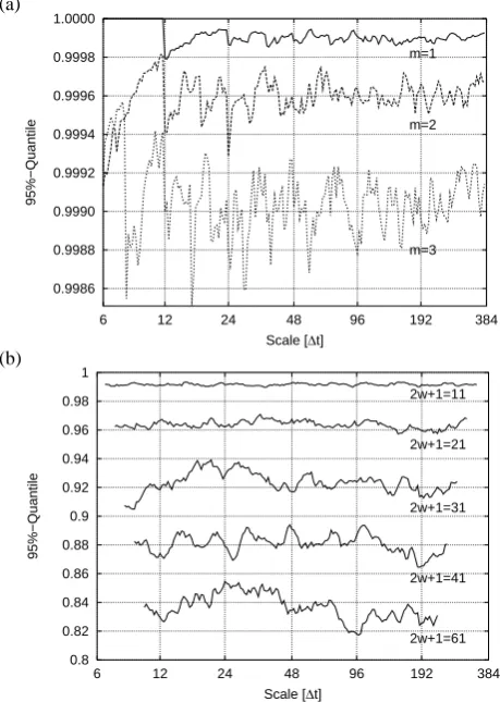
Fig. 3. Empirical 95% critical values for 10 000 realizations of wavelet coherency of two white noise time series forω0 = 6 and for smoothing with different smoothing window lengths (a) in time direction and (b) in scale direction. mdenotes the ratio between window length and scale. 2w+1 denotes the window lengths in relation to the 200 scales, chosen equidistant in logarithmic scale between 61tand 3841t, i.e. 0.5 and 32 years for the common case of1t=1 month. For everymandw, the estimated value fluctuates around a time independent constant.
Figure 3 presents the 95% critical values WCO95 obtained from the Monte Carlo simulations of two Gaussian white noise models. We use the Morlet wavelet and a fixedω0=6 for different smoothing windows in (a) time direction and (b) scale direction respectively. The efficiency of smoothing is rather weak due to the strong correlation between neigh-boring times and scales (see Appendix A). Furthermore, smoothing in time direction appears to be much less effective than smoothing in scale direction (compare the values at the ordinates). This finding becomes intuitively clear, when we recall that wavelets already intrinsically smooth in time di-rection. As expected, we found the normalization discussed in Sect. 3 having no influence on the significance test, since different normalizations cancel down in WCO.
The dependency of WCO95 for the two Gaussian white noise models on the relevant parametersω0and the smooth-ing length in scale directionwis shown in Fig. 4. The plotted values for WCO95are the mean values over all scales of the
3
6
9
12
ω0
0 5 10
15 20 25 w
0.65 0.70 0.75 0.80 0.85 0.90 0.95 1.00 95%−Quantile
Fig. 4. Empirical 95% critical values for 10 000 realizations of wavelet coherency of two Gaussian white noise time series for smoothing in scale direction with different smoothing window lengthswand differentω0. The plotted quantiles WCO95are the mean values over all scales plotted in Fig. 3b, but for variousω0.
Monte Carlo simulations for a fixed pair of parametersω0 andw as depicted forω0=6 in Fig. 3b. For practical pur-poses, we fitted a polynomial to these results and obtained the following approximation for significance testing WCO using the Morlet wavelet and smoothing in scale direction:
WCO95 =8.23×10⁻⁵ω03 +4.24×10 −5ω2
0w +1.13×10⁻⁵ω
0w2+1.54×10⁻⁵w3 −2.30×10⁻³ω02 −2.19×10⁻³ω0w −7.51×10⁻⁴w2 +2.05×10⁻²ω0 +1.27×10⁻²w +0.95,
(11)
where 2w+1 denotes the width of the smoothing window andω0defines the time/scale resolution. This approximation is only valid in the interval shown in Fig. 4. Since smoothing in time direction appears to be too ineffective, we did not consider it in detail.
(a)
period [years]
time [years]
1860 1880 1900 1920 1940 1960 1980 2000 1
2
4
8
16
32
(b)
period [years]
time [years]
1860 1880 1900 1920 1940 1960 1980 2000 1
2
4
8
16
32
Fig. 5. Contour plot of the amplitude of (a) WCS and (b) WCO (2w+1=31) between NINO3 time series and a Gaussian white noise time series. ω0=6. (a) Contours with arbitrary units in log-arithmic scale. Even though the processes are independent, mis-leading peaks appear for high NINO3 values. (b) Linear grey scale from black (WCO=0) to white (WCO=1). The black contour line denotes WCO95. The structure suggested in the wavelet cross spec-trum disappears and thus turns out to be an artefact. Only spurious peaks due to multiple testing (see Sect. 6.2) remain. The shadow marks the cone of influence (see Sect. 4.3).
6 Pitfalls
6.1 Peaks in wavelet cross spectra
WCS describes the common power of two processes without a normalization to the single WPS. This can produce mis-leading results, because one essentially multiplies the CWTs of two time series. E.g. if one of the spectra is locally flat and the other exhibits strong peaks, this can produce peaks in the cross spectrum, which may have nothing to do with any relation of the two time series. Thus, WCS is not suitable for significance testing the relation between two time series. Figure 5 exemplifies the problem showing the WCS between the NINO3 time series (see Sect. 7) and a realization of a first order auto regressive (AR[1]) process. Although both
100 90 80 70 60 50 40 30 20 10 0
Time 0.5
1
2
4
8
16
32
Scale
Fig. 6. 95% critical value contour plot for wavelet coherency of two independent white noise time series. The solid line denotes smoothing with 2w+1=11 points, the dashed line with 2w+1=41 points in scale direction. Even though the two processes are in-dependent, peaks covering around 5% of the time/scale area will appear by definition due to multiple testing
processes are independent by definition, a structure related to the peaks in the NINO3 WPS (i.e. El Ni˜nos) occurs (Fig. 5a). WCO avoids this problem by normalizing to the single WPS (Fig. 5b). However, if one has detected a significant interre-lation using WCO, one can apply WCS to estimate the phase spectrum.
6.2 Multiple testing
When performing a test on the(1−α)-level, by definition one rejects H0 with a probability of α% even when it is true. Hence when repeating a test for many independent realiza-tions, aroundα% of the results should spuriously appear to be significant. This effect is referred to as multiple testing (Lehmann, 1986). Significance testing for WCO can also be seen as an example for multiple testing, since one investi-gates every point in the space/time domain separately. The important difference to a setting with independent realiza-tions is the fact, that neighboring realizarealiza-tions are correlated according to Appendix A and due to smoothing.
on the Bonferroni correction. If a single peak covers more than 5% of the total area, the question is answered easily. For peaks with smaller area, a valuable hint is given in Fig. 6: For different smoothing lengths, spurious peaks do not always overlap. Thus one should always compare different smooth-ing windows and sort out peaks that appear only in one of the corresponding plots. Additionally, it seems that the size of the considered patches plays an important role, as small structures appear much more often than larger ones. One could investigate the distribution of the peak areas under H0 to draw more distinct conclusions about single peaks. This issue is beyond the scope of this paper.
7 Cross wavelet analysis of ENSO/NAO teleconnections
A prominent example of a bivariate time and scale resolved study is the WCS analysis of the ENSO-NAO teleconnec-tions by Huang et al. (1998), stating that ENSO and NAO are coherent for most of the moderate and strong El Ni˜nos be-tween 1900 and 1995. Keeping in mind the discussion in the previous section, we review the WCS results and compare them with those of WCO. We used the extended NINO3-index updated from Kaplan et al. (1998) and the NAO-NINO3-index defined in Jones et al. (1997). We consideredN=1738 data points in the range from January 1856 to October 2000 in a monthly resolution.
Figure 7a shows the results of the WCS analysis (ω0=6). As in the analysis of Huang et al. (1998), several peaks ap-pear at a period of about six years around 1877, 1918 and 1940, and at a period between 2 to 4 years around 1888, 1969 to 1982. All these peaks are associated with El Ni˜no Events. However, a significant peak in the WCS might simply arise due to a peak in the univariate WPS of one of the time series as shown in Sect. 6.1. Thus we additionally calculated the normalized WCO (see Fig. 7b,ω0=6, 2w+1=31) and com-pared it to the WCS. For the calculation of the critical value, we chose Eq. (11). This critical value matches the result of additional Monte Carlo simulations, using an AR[1] process with ane-folding time of 12 months to model NINO3 and Gaussian white noise to model NAO. For WCO, most peaks from the WCS analysis vanish. However, this analysis shows significant peaks around 1920 at a scale of 4 to 8 years and around 1940 at a scale of about 4 to 14 years. The other small peaks cannot be distinguished from coincidence due to multiple testing.
These results cast doubt on the finding that ENSO and NAO are coherent for most of the moderate and strong El Ni˜nos between 1900 and 1995. However, the period between around 1920 and 1940 seems to be distinct from other times, as a significance coherency occurs. The physical interpreta-tion of this time-dependent interrelainterpreta-tion requires further de-tailed investigation of possible instationary coupling mecha-nisms.
(a)
period [years]
time [years]
1860 1880 1900 1920 1940 1960 1980 2000 1
2
4
8
16
32
(b)
period [years]
time [years]
1860 1880 1900 1920 1940 1960 1980 2000 1
2
4
8
16
32
Fig. 7. Contour plot of the amplitude of (a) WCS and (b) WCO (2w+1=31) between NINO3 and NAO index time series. ω0=6. (a) Contours with arbitrary units in logarithmic scale. The WCS (not smoothed) shows peaks around 1877, 1888, 1918, 1940, 1969 and 1982. (b) Linear grey scale from black (WCO=0) to white (WCO=1). The black contour line denotes WCO95. WCO analysis reveals that only a peak around 1920 at a scale of 4 to 8 years and one around 1940 at a scale of about 4 to 14 years are significant.
8 Conclusions
In this paper we present a detailed evaluation of cross wavelet analysis. We investigate two wavelet measures for the linear scale and time dependent interrelation between two time se-ries, the wavelet cross spectrum (WCS) and the normalized wavelet coherency (WCO). The latter one exhibits values be-tween zero and one, characterizing a vanishing or perfect lin-ear relationship respectively. Based on an inverse problem point of view, we recall that the wavelet periodogram is not a consistent estimator of the local wavelet power spectrum (WPS) and that the inference of peaks from wavelet analysis is not unambiguous. Particularly with regard to WCO, one has to estimate expectation values to get any reliable results. In practical cases, this has to be done by smoothing.
re-quired to decide, whether a WCO-value has to be consid-ered as being significantly different from zero. In contrast to Fourier analysis, this test is not independent of the structure of the two processes considered and not easily calculated an-alytically. Instead, appropriate models have to be chosen and Monte Carlo simulations have to be performed to estimate critical values for a chosen significance level. We exempli-fied this discussion for the basic case of two processes which can be modeled by Gaussian white noise. The critical value
WCO95is essentially a function of the smoothing parameters and the time/scale resolution defined byω0. An interesting result is that due to correlations of neighboring scales and times, smoothing has only a weak effect. Especially smooth-ing in time direction is not feasible. For practical purposes, we fitted a polynomial to our numerical results. The critical values derived for the two Gaussian white noise models and thus the approximation Eq. (11) are valid, if at least one of the processes considered can be modeled by Gaussian white noise. For other cases, appropriate models have to be chosen to perform Monte Carlo simulations.
A second focus of the paper are pitfalls of cross wavelet analysis. We show that the WCS can show misleading peaks even for realizations of independent processes, just because the WPS of one of the time series exhibits strong peaks. Thus, WCS is not suitable for significance testing the inter-relation between two processes and one should rather utilize WCO. Furthermore, due to multiple testing spuriously sig-nificant peaks have to appear by definition. A straightfor-ward identification of a single peak is only possible, when this peak covers a percentage of the investigated time/scale area higher than the significance level. For the decision, if a small single peak is significant, no straightforward solution exists so far. However, a valuable hint is given by comparing the peak for different WCO parameters as smoothing length and time/scale resolution.
On the basis of these results, we could show that the sug-gested coherency between ENSO and NAO for most of the moderate and strong El Ni˜nos between 1856 and 2000 is an artefact. The peaks visible in the WCS rather stem from high power in the single WPS of the NINO3 time series than from any coherency of the two time series. The WCO analysis shows significant peaks only around 1920 at a scale of 4 to 8 years and between 1920 and 1940 at a scale of about 4 to 14 years.
Summarizing the discussion in this manuscript, we recom-mend the following steps for cross wavelet analysis:
– Choose suitable models for the significance test of
WCO. If at least one of the models is Gaussian white noise, the approximation Eq. (11) can be used to calcu-late critical values for a chosen significance level. Oth-erwise, Monte Carlo simulations have to be performed.
– Choose the time/scale resolution ω0 (better compare different values).
– Calculate WCO and plot a contour line at the critical
value.
– Check the result of different smoothing lengths. If peaks
appear only for single smoothing lengths, they are prob-ably artefacts due to multiple testing.
However, further research is required. Understanding how the critical value for significant WCO depends on the stochastic models used to describe the investigated processes, could help to avoid time intensive Monte Carlo simulations. An important issue is the treatment of multiple testing ef-fects. To our knowledge, there is no standard procedure for a test, that is not too conservative, but does not produce many false positive results. It seems that the area of the investi-gated peaks in the time/scale domain plays an important role, as small structures appear much more often than larger ones. Thus one could try to estimate the size distribution of spu-riously significant patches to draw more distinct conclusions about single peaks.
Appendix A Correlation of wavelet scales and times
In Fourier analysis, for a white noise time series neighbor-ing frequencies are uncorrelated. Here we show that this is no longer the case for wavelet analysis. Given a continuous white noise time seriesx(t ), the continuous formulation of Eq. (1) reads
W (s, t )= Z ∞
−∞
dτ 90(τ −t )x(τ ), (A1)
where two different points in time are uncorrelated:
hx(t1) x(t2)i =δ(t1−t2). (A2) The correlation between the CWT of two different scaless1 ands2at different timest1andt2is defined as
C(s1, s2, t1, t2)= hW (s1, t1) W (s2, t2)∗i. (A3) Inserting Eq. (A1) into Eq. (A3), we obtain
C(s1, s2, t1, t2)= *
Z Z
dτ1dτ290(τ1−t1)
90(τ2−t2)x(τ1) x(τ2) +
. (A4)
Since integrals and expectation values are linear operators, this can be simplified to
C(s1, s2, t1, t2)= Z Z
dτ1dτ290(τ1−t1)
90(τ2−t2) D
x(τ1) x(τ2) E
. (A5)
Using Eq. (A2) and some algebra lead to
C(s1, s2, t1, t2)= r
2s1s2 s12+s22exp
iω0s1+s2
s12+s22(t2−t1)
× exp
−1 2
(t2−t1)2+ω20(s2−s1)2 s12+s22
. (A6)
Appendix B Distribution of the cross wavelet spectrum
A condition for a simple analytical test statistic for Fourier coherency is based on the fact, that the cross spectrum ex-hibits aχ2distribution (Brockwell and Davis, 1987). Since we have shown that wavelet times and scales are not uncor-related, this condition is no longer trivially fulfilled.
The theorem of Ogasawara and Takahashi (c.f. Rao (1965)) states, when a sum of squares of correlated Gaus-sian distributed random variables isχ2distributed. Given a vector Y of Gaussian random variables
Y∼Nn(0, 6) (B1)
with a covariance matrix6, the product YTAY isχ2 dis-tributed, when
6A6A6=6A6 (B2)
holds.
In the case of smoothing neighboring values of the WCS, we are interested in the sum of squares (in this example smoothing over three neighboring scales is considered. Gen-eralization follows straight forward)
YTAY=W1(s1)W2(s1)∗ +W1(s2)W2(s2)∗
+W1(s3)W2(s3)∗. (B3) This relation is obtained by defining
Y=
W1(s1)
W2(s1)∗
W1(s2)
W2(s2)∗
W1(s3)
W2(s3)∗ (B4) and A=
0 1 0 0 0 0 0 0 0 0 0 0 0 0 0 1 0 0 0 0 0 0 0 0 0 0 0 0 0 1 0 0 0 0 0 0
. (B5)
The covariance matrix then reads
6=
σ 0 σ12 0 σ13 0 0 σ 0 σ12 0 σ13
σ12 0 σ 0 σ23 0 0 σ12 0 σ 0 σ23
σ13 0 σ23 0 σ 0 0 σ13 0 σ23 0 σ
(B6)
where the single entries can be calculated according to Eq. (A6). For these conditions, Eq. (B2) reads
0 0 0 0 0 0 0 0 0 0 0 0 0 0 0 0 0 0 0 0 0 0 0 0 0 0 0 0 0 0 0 0 0 0 0 0
=
0 s1213 0s1213230s131223
0 0 0 0 0 0
0s1213230 s1223 0s231213
0 0 0 0 0 0
0s1312230s2312130 s1323
0 0 0 0 0 0
(B7)
withsij kl=σ2+σij2+σkl2 and sij klmn=2σ σij+σklσmn and is
never fulfilled. Thus the smoothed WCS is not χ2 dis-tributed.
Acknowledgements. We thank M. Kallache, U. Schwarz, M. Rosenblum and A. Pikovsky for inspiring discussions. Our special thanks are dedicated to R. Dahlhaus, who called our attention to the theorem of Ogasawara and Takahashi. D.M. was funded by Deutsche Forschungsgemeinschaft, SFB 555. J.K. was supported by SPP 1114.
Edited by: M. Thiel Reviewed by: two referees
References
Anger, G.: Basic Principles of Inverse Problems, in Inverse Prob-lems: Principles and Applications in Geophysics, Technology and Medicine, Akademie Verlag, 1993.
Appenzeller, C., Stocker, T., and Anklin, M.: North Atlantic oscil-lation dynamics recorded in Greenland ice cores, Science, 282, 446–449, 1998.
Brockwell, P. and Davis, R.: Time Series: Theory and Methods, Springer, 1987.
Cox, D. and Hinkley, D.: Theoretical Statistics, Chapman & Hall, 1994.
Daubechies, I.: Ten Lectures on Wavelets, Society for Industrial and Applied Mathematics, 1992.
Ghil, M., Allen, M., Dettingern, M., Ide, K., Kondrashov, D., Mann, M., Robertson, A., Saunders, A., Tian, Y., Varadi, F., and Yiou, P.: Advanced Spectral Methods for Climate Time Series, Re-views of Geophysics, 40, 3/1–3/41, 2002.
Gu, D. and Philander, S.: Secular changes of annual and interannual variability in the Tropics during the past century, J. Climate, 8, 864–876, 1995.
Honerkamp, J.: Stochastic Dynamical Systems, VCH, 1994. Honerkamp, J.: Statistical Physics, Springer, 1998.
Huang, J., Higuchi, K., and Shabbar, A.: The relationship between the North Atlantic Oscillations and El Ni˜no-Southern Oscilla-tion, Geophys. Res. Lett., 25, 2707–2710, 1998.
Hudgins, L., Friebe, C., and Mayer, M.: Wavelet Transforms and Atmospheric Turbulence, Phys. Rev. Lett., 71, 3279–3282, 1993. Jones, P., J´onsson, T., and Wheeler, D.: Extension to the North Atlantic Oscillation using early instrumental pressure observa-tions from Gibraltar and South-West Iceland, Int. J. Climatol., 17, 1433–1450, 1997.
Kaiser, G.: A friendly Guide to Wavelets, Birkh¨auser, 1994. Kaplan, A., Cane, M., Kushnir, Y., Clement, A., Blumenthal, M.,
and Rajagopalan, B.: Analyses of global sea surface temperature 1856–1991, J. Geophys. Res., 103, 18 567–18 589, 1998. Karlin, S. and Tylor, H.: A first course in stochastic processes,
Aca-demic Press, 1975.
Kestin, T., Karoly, D., Yang, J., and Rayner, N.: Time-frequency variability of ENSO and stochastic simulations, J. Climate, 11, 2258–2272, 1998.
Labat, D., Ababou, R., and Mangin, A.: Rainfall-runoff relations for karstic springs. Part II: continuous wavelet and discrete or-thogonal multiresolution, J. Hydrol, 238, 149–178, 2000. Lehmann, E.: Testing Statistical Hypothesis, Springer, 1986. Meyers, S., Kelly, B., and O’Brien, J.: An introduction to wavelet
the dispersion of Yanai waves, Mon. Wea. Rev., 121, 2858–2866, 1993.
Moritz, H.: General Considerations Regarding Inverse and Related Problems, in Inverse Problems: Principles and Applications in Geophysics, Technology and Medicine, Akademie Verlag, 1993. Nason, G., von Sachs, R., and Kroisandt, G.: Wavelet processes and adaptive estimation of the evolutionary wavelet spectrum, J. Roy. Stat. Soc. B, 62, 271–292, 2000.
Percival, D. and Walden, A.: Wavelet Methods for Time Series Analysis, Cambridge Univ. Press, 2000.
Pozo-Vazquez, D., Esteban-Parra, M., Rodrigo, F., and Castro-Diez, Y.: A study of NAO variability and its possible non-linear influ-ences on European surface temperature, Clim. Dynam., 17, 701– 715, 2001.
Priestley, M.: Spectral Analysis and Time Series, Academic Press, 1992.
Rao, C.: Linear Statistical Inference and its Applications, Wiley Series in Probability and Mathematical Statistics, 1965. Timmermann, A., Latif, M., Grotzner, A., and Voss, R.: Modes
of climate variability as simulated by a coupled general circu-lation model. Part I: ENSO-like climate variability and its low-frequency modulation, Clim. Dynam., 15, 605–618, 1999. Torrence, C. and Compo, G.: A practical guide to wavelet analysis,
Bull. Amer. Meteor. Soc., 79, 61–78, 1998.
Torrence, C. and Webster, P.: The annual cycle of persistence in the El Ni˜no Southern Oscillation, Quart. J. Roy. Met. Soc., 124, 1985–2004, 1998.
Torrence, C. and Webster, P.: Interdecadal Changes in the ENSO-Monsoon System, Journal of Climate, 12, 2679–2690, 1999. von Storch, H. and Zwiers, F.: Statistical Analysis in Climate