Formulation of scale transformation in a stochastic data assimilation framework

https://doi.org/10.5194/npg-24-279-2017 © Author(s) 2017. This work is distributed under the Creative Commons Attribution 3.0 License.

Formulation of scale transformation in a stochastic

data assimilation framework

Feng Liu1,3and Xin Li1,2,3

1_{Key Laboratory of Remote Sensing of Gansu Province, Northwest Institute of Eco-Environment and Resources,} Chinese Academy of Sciences, Lanzhou 730000, China

2_{Center for Excellence in Tibetan Plateau Earth Sciences, Chinese Academy of Sciences, Beijing 100101, China} 3_{University of Chinese Academy of Sciences, Beijing 100049, China}

Correspondence to:Xin Li ([email protected])

Received: 11 June 2016 – Discussion started: 30 June 2016

Revised: 20 April 2017 – Accepted: 3 May 2017 – Published: 15 June 2017

Abstract. Understanding the errors caused by spatial-scale transformation in Earth observations and simulations re-quires a rigorous definition of scale. These errors are also an important component of representativeness errors in data assimilation. Several relevant studies have been conducted, but the theory of the scale associated with representative-ness errors is still not well developed. We addressed these problems by reformulating the data assimilation framework using measure theory and stochastic calculus. First, mea-sure theory is used to propose that the spatial scale is a Lebesgue measure with respect to the observation footprint or model unit, and the Lebesgue integration by substitution is used to describe the scale transformation. Second, a scale-dependent geophysical variable is defined to consider the het-erogeneities and dynamic processes. Finally, the structures of the scale-dependent errors are studied in the Bayesian frame-work of data assimilation based on stochastic calculus. All the results were presented on the condition that the scale is one-dimensional, and the variations in these errors depend on the differences between scales. This new formulation pro-vides a more general framework to understand the represen-tativeness error in a non-linear and stochastic sense and is a promising way to address the spatial-scale issue.

1 Introduction

The spatial scale in Earth observations and simulations refers to the observation footprint or model unit in which a geo-physical variable is observed or modelled (scale is used

be-low as an abbreviation for spatial scale). Scale is tradition-ally defined in terms of distance, which is not adequate both because distance is a one-dimensional quantity while scale generally refers to a two- or three-dimensional space and because the scale may change in a very complicated man-ner (for example, from an irregular observation footprint to a square observation footprint). Generally, the scale is not explicitly expressed in the dynamics of a geophysical vari-able, partially because a rigorous definition of scale is dif-ficult to find, except for an intuitive conception (Goodchild and Proctor, 1997) and certain qualitative classifications of scale (Vereecken et al., 2007). This reflects the complexity of scale and consequently requires a more rigorous mathe-matical conceptualisation of scale.

The scale transformation of a geophysical variable may re-sult in significant errors (Famiglietti et al., 2008; Crow et al., 2012; Gruber et al., 2013; Hakuba et al., 2013; Huang et al., 2016; Li and Liu, 2017; Ran et al., 2016). These errors are mainly caused by the strong spatial heterogeneities (Miralles et al., 2010; Li, 2014) and irregularities (Atkinson and Tate, 2000) that are associated with geophysical variables across different scales, and are also closely related to dynamic vari-ations, e.g. in hydrological (Giménez et al., 1999; Vereecken et al., 2007; Merz et al., 2009; Narsilio et al., 2009), soil (Ryu and Famiglietti, 2006; Lin et al., 2010) and ecological (Wiens, 1989) processes. How to elucidate the scale transfor-mation by developing mathematical tools has yet to be fully addressed.

gener-alised framework in Earth system modelling and observation (Talagrand, 1997). Geophysical data are typically observed by various Earth observations; thus, updating the observation data in a data assimilation system may result in scale trans-formations between the observation space and system state space. If observation operator is strongly non-linear and com-plex, the errors caused by the scale transformation are even more serious (Li, 2014). An important concept that is re-lated to the scale transformation in data assimilation is “rep-resentativeness error”, which is associated with the inconsis-tency in the spatial and temporal resolutions between states, observations and operators (Lorenc, 1986; Janji´c and Cohn, 2006; van Leeuwen, 2014; Hodyss and Nichols, 2015), and the missing physical information that is related to a numer-ical operator compared to the ideal operator (van Leeuwen, 2014), such as the discretisation of a continuum model or neglect of necessary physical processes. The representative-ness error and instrument error make up the observation error of data assimilation. Under the Gaussian assumption, they are independent of each other (Lorenc, 1995; van Leeuwen, 2014). This study will not consider the instrument error when formulating the scale transformation in data assimilation.

Recently, approaches have been developed to assess the representativeness error. Janji´c and Cohn (2006) studied the representativeness error by treating system state as the sum of resolved and unresolved portions. Bocquet et al. (2011) used a pair of operators, namely, restriction and prolonga-tion, to connect the relationship between the finest regular scale and a coarse scale, and determined the representative-ness error using a multi-scale data assimilation framework. van Leeuwen (2014) considered two complicated cases, i.e. conducting the observation vector in a finer resolution com-pared with system state vector and assimilating the retrieved variables. Their solutions were formulated using an agent in observation or state space, and a particle filter was pro-posed to treat the non-linear relationship between observa-tions, states and retrieved values. Hodyss and Nichols (2015) also estimated the representativeness error by investigating the difference between the truth and the inaccurate value that is generated by forecasting model.

Although these approaches explored the structure of the representativeness error and offered various solutions, im-provements are still necessary to investigate the exact ex-pression of the errors caused by scale transformation in data assimilation. The authors believe that these approaches are optimal in linear systems but may not be suitable when ob-servations are heterogeneous and sparse, or when operators are non-linear between states and observations, although the general equations in the non-linear case were given. With-out taking heterogeneities and non-linear operators into ac-count, the representativeness error cannot be fully under-stood. However, heterogeneity varies depending on the sit-uation and is difficult to formulate in a general theoretical study.

Data assimilation studies based on stochastic processes (Apte et al., 2007; Miller, 2007) or a stochastic dynamic model (Miller et al., 1999; Eyink et al., 2004) have been pro-posed recently. Compared to deterministic models, stochas-tic data assimilation is more applicable in an integrated and time-continuous theoretical study (Bocquet et al., 2010) and creates an infinite sampling space of the system state (Apte et al., 2007). Although the theorems of calculus that are based on stochastic processes (or stochastic calculus) are different from those of ordinary calculus, these advantages suggest that stochastic data assimilation offers a more general frame-work to study scale transformation.

We attempt to explore the mathematic definitions of scale and scale transformation, and then formulate the errors caused by the scale transformation on stochastic data assim-ilation in a general theoretical study. The next section in-troduces the basic concepts and theorems of measure the-ory, stochastic calculus and data assimilation. In Sect. 3, we present the definitions of scale and scale transformation. The posterior probability of system state is also reformulated by scale transformation in a stochastic data assimilation frame-work. In the final section, the contributions and deficiencies of this study are discussed.

2 Basic knowledge

The scale greatly depends on the geometric features of a cer-tain observation footprint or model unit. The model unit is a specified subspace where a geophysical variable evolves in the model space; it could be a point, a rectangular grid, or an irregular unit such as a response unit (watershed, landscape patch, etc.). We offer a solution in which the definition of scale uses measure theory and the expression of a geophysi-cal variable as a stochastic process uses stochastic geophysi-calculus. Therefore, we first introduce several basic concepts of mea-sure theory and stochastic calculus.

2.1 Measure theory

Letbe an arbitrary non-empty space.F is aσ-algebra(or σ-field) of subsets of that satisfies the following condi-tions:

i. ∈F,and the empty set8∈F;

ii. A∈F implies that its complementary setAc∈F; iii. A1A2, . . .∈F implies their unionA1∪A2∪ · · · ∈F. A set functionµofF is called ameasureif it satisfies the following conditions:

2. IfA1A2, . . .∈F is any disjoint sequence and ∞ S k=1

Ak∈

F, µ is countably additive such that µ

∞

S

k=1 Ak

=

∞ P k=1

µ (Ak).

If µ ()=1, µ can be replaced by the probability mea-sure p, and if µ is finite, p can be calculated as p (A)=

µ (A) /µ (). The triples (, F, µ) and (, F, p) are the

measure spaceandprobability measure space, respectively. Let be the set of real numbers R andσ-algebraB be

Borel algebra, which is generated by all closed intervals in R. Then,∀A=[a, b]∈B, aLebesgue measure onR is de-fined asI (A)=b−a. Intuitively, the Lebesgue measure on Rcoincides with the length.

Ann-dimensional Lebesgue volumeis defined to measure the standard volumes of the subsets inRnbased onIn(A)=

n Q

k=1

(bk−ak), where A=[x:ak≤xk≤bk, k=1,2, . . ., n] is an n-dimensional regular cell in Rn. Then-dimensional Lebesgue volume is an ordinary volume, such as length (n=1), area (n=2) and volume (n=3).

Next, the outer measure is defined as mn(A)=

inf

+∞

P i=1

In(Ai)

, where inf{·} is the infimum, Ai=

x:ai,k≤xk≤bi,k, k=1,2, . . ., n

is the n-dimensional regular cell inRn, andA⊆

+∞ S

i=1

Ai. Thus, ifAis any subset of Rn, one can collect many sets ofn-dimensional regular cells

{Ai}to coverA. Among them, the outer measure denotes the set, whose union has the smallest n-dimensional Lebesgue volume.

Actually the outer measure does not match the two con-ditions of a measure, but one can define the outer measure mnas a Lebesgue measure on measure spaces(Rn, Ln, mn), whereLnis theLebesgueσ-algebraofRn. The construction of the Lebesgueσ-algebra is based on the Caratheodory con-dition (Bartle, 1995, definition 13.3). Fortunately, almost all of the observation footprints and model units are finite and closed; therefore, they are Lebesgue measurable. This conse-quently ensures that the Lebesgue measuremnis a measure and the triple(Rn, Ln, mn)is a measure space. The Lebesgue measure of a Lebesgue measurable subset in Rn also coin-cides with its volume.

The n-dimensionalLebesgue integral in(Rn, Ln, mn)is R

fdmn, wheref is a real function onRn. The Lebesgue in-tegral can be further denoted byRfdmn=Rf (x)dx, where x∈Rnandx=(x1, . . ., xn).

In the two-dimensional case (n=2), the Lebesgue integral is

Z Z

A

f (x1, x2)dx1dx2,

where A∈L2. Next, we consider the Lebesgue in-tegration by substitution on R2. Let T (x1, x2)=

[t1(x1, x2) , t2(x1, x2)]=y1, y2 be a one-to-one map-ping of a subsetX onto another subsetY onR2. Assuming thatT is continuous and has a continuous partial derivative matrixTx=

∂t1/∂x1 ∂t1/∂x2 ∂t2/∂x1 ∂t2/∂x2

, then

Z Z

Y

f (y1, y2)dy1dy2=

Z Z

X

f (T (x1, x2))|J (x1, x2)|dx1dx2,

where the Jacobian determinant |J (x1, x2)| =detTx=

∂t1/∂x1 ∂t1/∂x2 ∂t2/∂x1 ∂t2/∂x2

. IfT is linear, the integral reduces to

Z Z

Y

f (y1, y2)dy1dy2= |J (x1, x2)|

Z Z

X

f (T (x1, x2))dx1dx2.

By doing so, any observation footprint or model unit can be regarded as a Lebesgue measurable subset in a two-dimensional spaceR2.

Additional details regarding measure theory can be found in the literature (for example, Billingsley, 1986; Bartle, 1995).

2.2 Stochastic calculus

We then introduce some necessary concepts and theorems of stochastic calculus without proofs; their detailed derivations can be found in the literature (Itô, 1944; Karatzas and Shreve, 1991; Shreve, 2005).

Stochastic calculusis defined for ordinary integrals with respect to stochastic processes. One of the simplest stochastic processes defined on(, F, p)isBrownian motionW. It is characterised as follows:

1. W (0)=0.

2. ∀t1> s1≥t2> s2≥0, the increments W (t1)−W (s1) andW (t2)−W (s2)are independent.

3. ∀t > s≥0,W (t )−W (s)∼N (0, t−s) .

The last two conditions represent that∀t2> s2≥t1> s1≥0, W (t2)−W (s2)andW (t1)−W (s1)are independent Gaussian random variables.

Stochastic calculus based on Brownian motion produces anIto process. The differential form of the time-dependent Ito process is

dI=ϕ (t )dt+σ (t )dW (t ) , (1) whereϕ (t ) , σ (t )andW (t )are the drift rate, volatility rate and Brownian motion, respectively. The integral form of Eq. (1) is

I (t )=I (0)+

t Z

0

ϕ (u)du+

t Z

0

Theorem 1: For any Ito process defined as in Eq. (1), the

quadratic variationthat is accumulated on the interval [0, t] is

[I, I](t )=

t Z

0

σ2(u)du, (3)

and thedriftof Eq. (1) isI (0)+

t R

0

ϕ (u)du.

As distinguishing features of stochastic calculus, the quadratic variation and drift can be regarded as stochastic versions of the variance and expectation, respectively. That is, the variance and expectation are instances of their stochas-tic counterparts within a certain integral path. Therefore, rather than being constants, the quadratic variation and drift are given in terms of probability.

Theorem 2 (Ito’s Lemma): If the partial derivatives of functionf (u, I ), viz.fu(u, I ),fI(u, I )andfI I(u, I ), are defined and continuous. Ift≥0, we have

f (t, I (t ))=f (0, I (0))+

t Z

0

fu(u, I (u))du

+

t Z

0

fI(u, I (u)) σ (u)dW (u)

+

t Z

0

fI(u, I (u)) ϕ (u)du

+1

2 t Z

0

fI I(u, I (u)) σ2(u)du. (4)

Ito’s Lemma is typically used to build the differential of a stochastic model with Ito processes. In this study, Ito’s Lemma is applied to study the scale-dependent relationship between the observation and state and the errors caused by scale transformation.

2.3 Traditional formulation of data assimilation in the Bayesian theorem framework

We use the well-accepted Bayesian theory of data assimi-lation (Lorenc, 1995; van Leeuwen, 2015) to investigate its time- and scale-dependent errors. State and observation are first assumed to be one-dimensional.

A non-linear forecasting system can be described by X (tk)=Mk−1:k(X (tk−1))+η (tk) , (5) where Mk−1:k(·), X (tk) and η (tk) represent a non-linear forecasting operator that transits the state from the discrete timek−1 tok, the state with prior probability distribution function (PDF)p (X)and the model error at timek, respec-tively.

If a new observation is available at timek, the observation system is given by

Yo(tk)=Hk(X (tk))+ε (tk) , (6) whereHk(·),Yo(tk)andε (tk)represent the non-linear ob-servation operator, true obob-servation with prior PDFp (Y )and observation error at timek, respectively.

Previous studies (e.g. Janji´c and Cohn, 2006; Bocquet et al., 2011) described the origins of the components ofε (tk) andη (tk), such as white noise, the discretisation error of a continuum model, the errors that are caused by missing phys-ical processes, and the scale-dependent bias. In this study, we assume that both forecasting and observation operators are perfect models; thus, errors caused by missing physical processes are discarded.

According to Bayesian theory, the posterior PDF of the state based on the addition of a new observation into the sys-tem is

p (X|Y )=p (Y|X) p (X) /p (Y ) , (7) wherep (X|Y )is the posterior PDF that presents the PDF value of stateXgiven an available observation Y.p (Y|X) is a likelihood function, which is the probability that an ob-servation isY given a stateX.p (X)andp (Y )are the prior PDF values of the state and observation, respectively. Here, p (X)is supposed to be known andp (Y )is a normalisation constant (van Leeuwen, 2014). The aim of data assimilation is equivalent to finding the posterior PDFp (X|Y ).

3 Reformulation of scale transformation in data assimilation framework

3.1 Definition of scale

We define the scale based on the measure theory that was in-troduced in Sect. 2. The relationship between Lebesgue mea-sure in R2, L2, m2and scale is first introduced by the fol-lowing measures of Earth observations.

Measure of a single-point observation: when the observa-tion footprint is very small and homogeneous, we assume that its footprint approaches zero, and its measure is accord-ingly zero under the condition of the Lebesgue measure.

Measure along a line: the measure is a one-dimensional Lebesgue measure.

Measure of a rectangular pixel (for example, remote sens-ing observation): ∀A=[x:ak≤xk≤bk, k=1,2], it is a two-dimensional Lebesgue volume, i.e.µiii(A)=I2(A)=

2 Q k=1

(bk−ak).

inf

+∞

P

i=1 I2(Ai)

, whereAi=x:ai,k≤xk≤bi,k, k=1,2 andA⊆

+∞ S i=1

Ai. Clearly, measures (i)–(iii) are special cases of the measure of a footprint-scale observation.

All of the above measures depend mainly on the shape and size of A. The Lebesgue measure onR2coincides with the area; thus, the Lebesgue integral of µiv(A) is RR_Adx1dx2, where the real functionf ≡1.

Now, we can generalise the above examples by defining the scale as the Lebesgue measure with respect to the ob-servation footprint. This definition can also be extended to a certain model unit. Thus, for any subsetA∈L2, the scale is s=m2(A)=RR

Adx1dx2, where the real function f ≡1. From a geometric perspective, the measure function m2(·) refers to the shape of the subset, and the scale further indi-cates its size.

We represent the scale as s, and let s0=m2₀(A0)= RR

A0dx1dx2=1 be the standard scale, where A0= [x:0≤xk≤1, k=1,2] is the unit square inR2. The stan-dard scale can be regarded as a basic unit of scale. It presents a standard reference by which one can make a quantitative comparison between different scales. The standard scale is also the origin of scales that lets scales vary similarly to other physical quantities, such as time.

We can further definescale transformation. For∀A1A2∈ L2, if there are two different scales, s1=m2(A1)= RR

A1dx1dx2 and s2=m 2_(A

2)= RR

A2dy1dy2, then we can obtain s2=RR

A2dy1dy2= RR

A1

|_{J (x1, x2)}|dx1dx2 based on Lebesgue integration by substitution, where the Jacobian ma-trixJ (x1, x2)represents the geometric transformation from A1 to A2. In particular, if J (x1, x2)=diag(ξ, ξ ) , ξ∈R, which also indicates that the geometric transformation is lin-ear, then the following expression is valid based on Lebesgue integration by substitution:

s2= |J (x1, x2)| R R

A1

dx1dx2=ξ2s1, ₍₈₎

wheres1ands2represent the change of theone-dimensional

rule.

If two scales follow the one-dimensional rule, they are geometrically similar. This rule simplifies scale as a one-dimensional variable that corresponds to the scale transformations between most remote sensing images with various spatial resolutions. For example,

∀A=[x:a≤xk≤b, k=1,2], whereAand the unit square A0are geometrically similar, and the scales=µiii(A)can be expressed by the one-dimensional rule of scale transfor-mation:s=µiii(A)= |J (x1, x2)|RR

A0dx1dx2=(b−a) 2_s0. For another example, let s=RR

Ady1dy2 be the scale of a disc footprint A with radius r. The map-ping function between A and A0 is T (x1, x2)= [rx1cos(2π x2) , rx1sin(2π x2);0≤x1≤1,0≤x2≤1]=

y1, y2

, and the Jacobian determinant |J (x1, x2)| =

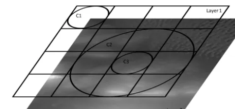
Figure 1.Diagram of the relationships among a Lebesgue measure, scale and geophysical variable.

rcos(2π x2) −2π rx1sin(2π x2) rsin(2π x2) 2π rx1cos(2π x2)

=2π r2x1. Therefore, s=RR

Ady1dy2= RR

A0|J (x1, x2)|dx1dx2=π r 2_s

0, which is equal to its area. However, s0 and s do not obey the one-dimensional rule because the Jacobian matrix is not diagonal.

Layer 1 in Fig. 1 shows the relationship between the Lebesgue measure and scale. The measure space =

[x:0≤xk≤4, k=1,2] is regularly divided by the unit squareA0. Let scales sC1=m2_C1(C1),sC2=m2_C2(C2)and sC3=m2_C3(C3) be the Lebesgue measures of disc ob-servation footprints C1, C2 and C3, respectively. Then, m2_C1(·)=m2_C2(·)=m2_C3(·) because they are the same Lebesgue measure functions. That is, if {Ai} is the set with the smallest volume that covers C1, then simi-lar sets {Ai+2} and {Ai×3+2} can be used (with the origin located in the upper-left corner) to cover C3 and C2 with the smallest volumes, respectively. Here, Ai+2=xi:xi,k+2, xi,k∈Ai, k=1,2 and Ai×

3+2=xi:xi,k×3+2, xi,k∈Ai, k=1,2, which proves that functions m2_C1(·), m2_C2(·) and m2_C3(·) collect the de-sired set based on the same scheme; therefore, they are identical. Additionally,sC2=m2_C2(C2)=P

I2(Ai×3+2) is much larger thansC1=m2_C1(C1)=PI2(Ai)andsC3= m2_C3(C3)=P

I2(Ai+2). Therefore, the scale of C2 is not equal to the two other scales because the volumes of their subsets are different. However, their scales are governed by one-dimensional rules because their measures are identical and the Jacobian matrices between them are diagonal. 3.2 Stochastic variables in data assimilation

Instead of using Eqs. (5) and (6), which are discrete in time, we use Ito process-formed expressions with the one-dimensional infinitesimals ds and dt to formulate a continuous-time (or continuous-scale) state and observation. A geophysical variable can be regarded as a real function V (s, t ), and it maps the space R2, L2, m2

related to an element of state vectorX at a specific scales and timet.

In Fig. 1, layer 2 presents a heterogeneous geophysical variable in the entire region. If we aggregate layer 2 into layer 1 and let each pixel intensity be the value for a geo-physical variable in that pixel, then the measure space  is heterogeneous. A geophysical variable represents a spa-tial average in a specific observation footprint with a specific scale. Therefore, the geophysical variables in C1 and C3 are not equal because their observation footprints are different, and the geophysical variables in C2 and C3 are also different because the scale changes. The former introduces that the geophysical variables vary with the location, and the latter states that the geophysical variables are scale dependent.

If the statistical properties of the geophysical variable are available, we can construct an explicit stochastic equation for it. We introduce the time-dependent Ito process Eq. (1) to define the geophysical variable process:

dV =p (t )dt+q (t )dW (t ) . (9) Similarly, the geophysical variable is supposed to evolve via a stochastic process, for which the dynamic process and un-certainty are allowed to vary with scale,

dV =ϕ (s)ds+σ (s)dW (s) , (10) where ϕ (s) and σ (s) are the scale-based drift rate and volatility rate, respectively. The geophysical variable is a probabilistic process with respect to scale and thus has scale-dependent errors, where the scale should shift forward or backward based on the condition that the scale follows the one-dimensional rule.

Equation (9) can be regarded as a continuous-time version of Eq. (5), i.e. the estimation of the state is equal to the in-tegral of Eq. (9) over a time interval. Here, p (t ) indicates the physical process with respect to time, andq (t )is the er-ror only caused by the evolution of time; thus, model erer-rorη in Eq. (5) contains more parts thanq (t ). Equation (10) im-plies that the value and variance of a geophysical variable may change if the scale changes. The formulation of ϕ (s) should consider the spatial heterogeneities and physical pro-cess variations among different scales, which together con-stitute the deterministic part of a geophysical variable. How-ever, neither of them is well understood in a general theoreti-cal study. Therefore,ϕ (s)is conceptualised in Eq. (10). Par-ticularly, if the study region is homogeneous, then the values of a variable that are observed at the same place are identical between the large scale and fine scale, andϕ (s)can be left out. Due to the integral over the space of Brownian motion, σ (s)is the stochastic part, meaning that scale transformation produces uncertainties.

The state in the forecasting step can be expressed by Eq. (9) because only time is involved. In the analysis step of data assimilation, the state does not pertain to time, and

we assume that the scale has a quantifiable effect on the er-rors in this step; thus, both the states and observations can be defined by Eq. (10).

3.3 Expression of scale transformation in a stochastic data assimilation framework

First, we provide the following lemma.

Lemma 1: for ∀s0>0, let W∗(0)=W (s0)− W (s0) , . . ., W∗(s)=W (s0+s)−W (s0); then,W∗(s) s≥0 is a Brownian motion.

Remark on Lemma 1: obviously, W∗

is Brownian motion because W∗(0)=0

and the increments W∗(si+1)−W∗(si) are equal to W (s0+si+1)−W (s0+si). Therefore, EW∗(si+1)−W∗(si)=0 and Var

W∗(si+1)−W∗(si)=si+1−si.

Note that in the definition of Brownian motion, the param-eter starts at zero. However, the scale is realistically greater than zero, which means that it cannot be directly applied in Brownian motion. Therefore, Lemma 1 is logical because it implies that W (s) s≥s0 is an equivalent expression of W∗(s) s≥0. Therefore, beginning with the standard scale, the Brownian motion and stochastic calculus with respect to scale can be further developed.

In the following content, we use Brownian motion with a parameter that starts ats0to define the scale-dependent geo-physical variables; therefore, the classic expressions above are changed. According to Lemma 1, Eq. (3) is given by

[I, I](s)=

s Z

s0

σ2(u)du. (11)

Additionally, the integral form of Eq. (10) is

V (s)=V0+ s Z

s0

ϕ (u)du+

s Z

s0

σ (u)dW (u) , (12)

whereV0=V (s0), and the drift of Eq. (12) is

V0+

s Z

s0

ϕ (u)du.

Similarly, Eq. (4) becomes

f (s, I (s))=f (s0, I (s0))+ s Z

s0

fu(u, I (u))du

+

s Z

s0

fI(u, I (u)) σ (u)dW (u)

+

s Z

s0

+1

2 s Z

s0

fI I(u, I (u)) σ2(u)du.

Now, we make the following assumptions.

Assumption 1: the scale transformations between the state and observation spaces of data assimilation obey the one-dimensional rule as defined in Sect. 3.1.

Assumption 2: in the forecasting step, the model unit equals the scale of the state space, and both of them are con-stant.

Assumption 3: in the analysis step, the state, observation and observation operator are scale dependent. Only one ob-servation is added into the data assimilation system at a time. In assumption 1, the one-dimensional rule ensures that scale changes in a sense of geometrical similarity (for exam-ple, from a larger square observation footprint to a smaller square observation footprint, or from C2 to C3 as pre-sented in Fig. 1). Therefore, based on assumption 1, scale only varies in one-dimensional space, meaning that the cor-responding scale transformation is an integral over one-dimensional space.

Assumption 2 indicates that the model unit and state scale are supposed to be the same and both invariant in space and time. Thus, there is no scale transformation in the forecasting step; thus, Eq. (9) can adequately describe this step.

Based on assumption 3, the analysis step is related to the scale. The scale transformation is only involved in the pro-cess of mapping the state vector from state space to observa-tion space. According to Eq. (10), the state and observaobserva-tion in the analysis step are

dX=ϕX(s)ds+σX(s)dW (s) (13) and

dY =ϕY(s)ds+σY(s)dW (s) , (14) whereϕX(s),σX(s),ϕY(s)andσY(s)represent the scale-dependent drift rates and volatility rates of stateXand obser-vationY, respectively.ϕ (s)also implies the heterogeneities and physical processes from standard scale to a specific scale, which may be hard to formulate.σ (u)can be regarded as the stochastic perturbation with respect to scale.

Based on the above discussion, the integral forms of the state are

X (sX)=X0+ sX

Z

s0

ϕX(s)ds+ sX

Z

s0

σX(s)dW (s) . (15)

For the observation, we have

Y (sY)=Y0+ sY

Z

s0

ϕY(s)ds+ sY

Z

s0

σY(s)dW (s) . (16)

In Eqs. (15) and (16), the timet is omitted, andsX,sY,X0 andY0represent the scale of the state space, scale of the ob-servation space, state ins0and observation ins0, respectively. These formulas prove that the value of state varies with the changes of scale.

The Bayesian equation of data assimilation (Eq. 7) pro-duces the posterior PDFp (X|Y )that is associated with the likelihood functionp (Y|X)and the distributions of the state and observation. In addition, under the condition that the variances exist, assumption 1 states that the scales vary in one-dimensional space, which results in

X∼N 

X0+ sX

Z

s0

ϕX(s)ds, sX

Z

s0

σ_X2(s)ds 

 and (17)

Y∼N 

Y0+ sY

Z

s0

ϕY(s)ds, sY

Z

s0

σ_Y2(s)ds 

. (18)

Equations (17) and (18) are the prior PDFs of state and ob-servation with respect to scale in state space and obob-servation space, respectively. These two prior PDFs are introduced into the Bayesian theorem that is reformulated by scale.

Then, we calculate the posterior PDF. The scale-dependent observation operator isH (s, I ), which suggests that the ob-servation operator and its parameters are both susceptible to the scale. IfH (s, I )is defined, its continuous partial deriva-tives areHs(s, I ),HI(s, I )andHI I(s, I ). In line with Ito’s Lemma, we get an estimation of observation in the obser-vation space (the notations(u, X (u))and(u)were omitted, Hs=Hs(u, X (u)),σX=σX(u), etc.)

H (sY, X (sY))

=H (s0, X0)+ sY

Z

s0

Hsdu+ sY

Z

s0

HIσXdW (u)

+

sY

Z

s0

HIϕXdu+ 1 2

sY

Z

s0

HI IσX2du

=H (s0, X0)+

sY

Z

s0

Hs+HIϕX+1

2HI Iσ 2 X

du

+

sY

Z

s0

HIσXdW (u) . (19)

Assumption 1 suggests that the observation and state spaces have the same probability measure; thus, the Brownian motions in these two spaces are equiva-lent. Equation (19) can also be rewritten by replacing s0 with sX, namely H (sY, X (sY))=H (sX, X (sX))+ RsY

sX

Hs+HIϕX+1

2HI IσX2

du+RsY

sXHIσXdW (u), and

then we obtain

− 

H (sX, X (sX))+ sY

Z

sX

Hs+HIϕX+ 1 2HI Iσ

2 X

du 



+

sY

Z

sX

(−HIσX)dW (u) . (20)

Equation (20) can be regarded as an Ito process, and its drift is

Y (sY)− 

H (sX, X (sX))+ sY Z

sX

Hs+HIϕX+

1 2HI Iσ

2 X

du



. (21)

The last integral term in Eq. (21) is the difference in the first-order differential observation operator between the state scale sX and the observation scalesY. This term illustrates that the mapping process should consider not only the obser-vation operator but also the first-order differential term when state is mapped to the observation space. The former is typ-ically determined from the literature, whereas the latter was derived in this study for the first time. This result prompted us to further consider the first-order differential of the obser-vation operator when calculating the representativeness error.

The quadratic variation of Eq. (20) is sY

Z

sX

H_I2σ_X2du. (22)

This equation suggests that the uncertainty in the observation error includes the change in the observation operator from scalesXtosY. Therefore, Eqs. (21) and (22) can be combined to produce

p (Y|X)=NY (sY)−hH (sX, X (sX))+

sY

Z

sX

Hs

+HIϕX+1

2HI Iσ 2 X

dui, sY

Z

sX

H_I2σ_X2du. (23)

Based on Eqs. (17), (18) and (23),p (Y|X),p (X)andp (Y ) are stochastic functions that depend on the scale; thus, the posterior PDF of the state is scale-dependent as well.

In particular, if Y is a direct observation, which means that the observation is of the same physical quantity and scale as the state, and for simplicity, assume that X is only influenced by scale-dependent Gaussian noises, viz. H (s, X (s))=X (s)=X0+

Rs

s0dW (s). Then the result be-comes

Y (sY)−X (sY)=Y (sY)−X (sX)− sY

Z

sX

dW (u) and (24)

p (Y|X)=N{Y (sY)−X (sX) ,|sY −sX|}. (25)

In Eq. (24), the integralRsY

sXdW (u)can be regarded as the

noise based on the increment of Brownian motion with re-spect to scale, and its expectation equals zero.

The significance of Eqs. (20)–(25) is that the effect of scale on the posterior PDF can be determined quantitatively. In ad-dition to the model error and instrument error (both were not introduced explicitly in this study because they have little in-fluence on the error caused by scale transformation), a new type of error in data assimilation was discovered in the analy-sis step. The expectation of the posterior PDF may vary with the scale of the state space ifY is an indirect observation, and the variance of the drift depends on the difference be-tweensY andsX(based on Eq. 22). In addition, ifY is a di-rect observation andXis only influenced by scale-dependent Gaussian noises (Eqs. 24 and 25), the expectation of the pos-terior PDF is the difference betweenY andX, and the vari-ance is equal to the increment of Brownian motion with re-spect to the scale. Additionally, if the results are not derived from assumption 1, i.e. the scale varies randomly, the poste-rior PDF is more complex because the Jacobian matrix in the Lebesgue integration of scale transformation is arbitrary. 3.4 Example: the stochastic radiative transfer

equation (SRTE)

To explicitly show how the stochastic scale transformations impact assimilation, we introduce an illustrative example based on the scales presented in Fig. 1. Assume that in the analysis step, the state has the standard scales0, whose ob-servation footprint is the unit squareA0. If the scale of ob-servation space issC1and its observation footprint is the disc C1, then the Jacobian matrix of the transformation between the scales of the state space and observation space is not diag-onal according to the statements in Sect. 3.1, leading the two scales to not obey the one-dimensional rule and be against assumption 1. However, if the scales of state space and ob-servation space aresC3 andsC2, respectively, assumption 1 is met, and it can be determined that sX=sC3=π₄s0 and sY =sC2=9π

4 s0.

Now the scales of state space and observation space obey the one-dimensional rule, and we further presume that the measure spacein Fig. 1 is free of spatial heterogeneities and dynamic process variations depending on scale. Conse-quently, the drift rateϕ (s)=0. If the value of state in the standard scale is denoted asX0and assuming thatσ (s)=1, then the prior PDF of state isX∼N X0,

π₄s0−s0

accord-ing to Eq. (17), whereπ₄s0−s0

is not a real number and is only used to indicate the variation when the scale changes.

If H (s, X (s))=X (s), the observation has the same physical quantity as the state, and ac-cording to Eq. (25), the likelihood function is p (Y|X)=N{Y (sY)−X (sX) ,|sY −sX|} = N{Y (sY)−X (sX) ,|sC2−sC3|} =

NnY (sY)−X (sX) ,

9π 4s0−

π 4s0

o

To formulate the likelihood function in the case that the observation is different from the state, the SRTE will be employed in the following text. The SRTE is a stochas-tic integral-differential equation that describes the radiative transfer phenomena through a stochastically mixed immisci-ble media. Scientists have developed analytical or numerical methods for finding the stochastic moments of the solution, such as the ensemble averaged and the variance of the ra-diation intensity (Pomraning, 1998; Shabanov et al., 2000; Kassianov and Veron, 2011).

Consider the general expression of the SRTE (leaving out the scattering and emission),

−µdI (τ )

dτ = −I (τ ) , (26)

whereI (τ ),µandτare the radiation intensity, coefficient of radiation direction and optical depth, respectively.

To tie into more substantial random optical properties of the transfer media, such as absorption and scattering, the op-tical depthτ is assumed to be stochastic. This suggests that the optical depth is a scale-dependent Ito process and can be expressed as

dτ (s)=ϕτ(s)ds+στ(s)dW (s) . (27) This causes the radiation intensity to depend on scale.

The analytical solution of Eq. (26) is I (τ )=I0eτ/µ, whereI0=I (τ (s0)).

SRTE can be considered as a concrete instance of a stochastic observation operator by defining H (s, x (s))=

I (x)=I0ex/µ. Therefore, its first- and second-order deriva-tives are Hs(s, x (s))=0, Hx(s, x (s))= 1

µI0ex/µ and Hxx(s, x (s))=_µ12I0e

x/µ_{. Based on Ito’s Lemma,}

dI (τ (s))=dH (s, τ (s))=Hs(s, τ (s))ds

+Hx(s, τ (s))dτ (s)+ 1

2Hxx(s, τ (s))dτ (s)dτ (s)

= 1

µI0e

τ (s)/µ_{dτ (s)+} 1 2µ2I0e

τ (s)/µ_{dτ (s)dτ (s)}

= 1

µI (τ (s))dτ (s)+

1

2µ2I (τ (s))dτ (s)dτ (s)

=

1

µI (τ (s))

στ(s)dW (s)+

1

µI (τ (s))

ϕτ(s)ds

+

1 2µ2I (τ (s))

σ2 τ(s)ds

=

_σ2 τ(s) 2µ2 +

ϕτ(s) µ

I (τ (s))ds+

_σ

τ(s) µ

I (τ (s))dW (s) .

(28)

The radiation intensity is a scale-dependent Ito process. The difference between Eq. (28) and the general Ito process is that there is a primitive functionI (τ (s))in the integral term. Therefore, the uncertainty of the radiation intensity is more complex because it is related to both the change of scale and the primitive function.

Integrating both sides of Eq. (28) yields the general solu-tion of the radiasolu-tion intensity,

I (τ (s))=C·exp

Z

σ_τ2(s) 2µ2 +

ϕτ(s) µ

ds

+ Z _σ

τ(s) µ dW (s) , (29)

where the constantC∈R. Equation (29) further indicates thatI (τ (s))is a scale-dependent Ito process.

Considering that the optical depthτ is the state, the radia-tion intensityIis the observation andI (τ (s))is the observa-tion operator, the results in Sect. 3.3 could easily be applied here. For example, Eqs. (20) and (23) become

Y (sY)−H (sY, X (sY))=I (τ (sY))−I (τ (sX))

− sY Z sX 1 µ2 _σ2 τ

2µ+ϕτ+ σ_τ2I (τ )

2µ2

I2(τ )du

−

sY

Z

sX

στ µ2I

2_{(τ )dW (u) , (30)}

p (Y|X)=N

I (τ (sY))−I (τ (sX))

−

sY

Z

sX

1 µ2I

2_{(τ ) σ}2

τ

2µ+ϕτ+ σ_τ2I (τ )

2µ2 du, sY Z sX

σ_τ2 µ4I

4_{(τ )du}

. (31)

Then, the posterior PDF of the data assimilation can be de-termined by Eqs. (27), (29) and (31).

4 Discussion and conclusions

4.1 Discussion

Our study offered a stochastic data assimilation framework to formulate the errors that are caused by scale transformations. The necessity of the methodology, the difference from pre-vious works by other investigators, and the advantages and limitations of this study are discussed as follows.

onto R. Correspondingly, as the integrals of random pro-cesses with respect to random propro-cesses, stochastic lus was ultimately adopted. Second, using stochastic calcu-lus can also formulate the errors caused by scale transfor-mations. The study proceeds with and improves the under-standing of representativeness error in terms of scale. The results did not only prove the conventional point that the un-certainties of these errors mainly depend on the differences between scales but also indicated that the first-order differ-ential of the non-linear observation operator should be incor-porated in representativeness error. Third, the error caused by scale transformation was presented in a general form. The drift and quadratic variation of error were formulated by Eqs. (21) and (22), respectively, and both defined the proba-bility distribution space ofp (Y|X). Last, stochastic calculus can be extended to meet a general scale transformation and formulate the corresponding representativeness error, which was unattainable in previous work. For example, if the scale changes randomly, say, from an irregular footprint to another irregular footprint, the stochastic equation can offer a multi-ple integral to present this type of scale transformation, such asV (x, y)=V0+

Y R

Y0 X R

X0

ϕ (x, y)dxdy+

Y R

Y0 X R

X0

σ (x, y)dW1(x) dW2(y), whereW1(x)andW2(y)are two independent Brow-nian motions.

The significant innovation of this work is as follows. We developed a more rigorous formulation of the scale and scale transformation based on Lebesgue measure, which places the related concepts in a rigorous mathematical framework and then provides a new understanding of the errors caused by scale transformation. In addition, due to the Ito process-formed state and observation, a stochastic data assimilation framework was proposed by considering the non-linear oper-ators, heterogeneity of a geophysical variable and a general Gaussian representativeness error. The scale transformation is also non-linear if the one-dimensional rule is not applied. Additionally, Ito process-formed state and observation offer the drift rate (i.e.ϕ (s)in Eq. 10) to formulate the heterogene-ity associated with scale transformation. It also permits the representativeness error to be general Gaussian in this frame-work. If all the integrands in Eqs. (13) and (14) are non-linear functions instead of constants, then these two equations can be integrated over the field of Brownian motion, and state and observation are the general Gaussian processes of scale. Based on these functions, the representativeness error is a general Gaussian process.

As a theoretical exploration towards scale transformation and stochastic data assimilation, there is still much room for improvement. First, we reduced the scale transformation by the one-dimensional rule, and let the variables in data assim-ilation evolve regularly according to assumptions 1–3; thus, only the ideal result was investigated. Therefore, an in-depth and comprehensive exploration should be conducted in the future to describe other situations in the real world.

How-ever, the use of either an arbitrary scale transformation or the geophysical variable without ignoring the drift rates will ob-tain lengthy results. Therefore, the second improvement fo-cuses on how to make the formulation more concise. Lastly, noting that all the results in our framework were given in terms of probability, it is necessary to implement real-world applications of these theoretical results, such as introducing some concrete dynamic models to formulate the Ito process-formed geophysical variable of scale.

4.2 Conclusions

In this study, we mainly addressed two basic problems as-sociated with scale transformation in Earth observation and simulation. First, we produced a mathematical formalism of scale and scale transformation by employing measure the-ory. Second, we demonstrated how scale transformation and its associated errors could be presented in a stochastic data assimilation framework.

We revealed that the scale is the Lebesgue measure with respect to the observation footprint or model unit. The scale is related to the shape and size of a footprint, and scale trans-formation depends on the spatial change between different footprints. We then defined the geophysical variable, which further considers the heterogeneities and physical processes. A geophysical variable consequently expresses the spatial average at a specific scale.

We formulated the expression of scale transformation and investigated the error structure that is caused by scale transformation in data assimilation using basic theorems of stochastic calculus. The formulations explicate that the first-order differential of the non-linear observation opera-tor should be considered in representativeness error, and the uncertainty of representativeness error is directly associated with the difference between scales. A concrete physical mod-els (SRTE) was introduced to demonstrate the results when observation operator is non-linear.

This work conducted a theoretical exploration of formu-lating the errors caused by scale transformation in a stochas-tic data assimilation framework. We hope that the stochasstochas-tic methodology can benefit the study of these errors.

Appendix A: Notation

Table A1.Basic notations.

 Non-empty space

F σ-algebra

µ Measure

dV Variable process

W (s) Brownian motion

(, F, µ) Measure space

In N-dimensional Lebesgue volume

mn Lebesgue measure or an outer measure onRn

Ln Lebesgueσ-algebra ofRn

R

fdmn Lebesgue integral |J (·)| Jacobian determinant

Table A2.New notations.

Notation Name Explanation Index

s Scale The observation footprint or model unit to observe or model a

geo-physical variable

Sects. 1 and 3.1

A0 Unit square inR2 Sect. 3.1

s0 Standard scale A Lebesgue integral whereA0is the unit area Sect. 3.1

One-dimensional rule Two scales are geometrically similar Eq. (8)

V Geophysical variable Estimation of a variable at a specific scale Sect. 3.2

dX State process Ito process-formed state Eq. (13)

dY Observation process Ito process-formed observation Eq. (14)

X0 State ats0 Eq. (15)

Y0 Observation ats0 Eq. (16)

sX Scale of state space Eq. (15)

Competing interests. The authors declare that they have no conflict of interest.

Acknowledgements. We thank the executive editor of NPG, Olivier Talagrand, and his kind help and valuable comments on our manuscript. We also thank Peter Jan van Leeuwen and another anonymous reviewer for their valuable comments and suggestions. This work was supported by the NSFC projects (grant numbers 91425303 and 91625103) and the CAS Interdisciplinary Innovation Team of the Chinese Academy of Sciences.

Edited by: Olivier Talagrand

Reviewed by: Peter Jan van Leeuwen and one anonymous referee

References

Apte, A., Hairer, M., Stuart, A. M., and Voss, J.: Sampling the poste-rior: An approach to non-Gaussian data assimilation, Physica D, 230, 50–64, https://doi.org/10.1016/j.physd.2006.06.009, 2007. Atkinson, P. M. and Tate, N. J.: Spatial scale problems and

geostatistical solutions: a review, Prof. Geogr., 52, 607–623, https://doi.org/10.1111/0033-0124.00250, 2000.

Bartle, R. G.: The Elements of Integration and Lebesgue Measure, Wiley, New York, 1995.

Billingsley, P.: Probability and Measure, 2nd Edn., John Wiley & Sons, New York, 1986.

Bocquet, M., Pires, C. A., and Wu, L.: Beyond Gaussian Statistical Modeling in Geophysical Data Assimilation, Mon. Weather Rev.,

138, 2997–3023, https://doi.org/10.1175/2010MWR3164.1,

2010.

Bocquet, M., Wu, L., and Chevallier, F.: Bayesian design of control space for optimal assimilation of observations. Part I: Consistent multiscale formalism, Q. J. Roy. Meteor. Soc., 137, 1340–1356, https://doi.org/10.1002/qj.837, 2011.

Crow, W. T., Berg, A. A., Cosh, M. H., Loew, A., Mohanty, B. P., Panciera, R., de Rosnay, P., Ryu, D., and Walker, J.: Upscaling sparse ground-based soil moisture observations for the validation of coarse-resolution satellite soil moisture products, Rev. Geo-phys., 50, 3881–3888, https://doi.org/10.1029/2011RG000372, 2012.

Eyink, G. L., Restrepo, J. M., and Alexander, F. J.: A mean field ap-proximation in data assimilation for nonlinear dynamics, Physica D, 195, 347–368, https://doi.org/10.1016/j.physd.2004.04.003, 2004.

Famiglietti, J. S., Ryu, D., Berg, A. A., Rodell, M., and Jackson, T. J.: Field observations of soil moisture vari-ability across scales, Water Resour. Res., 44, W01423, https://doi.org/10.1029/2006WR005804, 2008.

Giménez, D., Rawls, W. J., and Lauren, J. G.: Scaling properties of saturated hydraulic conductivity in soil, Geoderma, 27, 115–130, 1999.

Goodchild, M. F. and Proctor, J.: Scale in a digital geographic world, Geogr. Environ. Model., 1, 5–23, 1997.

Gruber, A., Dorigo, W. A., Zwieback, S., Xaver, A., and Wagner, W.: Characterizing coarse-scale representativeness of in situ soil moisture measurements from the

interna-tional soil moisture network, Vadose Zone J., 12, 522–525, https://doi.org/10.1002/jgrd.50673, 2013.

Hakuba, M. Z., Folini, D., Sanchez-Lorenzo, A., and Wild, M.: Spa-tial representativeness of ground-based solar radiation measure-ments, J. Geophys. Res.-Atmos., 118, 8585–8597, 2013.

Hodyss, D. and Nichols, N. K.: The error of

repre-sentation: Basic understanding, Tellus A, 66, 1–17,

https://doi.org/10.3402/tellusa.v67.24822, 2015.

Huang, G., Li, X., Huang, C., Liu, S., Ma, Y., and Chen, H.: Representativeness errors of point-scale ground-based solar radiation measurements in the validation of remote sensing products, Remote Sens. Environ., 181, 198–206, https://doi.org/10.1016/j.rse.2016.04.001, 2016.

Itô, K.: Stochastic integral, P. Jpn. Acad., 22, 519–524, 1944. Janji´c, T. and Cohn, S. E.: Treatment of Observation

Er-ror due to Unresolved Scales in Atmospheric Data

Assimilation, Mon. Weather Rev., 134, 2900–2915,

https://doi.org/10.1175/MWR3229.1, 2006.

Karatzas, I. and Shreve, S. E.: Brownian Motion and Stochastic Cal-culus, 2nd Edn., Springer-Verlag, New York, 1991.

Kassianov, E. and Veron, D.: Stochastic radiative transfer in Marko-vian mixtures: past, present, and future, J. Quant. Spectrosc. Ra., 112, 566–576, https://doi.org/10.1016/j.jqsrt.2010.06.011, 2011. Li, X.: Characterization, controlling, and reduction of uncertain-ties in the modeling and observation of land-surface systems, Sci. China Ser. D, 57, 80–87, https://doi.org/10.1007/s11430-013-4728-9, 2014.

Li, X. and Liu, F.: Can Point Measurements of Soil Moisture Be Used to Validate a Footprint-Scale Soil Moisture Product?, IEEE T. Geosci. Remote Sens., submitted, 2017.

Lin, H., Flühler, H., Otten, W., and Vogel, H. J.: Soil architec-ture and preferential flow across scales, J. Hydrol., 393, 1–2, https://doi.org/10.1016/j.jhydrol.2010.07.026, 2010.

Lorenc, A. C.: Atmospheric Data Assimilation, Meteorological Of-fice, Bracknell, 1995.

Lorenc, A. C.: Analysis methods for numerical weather prediction, Q. J. Roy. Meteor. Soc., 112, 1177–1194, 1986.

Merz, R., Parajka, J., and Blöschl, G.: Scale effects in concep-tual hydrological modelling, Water Resour. Res., 45, 627–643, https://doi.org/10.1029/2009WR007872, 2009.

Miller, R. N.: Topics in data assimilation:

stochastic processes, Physica D, 230, 17–26,

https://doi.org/10.1016/j.physd.2006.07.015, 2007.

Miller, R. N., Carter, E. F., and Blue, S. T.: Data assimila-tion into nonlinear stochastic models, Tellus A, 51, 167–194, https://doi.org/10.1034/j.1600-0870.1999.t01-2-00002.x, 1999. Miralles, D. G., Crow, W. T., and Cosh, M. H.: Estimating spatial

sampling errors in coarse-scale soil moisture estimates derived from point-scale observations, J. Hydrometeorol., 11, 1423– 1429, 2010.

Narsilio, G. A., Buzzi, O., Fityus, S., Yun, T. S., and Smith, D. W.: Upscaling of Navier–Stokes equations in porous media: Theoret-ical, numerical and experimental approach, Comput. Geotech., 36, 1200–1206, 2009.

Pomraning, G. C.: Radiative transfer and transport phenom-ena in stochastic media, Int. J. Eng. Sci., 36, 1595–1621, https://doi.org/10.1016/S0020-7225(98)00050-0, 1998. Ran, Y. H., Li, X., Sun, R., Kljun, N., Zhang, L., Wang, X. F., and

covariance carbon flux measurement for upscaling net ecosystem productivity to field scale, Agr. Forest Meteorol., 230–231, 114– 127, https://doi.org/10.1016/j.agrformet.2016.05.008, 2016. Ryu, D. and Famiglietti, J. S.: Multi-scale spatial correlation and

scaling behavior of surface soil moisture, Geophys. Res. Lett., 33, 153–172, 2006.

Shabanov, N. V., Knyazikhin, Y., Baret, F., and Myneni, R. B.: Stochastic modeling of radiation regime in discontinu-ous vegetation canopies, Remote Sens. Environ., 74, 125–144, https://doi.org/10.1016/S0034-4257(00)00128-0, 2000. Shreve, S. E.: Stochastic Calculus for Finance II, Springer-Verlag,

New York, 2005.

Talagrand, O.: Assimilation of observations, an introduction, J. Me-teorol. Soc. Jpn., 75, 191–209, 1997.

van Leeuwen, P. J.: Representation errors and retrievals in linear and nonlinear data assimilation, Q. J. Roy. Meteor. Soc., 141, 1612– 1623, https://doi.org/10.1002/qj.2464, 2014.

van Leeuwen, P. J.: Nonlinear data assimilation for high-dimensional systems, in: Frontiers in Applied Dynamical Sys-tems: Reviews and Tutorials, Vol. 2, Springer-Verlag, New York, 2015.

Vereecken, H., Kasteel, R., Vanderborght, J., and Harter, T.: Upscaling hydraulic properties and soil water flow processes in heterogeneous soils: a review, Vadose Zone J., 6, 1–28, https://doi.org/10.2136/vzj2006.0055, 2007.