www.nonlin-processes-geophys.net/22/205/2015/ doi:10.5194/npg-22-205-2015
© Author(s) 2015. CC Attribution 3.0 License.
Improved variational methods in statistical data assimilation
J. Ye1, N. Kadakia1, P. J. Rozdeba1, H. D. I. Abarbanel1,2, and J. C. Quinn3
1Department of Physics, University of California, San Diego, La Jolla, CA 92093-0374, USA 2Marine Physical Laboratory (Scripps Institution of Oceanography), University of California, San Diego, La Jolla, CA 92093-0374, USA
3Intellisis Corporation, 10350 Science Center Drive, Suite 140, San Diego, CA 92121, USA
Correspondence to: H. D. I. Abarbanel ([email protected])
Received: 18 August 2014 – Published in Nonlin. Processes Geophys. Discuss.: 10 October 2014 Revised: 3 March 2015 – Accepted: 23 March 2015 – Published: 7 April 2015
Abstract. Data assimilation transfers information from an observed system to a physically based model sys-tem with state variables x(t ). The observations are typ-ically noisy, the model has errors, and the initial state
x(t0) is uncertain: the data assimilation is statistical. One can ask about expected values of functions hG(X)i on the path X= {x(t0), . . .,x(tm)} of the model state through the observation window tn= {t0, . . ., tm}. The conditional (on the measurements) probability distribution P (X)=
exp[−A0(X)]determines these expected values. Variational methods using saddle points of the “action”A0(X), known as 4DVar (Talagrand and Courtier, 1987; Evensen, 2009), are utilized for estimating hG(X)i. In a path integral formula-tion of statistical data assimilaformula-tion, we consider variaformula-tional approximations in a realization of the action where measure-ment errors and model errors are Gaussian. We (a) discuss an annealing method for locating the pathX0giving a consis-tent minimum of the actionA0(X0), (b) consider the explicit role of the number of measurements at eachtnin determining A0(X0), and (c) identify a parameter regime for the scale of model errors, which allowsX0to give a precise estimate of
hG(X0)iwith computable, small higher-order corrections.
1 Introduction
In a broad spectrum of scientific fields, transferring the in-formation contained in L observed data time series yl(tn); l=1, . . . , L; n=0, . . . , mto a physically based model of the processes producing those observations allows the esti-mation of unknown parameters and unobserved states of the model within an observation window{t0, . . ., tm}. As a
sam-ple of these fields, we note applications in meteorology (Tala-grand and Courtier, 1987; Evensen, 2009; Lorenc and Payne, 2007), geochemistry (Eibern and Schmidt, 1999), fluid dy-namics (Zadeh, 2008) and plasma physics (Mechhoud et al. , 2013), among many others.
The conditional probability distribution P (X)=exp[−A0(X)] allows evaluation of expected values of physically interesting functions G(X) along the path. P (X) is conditioned on the measurements yl(tn); l=1, . . . ,L;n=0, . . . ,m. These areL-dimensional, while the model state isD-dimensional; it is usually the case that DL. Data assimilation seeks to use the information in
y(tn) to estimate unknown parameters in the model and unobserved states of the model. If this is accomplished, one uses prediction fort > tmto examine the validity of the model.
The actionA0(X)contains terms giving a measurement’s influence on P (X), terms propagating the model between the measurement timestn, and a term−log[P (x(0))] repre-senting the uncertainty in the initial state (Abarbanel, 2013). We discuss the familiar case where additive measurement er-rors are independent at each tn and Gaussian with covari-ance Rm−1(l,l0, t); l, l0=1, . . . , L. The model is a physi-cal differential equation, discretized in space and time and satisfying theD-dimensional stochastic discrete time map xa(n+1)=fa(x(n))+R
−1/2
f (a,b)ηb(n); a, b=1, . . . , D with iid Gaussian noise errorηa(n)∼N(0, 1). We takeRm(l, l0,n)=Rm(n) δl,l0andRf(a,b)=Rfδa,b.Rm(n)is zero
With these conditions, the action takes a familiar form:
A0(X)=
m
X
n=0 Rm(n)
2 L
X
l=1
xl(n)−yl(n)
2 +Rf 2 m−1 X n=0 D X a=1
xa(n+1)−fa(x(n)) 2
−log[P (x(0))]. (1)
The conditional expected value hG(X)i of a function G(X)on the pathX= {x(t0), . . .,x(tm)}is given as
hG(X)i =
R
dXG(X)exp [−A0(X)]
R
dXexp [−A0(X)] . (2)
One interesting functionG(X)isXitself, whose expected value gives us the average path over the measurement win-dow [t0,tm]. Estimates of the parameters andP (x(tm)) per-mit prediction fort > tm; in this window, one compares ob-servations and predictions using model output with a user-selected metric. No information is passed to the model in the prediction window. Importantly, good estimation of observed state variables (a “good fit”) is not sufficient to produce confi-dence in the quality of the model; good prediction is critical. To approximate the integralhG(X)i, we follow the station-ary path method of Laplace (Laplace, 1774) and seek saddle points in path space Xq labeled byq=0, 1 . . . satisfying ∂A0(X)/∂Xα=0. The index αis a label for the state and time α= {a, n}. To determine their importance in evaluat-ing the integral, Eq. (2) paths are sorted by increasevaluat-ing action levelsA0(Xq):A0(X0)≤A0(X1)≤ · · ·.
2 EvaluatinghG(X)i
We take the the usual data assimilation technique (Talagrand and Courtier, 1987; Evensen, 2009; Lorenc and Payne, 2007) several steps further by
1. showing how to find a consistent pathX0for the mini-mum action level using an annealing method,
2. demonstrating the importance of the number of mea-surementsLat each observation timetn, and
3. explaining how to make systematic perturbation correc-tions to hG(X0)i, i.e., G(X0) evaluated on the mini-mum action level path.
For nonlinear problems of interest, there may be many pathsXq;q=0, 1, . . . satisfying the saddle point condition. To assess their contributions tohG(X)i, we expandA0(X) in the neighborhood of eachXqas (note that all variables are notated in Table 2)
A0(X)=A0 Xq
+ X−Xqα
1γ
2 α1α2 X
q
X−Xqα
2
+X
r=3
A(r)(Xq) α1...αr
r! X−X q
α1. . . X−X q
αr. (3)
There is an implied sum over all paired Greek indicesαj. A sum over all terms with comparable action levelA0(Xq)then gives an approximation tohG(X)i.
Changing variables toUα=γαβ(Xq) (X−Xq)β leads to a contribution to the numerator ofhG(X)i in Eq. (2) from eachXq
exp−
A0(Xq) detγ (Xq)
Z
dU exp−U2−V Xq
G Xq+W Xq (4) where
V Xq=X
r=3
A(r)(Xq)α1...αr r!
γ Xq−1
U α1
. . .γ Xq−1
U αr
,
and
W Xq=X
k=1
G(k)(Xq) α1...αk
k!
γ Xq−1U α1
. . .γ Xq−1
U αk
.
The contributions to the denominator of Eq. (2) are identi-cal to Eq. (4), with the factor [G(Xq)+W (Xq)]replaced by unity. We sum over the contribution of eachXq to evaluate
hG(X)i.
If the lowest action levelA0(X0)is much smaller than all others, then exp[−A0(X0)] exp[−A0(Xq6=0)]and its con-tribution tohG(X)itotally dominates the integral. We have then that
hG(X)i =
R
dU exp −U2−V X0 G X0
+W X0 R
dU exp −U2−V X0 , (5)
plus exponentially small corrections from the action levels associated with other saddle pathsXq6=0.
3 Annealing to find a consistent minimum action level
A0(X0)
We now turn to an annealing method to find the path
X0 where exp[−A0(X0)] exp[−A0(Xq6=0)]. Within this method, we first examine the importance of the numberLof measurements at each observation timetn. We then present an argument that, in the integral Eq. (4), contributions to
us withhG(X)i ≈G(X0)with corrections that are a power series in Rf−1. The implication is that all statistical data as-similation questions, asRf/Rmbecomes large, can be well approximated by the contribution of the path X0 with the lowest action level A0(X0)along with corrections one can evaluate via standard perturbation theory. Variations about
hG(X0)iwould be small and computable.
The term in the action expressing uncertainty in the ini-tial model state x(0), P (x(0)), is often written assum-ing Gaussian variation about some base state xbase, so
−log[P (x(0)] ∝(x(0)−xbase)2Rbase/2, and this has the form of the measurement term evaluated atn=0. We incor-porate this expression into the term with coefficientRmin the action and no longer display it. This term, often called a prior, is also seen at the initial condition for the time evolution of the conditional probability distributionP (X).
3.1 Annealing details
The annealing method starts with the observation (Quinn, 2010) that the equation for the saddle points Xq simplifies at Rf =0. The action atRf=0 has no information about the model, and relies solely on the measurements. The saddle point solution isxl(n)=yl(n);l=1, 2, . . . ,Lfor all observa-tion times. The other (D−L) components of the model state vector are undetermined, and the solution is quite degenerate. As we increaseRf, the action levels split, and, depending on Rm,Rf,Land the precise form of the dynamical vector field
f(x), there will be 1, 2, . . . saddle points ofA0(X). The sad-dle points of interest are local minima.
For anyRf>0, the search for saddle points of the action requires an unconstrained numerical optimization problem to be solved: minimizeA0(X). This is 4DVar in its “weak” formulation (Talagrand and Courtier, 1987; Evensen, 2009). The methods we have utilized for performing this numerical optimization range from Newton and quasi-Newton methods (Press et al., 2012) to more sophisticated interior point meth-ods (Waëchter , 2002). Each search for saddle paths requires an initial guessX(0)that is then iterated via the algorithm to produceX(1), thenX(2), and continuing on to produce a final pathX(final)for each value ofRf.
We begin the annealing process by choosing the initialRf, denotedRf0, as very small, but nonzero; indeed, ifRf0was chosen to be vanishing, the set of optimal paths would be all paths whose measured components match the data, and whose unmeasured components are entirely unconstrained. Such a solution is infinitely degenerate and gives no more insight than the data themselves. Therefore, we begin the search at someRf01 with the firstL(m+1) components of X(0) taken as the observations y(tn); n=0, 1, . . . , m. The remaining components of X(0) are chosen from a uni-form distribution reflecting the dynamical range of the un-measured state variables.
Because the search algorithm is an iterative process with potentially many basins of attraction, it is not evident which
minimum or saddle point we will hit in this initial optimiza-tion. Accordingly, we actually start withNI copies of this procedure, makingNI independent, with initial choices of
X(0;r); r=1, 2, . . . , NI at Rf0; in other words, we initi-ate many such annealing procedures in parallel. TheseNI choices differ in the unmeasured components of the path, independently drawn from a uniform distribution over the range of each variable.
In the next step of the annealing process, the value of Rf is increased to Rf0ξ whereξ >1. Using as our initial paths the final paths X(final;r) from the previous optimiza-tion with Rf=Rf0, we perform the numerical optimiza-tion procedure once again, independently for each of theNI paths. This results in a new set ofNI saddle pathsX(final;r); r=1, 2, . . . ,NIatRf =Rf0ξ.
This process is repeated as many times as desired, increas-ingRf from one iteration to the next by a power ofξ. We use theNI final paths from each value ofRf as the initial paths for the next value ofRf. The output is a set ofNI paths and action values for each value ofβ=0, 1, . . . ,βmax, and the action level for each of theNIfinal paths is plotted for each Rf. Specific examples of this will be presented below.
All of these optimizations, for each r and each β, is a 4DVar calculation for which we have used various algorithms (Press et al., 2012; Waëchter , 2002). In a sense, we can think of this as an ensemble version of 4DVar, with the important aspect that we performNI calculations of 4DVar at eachβ.
AsRf/Rm grows large, the errors in the model dimin-ish relative to the measurement errors and impose high-precisionx(n+1)≈f(x(n))on the model dynamics. The noise in the measurement has been taken to be GaussianN(0, σ2), so the measurement error term in the action satisfies aχ2distribution (NIST Handbook of Statistical Methods , 2012) with meanRmσ2(m+1)L/2 and standard deviation Rmσ2
√
(m+1)L/2. We note that this observation has been made by Bennett (2002) when the weak form of 4DVar, here using the action as the objective function, results in accurate representation of the dynamics.
Using properties of theχ2distribution, the action level for largeRf approximately approaches a lowest value
A0
X0→ Rmσ
2
2 L(m+1)
1±√ 1
(m+1)L/2
. (6)
σ2is the noise level inyl(n)and (m+1) is the number of measurement times tn. This provides a consistency condi-tion on the identificacondi-tion of the path X0 by giving a con-sistent minimum action value A0(X0). If the action levels revealed by our annealing procedure do not give this result forA0(X0), it is a sign that the data are inconsistent with the model.
the action level on the next saddle pathA0(X0)A0(X1), all expected valueshG(X)iare given byG(X0), and correc-tions due to fluctuacorrec-tions about that path. The contribution to the expected values of the path integral forhG(X)ifromX1
with the next action level is exponentially smaller, of order exp[−(A0(X1)−A0(X0))].
The annealing procedure discussed above is different from standard simulated annealing (Aguiar e Oliviera et al., 2012). We call this annealing because varyingRf is similar to vary-ing a temperature in a statistical physics problem whereRf is inversely proportional to the temperature. At high tempera-tures, smallRf, the dynamics among the degrees of freedom xa(n)is essentially irrelevant, and we have a universal solu-tion where the observed degrees of freedom match the obser-vations. As the temperature is decreased, the dynamics plays a more and more significant role, and allowed paths “freeze” out. Action levels play the role of energy levels in statistical physics, and as the action is positive definite, the paths are directly analogous to instantons in the Euclidian field theory represented byA0(X)(Zinn-Justin, 2002).
The calculations used in the annealing process may seem formidable. We have chosen NI=100 in the examples we present now, because we wish to make clear the scope of the calculations and their implications. We chose this rather than concentrating now on optimizing the algorithms. This will come with some experience with different model structures. Nonetheless, due to the manner in which the action levels space themselves and split Rf is increased, it might prove less demanding to use a largeNI for the first few values of Rf, and then significantly decrease the number of paths from NI. Our goal is to trace accurately just the lowest action value stateX0and the nextX1to estimate the scale of the domi-nance ofA0(X0)in performing the path integral.
4 Examples from the Lorenz96 model
We now present the results of a set of calculations on the Lorenz96 (Lorenz, 2006) model used frequently in geophys-ical data assimilation discussions as a test bed for proposed methods. The model hasDdegrees of freedomxa(t ) satisfy-ing the differential equation
˙
xa(t )=xa−1(t ) (xa+1(t )−xa−2(t ))−xa(t )+f+ζa(t ); (7)
a=1, . . . , D; x−1(t )=xD−1(t ), x0(t )=xD(t ), xD+1(t )=x1(t ); ζa(t ) is N(0, Rf−1) Gaussian noise. f =8.17, for which the xa(t ) are chaotic (Kostuk, 2012). We studiedD=20 and addedf as an additional degree of freedom satisfying f˙=0. The number of model equations in the action is therefore equal toD+1.
We performed a twin experiment in which we solved these equations, withζa(t )=0 and with an arbitrary choice of initial conditions x(0) using a fourth-order Runge–Kutta solver with1t=0.025 over 160 steps in time. Here,t0=0 and tm=T =4. We then added iid Gaussian noise with
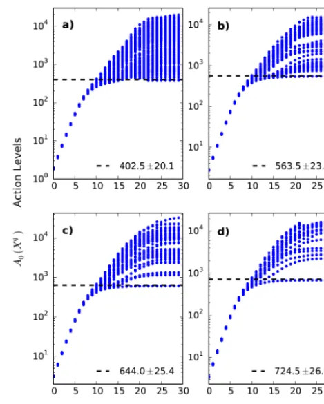
Figure 1. Action levels as a function ofRf for the Lorenz96 model,
D=20, Rf0=0.01. (a) At L=5, we used y1(t ), y3(t ), y5(t ), y7(t ), andy9(t )in the action; (b) atL=7,y11(t )andy13(t )are
added; (c) atL=8,y15(t ) is added; and (d) atL=9, y17(t )is
added. The expected values of the lowest action level are denoted by black dashed lines.
zero mean and variance σ2=0.25 to each time series. L=1, 2, . . . of the data series were then represented in the action at each measurement timetnduring our annealing pro-cedure. In our calculations,Rf0=0.01 andξ=2.
In the action, we selectedRm=4, the inverse variance of the noise added to the data in our twin experiment, so the minimum action level we expect is 80.5L±8.97
√
L. The paths are (m+1) (D+1)=3381-dimensional. Our search for minimum paths used a BFGS routine (Press et al., 2012) to which we provided an analytical form of the gradient of A0(X). The search was initialized withNI=100 times with initial paths from a uniform distribution of values in the in-terval [−10, 10].
We also investigated using the IPOPT public domain nu-merical optimization package (Waëchter , 2002) and found that it also worked well, giving essentially the same results as BFGS. Any existing method for 4DVar should work as well for this annealing procedure.
0
2
4
6
8
10
12
−10
−5
0
5
10
15
x3
(t
)
; o
bse
rve
d
a)
x3(t)data x3(t)est x3(t)pred0
2
4
6
8
10
12
Time (arb. units)
−10
−5
0
5
10
15
x12
; u
no
bse
rve
d
b)
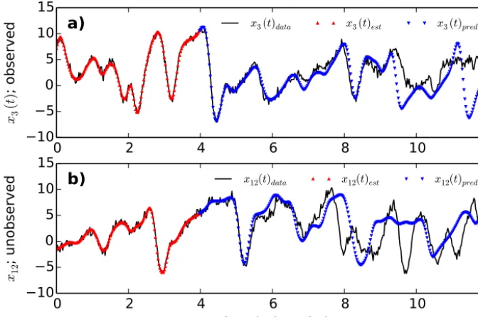
x12(t)data x12(t)est x12(t)predFigure 2. Data, estimated, and predicted time series for the Lorenz96 model (Lorenz, 2006) withD=20,L=8. (a)x3(t )was an observed
state variable, and (b)x12(t )was unobserved. The data (black), the estimated state variable (red), and the predicted state variable (blue) are
shown for each of them.
paths of the action Eq. (1); as L increases, the lowest ac-tion level visibly separates from the others. At the bottom of each panel, we indicate the lowest action level value and its standard deviation. The next-lowest action levelA0(X1), for L=5, 7, 8, and 9, is at 403.8, 749.8, 1161.6, and 2256.1, re-spectively. This means that forL=5 we would have to sum over the contributions of many pathsXq to evaluate the ex-pected valuehG(X)i. AtL=7 or higher,X0dominates the integral. Our estimate for the forcing parameter, set to 8.17, was 8.22 at largeβ.
We think it important to note that if we had begun our search for the saddle point pathsXq at large values ofRf, we would be almost sure to miss the actual pathX0, which gives the lowest action level, since the Hessian matrix ofA0 is ill conditioned when Rf is large; see Fig. 4.6 in Quinn (2010).
Another sense of why beginning a search at large values of Rf may fail to find the action level identified in the annealing approach is that the basin of attraction of the minimum ac-tion level is likely to be so small, relative to the size of path space, that “falling into it” through an arbitrary initial path used in any version of a variational procedure is unlikely. The annealing method systematically tracks the known minimum for very smallRf and, in that manner, starts in and remains in the appropriate basin of attraction.
The real test of an estimation procedure in data assimi-lation is not accuracy in the estimation of measured states and fixed parameters, but accuracy in prediction beyond the observation window. The predictions require accurate esti-mation of the unobserved model state variables at the end of
the observation window. Indeed, one can achieve good “fits” of observed variables that lead to inaccurate predictions for t > tm=T (Abarbanel, 2013).
As this is a twin experiment, we show in Fig. 2 the data, the estimated state variable, and the predicted state variable for an observed variablex3(t )and for an unobserved variable x12(t ) for L=8. In a real experiment, we could not com-pare our estimates for the parameters or the unobserved state variables. Although the estimation procedure for the pathX0
with the minimum action value is rather good, both in esti-mating the 12 unobserved states and the one parameter, there nevertheless exist errors in our knowledge of the full state (x(t )=4). The predictions thus lose their accuracy in time because of the chaotic nature of the trajectories atf=8.17.
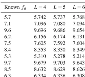
In the Lorenz96 equations, one usually has a single forc-ing parameter f. To see how well our procedure works for several unknown parameters, we introduced ten dif-ferent forcing parameters fa into the Lorenz96 model at D=10: x˙a(t )=xa−1(t ) (xa+1(t )−xa−2(t ))−xa(t )+fa, that is, with no fluctuations in the dynamics. Noise was added to the solutions to the Lorenz96 system before thexa(t )are used as data. ForD=10, the lowest action level stands out from the rest atL=4. In Table 1, we show our estimates for the ten forcing parameters forL=4, 5, and 6, as well as the actual value used in the calculations of the data. In these es-timates, and for the single forcing parameter reported above forD=20, there is a known source of bias (Kostuk et al., 2012). As one can see in the examples, it is small here.
Table 1. Known and estimated forcing parameters for the Lorenz96 model atD=10, andL=4, 5, and 6.
Knownfa L=4 L=5 L=6
5.7 5.742 5.737 5.768
7.1 7.096 7.080 7.094
9.6 9.696 9.686 9.654
6.2 6.156 6.174 6.131
7.5 7.605 7.592 7.604
8.4 8.353 8.330 8.349
5.3 5.310 5.278 5.214
9.7 9.679 9.703 9.643
8.5 8.632 8.629 8.626
6.3 6.334 6.336 6.308
give some sense of what one might expect if the model were totally wrong, in the sense that the data we presented came ei-ther from a completely different model system or from enor-mously noisy data, we presented data from a collection of 1963 Lorenz model (Lorenz, 1963) oscillators to a Lorenz96 D=10 model. Twelve time series data are generated by four individual Lorenz63 (Lorenz, 1963) systems with different initial conditions. Gaussian white noise with zero mean and standard deviationσ=0.5 are added to each time series. All these “data”yl(t )are rescaled to lie within [−10, 10].
We then place these signals as “data” in the action with the model taken as Lorenz96D=10; the single forcing pa-rameter is treated as a time-dependent state variable obey-ingf˙=0. We useL=5 andL=6 as measurements using the data time series taken in the order y1(t ), y3(t ), y5(t ), y7(t ),y9(t )for L=5, andy1(t ),y3(t ),y5(t ),y7(t ),y9(t ), y2(t )forL=6. In Fig. 3 we display the action levels versus log[Rf/Rf0] =β associated with this forL=5 andL=6. Results for other values ofLare consistent with these. This example provides a graphic illustration of the inconsistency of the data and the model and how this makes its appearance in the annealing procedure.
We also investigated, but do not display here, the action levels when the parameterfis held at a different value in the model than was used for generating the data. In particular, we generated the data withf=8.17 and then heldf=18 in evaluating the action levels for a Lorenz96 model withD=5 andL=1 and 2. In each case, no minimum action level split from the collection ofXq and no level was close to the con-sistent χ2condition discussed above. This actually empha-sizes the importance of allowing the variational method to include all parameters as state variables with a zero vector field, allowing the estimation of the parameters along with the unmeasured state variables.
We now have seen that a consistent smallest action level can be identified via an annealing process, and the depen-dence of the action levels on the number of measurements, L, has been demonstrated. We have no formal proof that the pathX0gives a global minimum of the action; our criteria of
0 5 10 15 20 25 30 100
101 102 103 104 105
a)
0 5 10 15 20 25 30 104
105 106 107
b)
β (Rf=Rf02β)
A0
(X
q)
A
ct
io
n
Le
ve
ls
Figure 3. Action levels as a function ofRf for the Lorenz96 model,
D=10,Rf0=0.01. (a)L=5 and (b)L=6 when the wrong data
are used for the Lorenz96 model. We actually used data from four realizations of the Lorenz63 model (Lorenz, 1963). The structure of the action levels versusRf shows no trace of the minimum
al-lowed level Eq. (6). This indicates that the data and the model are incompatible. The action levels are also quite large, and, forL=6, numerous and not well separated.
consistency with Eq. (6) and excellent predictions after the observation window are functionally useful features of the procedure.
5 Corrections to the contribution of a saddle path to hG(X)i
We turn back to the evaluation of the path integral forhG(X)i
in Eq. (2). In that integral for our action, we have 1
2A (2) 0 (X)=γ
2
αβ(X)=Rm(n)δa,lδb,l0+Rfhαβ(X)
andA(r)0 (X)=Rfg(r−2)(X),
forr≥3. The functionsh(X)andg(X)are derivable from the form ofA0(X). These are to be evaluated atX=Xq for theqth saddle path.
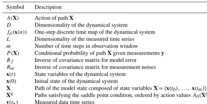
Table 2. List of important mathematical notations (in alphabetical order).
Symbol Description
A(X) Action of path X
D Dimensionality of the dynamical system
fa(x(n)) One-step discrete time map of the dynamical system
L Dimensionality of the measured time series
m Number of time steps in observation window
P (X) Conditional probability of path X given measurements y
Rf Inverse of covariance matrix for model error Rm Inverse of covariance matrix for measurement noises x(t ) State variables of the dynamical system
x(0) Initial state of the dynamical system
X Path of the model state composed of state variables X= {x(t0), . . .,x(tm)}
Xq Paths satisfying the saddle point condition, ordered by action valuesA0(Xq)
y(tn) Measured data time series
6 Conclusions
We have examined the path integral formulation of data assimilation Eq. (2) and asked how well a variational ap-proach to the conditional expected values of functionsG(X) on the pathX= {x(0),x(1),x(2), . . .,x(m)}can approxi-mate the integral. We use Laplace’s method, which estiapproxi-mates the path integral by seeking saddle paths of the action where ∂A0(X)/∂Xα=0. This approximation is widely used in me-teorology and other fields, where it is known as weak 4DVar (Talagrand and Courtier, 1987; Evensen, 2009; Lorenc and Payne, 2007). The action is the cost function that is mini-mized.
When measurement errors and model errors are distributed as iid Gaussian noise, we have described an annealing method in the strengthRf with which the model errors enter the action that permits the following of a collection of ac-tion levels fromRf =0, where the saddle paths are known precisely, through a set of increasing values of Rf at each of which a numerical optimization algorithm produces a set of saddle paths that are used as the initial conditions for the solution of the variational approximation at the next larger value of Rf. This permits the identification of a lowest ac-tion level associated with a saddle path X0 whereA0(X0) is split from the action values for the other possible saddle pathsXq>0) at eachRf:A0(X0) < A0(Xq>0)). The contri-bution ofX0then dominates the integral.
We also explored the dependence of the action levels re-vealed through the annealing method on the number of mea-surementsLmade at each observation time. WhenLreaches and exceeds a critical value, related to the number of unsta-ble directions in the deterministic chaotic dynamics of the model, the contribution of the pathX0is either certainly the dominant contribution to the conditional expected value of G(X), or it is the only path satisfying the saddle path con-dition. By expanding the integrand of Eq. (2) about X0we
argued that the resulting corrections to the contribution of
X0produced a power series inRf−1.
In previous work with variational principles for data as-similation, we are unaware of any procedure such as our an-nealing method usingRf to identify a consistent minimum action. Nor are we aware of a systematic exploration of the dependence of the action levels on the number of measure-ments at each observation time. (Of course, there is the dis-cussion in Quinn, 2010, which suggested this work.) Finally, we do not know of any previous discussion of the corrections to the variational approximation, which here is shown to con-sist of small perturbations when the resolution of the model error term in the action is increased; namely,Rf becomes large.
The relation of the annealing method to familiar 4DVar calculations (Talagrand and Courtier, 1987; Evensen, 2009) is simple to state: each set of calculations during the anneal-ing inRf, at each value ofRf, is a 4DVar calculation. The annealing has the added advantage of allowing one to estab-lish an identified lowest action value pathX0that gives the dominant contribution to the quantities of interest, namely, the conditional expected values of functionsG(X) on the path.
stan-dard ensemble methods such as the ensemble Kalman filter (EnKF) (Evensen, 2009). However, that is a subject for an-other investigation of the annealing approach; we have fo-cused here only on variational methods.
We have worked within a framework where the measure-ment errors and the model errors in the data assimilation are Gaussian, with the inverse covariance of the model er-rors taken to be of orderRf. We have shown that the path that gives a consistent minimum action level can be traced by an annealing procedure starting with a setting where the dynamical model essentially plays no role,Rf ≈0, then sys-tematically increasing the influence of the model dynamics. As the scale of the model error reaches about 100 times the scale of the measurement error, the pathX0associated with a consistent global minimum action level dominates the path integral with corrections of order 1/Rf. The important role of the number of measurementsLat each measurement time is also demonstrated.
If the noise terms represented by the model errors are not Gaussian, one can still use the annealing method to identify a path with the lowest action level, but showing that perturba-tion theory about the pathX0giving that lowest action level is a power series inR−1f may not succeed. The precise way Rf enters the matrixγαα20(X0)determines that.
In this paper, we do not address the typical situation where the number of measurements actually available is less than that needed to allow the ground level of the actionA0(X0)to lie well below the next level. For a solution to that problem, we have used information from the waveform of the mea-surements as shown in some detail in Rey et al. (2014).
The results here justify the use of the variational approxi-mation in data assimilation, focus on the role of the number of measurements one requires for accuracy in that approxi-mation, and permit the evaluation of systematic corrections to the approximation when the form of the action is Eq. (1). We anticipate that our use of Gaussian model error and mea-surement error is a convenience and that other distributions of these errors will permit many of the same set of statements about the value of variational approximations to statistical data assimilation.
Acknowledgements. Partial support has come from the ONR
MURI program (N00014-13-1-0205). We are very appreciative of the considered comments of the anonymous referees during the discussion period of this paper. Indeed, one of the first referee’s questions led to the idea that the annealing approach could be useful in Monte Carlo estimations of the expected value path integrals.
Edited by: Z. Toth;
Reviewed by: two anonymous referees
References
Abarbanel, H. D.: Predicting the Future: Completing Models of Ob-served Complex Systems, Springer, New York, 2013.
Aguiar e Oliviera, H., Ingber, L., Petraglia, A., Petraglia, M. R., and Machado, M. A. S.: Stochastic Global Optimization and Its Applications with Fuzzy Adaptive Simulated Annealing, Vol. 35, Springer, New York, 2012.
Bennett, A. F.: Inverse Modeling of the Ocean and Atmosphere, Cambridge University Press, 2002.
Eibern, H. and Schmidt, H.: A four-dimensional variational chem-istry data assimilation scheme for Eulerian chemchem-istry transport modeling, J. Geophys. Res.-Atmos., 104, 18583–18598, 1999. Evensen, G.: Data Assimilation: The Ensemble Kalman Filter,
Springer, New York, 2009.
Kostuk, M.: Synchronization and statistical methods for the data assimilation of HVc neuron models, PhD thesis in Physics, Uni-versity of California, San Diego, available at: http://escholarship. org/uc/item/2fh4d086 (last access: 2 October 2014), 2012. Kostuk, M., Toth, B., Meliza, C., Margoliash, D., and
Abar-banel, H.: Dynamical estimation of neuron and network prop-erties II: path integral Monte Carlo methods, Biol. Cybern., 106, 155–167, 2012.
Laplace, P. S.: Memoir on the probability of causes of events, Mé-moires de Mathématique et de Physique, Tome Sixième, 1774. Lorenc, A. C. and Payne, T.: 4D-Var and the butterfly effect:
statisti-cal four-dimensional data assimilation for a wide range of sstatisti-cales, Q. J. Roy. Meteorol. Soc., 133, 607–614, 2007.
Lorenz, E. N.: Deterministic nonperiodic flow, J. Atmos. Sci., 20, 130–141, 1963.
Lorenz, E. N.: Predictability – a problem partly solved, in: Pre-dictability of Weather and Climate, edited by: Palmer, T. and Hagedorn, R., Cambridge University Press, 40–58, 2006. Mechhoud, S., Witrant, E., Dugard, L., and Moreau, D.: Combined
distributed parameters and source estimation in tokamak plasma heat transport, in: 2013 European Control Conference (ECC), 17–19 July, Zurich, 47–52, 2013.
NIST/SEMATECH e-Handbook of Statistical Methods:
http://www.itl.nist.gov/div898/handbook/ (last access: 12 Jan-uary 2014), 2012.
Press, W. H., Teokulsky, S. A., Vetterling, W. T., and Flannery, B. P.: Numerical Recipes in C: the Art of Scientific Computing, Cam-bridge University Press, 2012.
Quinn, J. C.: A path integral approach to data assimilation in stochastic nonlinear systems, PhD thesis in Physics, University of California, San Diego, available at: http://escholarship.org/uc/ item/0bm253qk (last access: 2 October 2014), 2010.
Rey, D., Eldridge, M., Kostuk, M., Abarbanel, H. D., Schumann-Bischoff, J., and Parlitz, U.: Accurate state and parameter estima-tion in nonlinear systems with sparse observaestima-tions, Phys. Lett. A, 378, 869–873, 2014.
Talagrand, O. and Courtier, P.: Variational Assimilation of Meteoro-logical Observations With the Adjoint Vorticity Equation, I: The-ory, Q. J. Roy. Meteorol. Soc., 113, 1311–1328, 1987.
Zadeh, K. S.: Parameter estimation in flow through partially sat-urated porous materials, J. Comput. Phys., 227, 10243–10262, 2008.