www.the-cryosphere.net/10/1161/2016/ doi:10.5194/tc-10-1161-2016
© Author(s) 2016. CC Attribution 3.0 License.
Characterizing Arctic sea ice topography using high-resolution
IceBridge data
Alek A. Petty1,2, Michel C. Tsamados3, Nathan T. Kurtz2, Sinead L. Farrell1,2,4, Thomas Newman1,4, Jeremy P. Harbeck2, Daniel L. Feltham5, and Jackie A. Richter-Menge6
1Earth System Science Interdisciplinary Center, University of Maryland, College Park, Maryland, USA 2Cryospheric Sciences Laboratory, NASA Goddard Space Flight Center, Greenbelt, Maryland, USA
3Centre for Polar Observation and Modelling, Department of Earth Sciences, University College London, London, UK 4NOAA Center for Weather and Climate Prediction, College Park, Maryland, USA
5Centre for Polar Observation and Modelling, Department of Meteorology, University of Reading, Reading, UK 6Cold Regions Research and Engineering Laboratory, Hanover, New Hampshire, USA
Correspondence to:Alek A. Petty ([email protected])
Received: 31 October 2015 – Published in The Cryosphere Discuss.: 24 November 2015 Revised: 2 May 2016 – Accepted: 17 May 2016 – Published: 31 May 2016
Abstract.We present an analysis of Arctic sea ice topogra-phy using high-resolution, three-dimensional surface eleva-tion data from the Airborne Topographic Mapper, flown as part of NASA’s Operation IceBridge mission. Surface fea-tures in the sea ice cover are detected using a newly devel-oped surface feature picking algorithm. We derive informa-tion regarding the height, volume and geometry of surface features from 2009 to 2014 within the Beaufort/Chukchi and Central Arctic regions. The results are delineated by ice type to estimate the topographic variability across first-year and multi-year ice regimes.
The results demonstrate that Arctic sea ice topography ex-hibits significant spatial variability, mainly driven by the in-creased surface feature height and volume (per unit area) of the multi-year ice that dominates the Central Arctic re-gion. The multi-year ice topography exhibits greater interan-nual variability compared to the first-year ice regimes, which dominates the total ice topography variability across both regions. The ice topography also shows a clear coastal de-pendency, with the feature height and volume increasing as a function of proximity to the nearest coastline, especially north of Greenland and the Canadian Archipelago. A strong correlation between ice topography and ice thickness (from the IceBridge sea ice product) is found, using a square-root relationship. The results allude to the importance of ice de-formation variability in the total sea ice mass balance, and provide crucial information regarding the tail of the ice
thick-ness distribution across the western Arctic. Future research priorities associated with this new data set are presented and discussed, especially in relation to calculations of atmo-spheric form drag.
1 Introduction
Figure 1. (a)Aerial photograph of the sea ice surface, taken off the coast of Barrow, Alaska.(b)Schematic of a sea ice floe (not to scale) featuring two large pressure ridges, one smaller pressure ridge and a sastruga (snow feature).
while snow redistribution features also distort the ice surface, caused by erosion (sastrugi) and deposition (dunes) (Thomas and Dieckmann, 2009). Snow drift features can build up alongside sails (snow banks), smoothing their slope and ex-tending their areal coverage. Visual imagery of the sea ice surface and a schematic of a typical FYI floe are given in Fig. 1.
In regions where the sail and keel density is high, the resultant obstructions to fluid flow (form drag) are thought to dominate the total drag on the ice cover over frictional (skin drag) effects (Arya, 1973; Leonardi et al., 2003; Tsama-dos et al., 2014). Ice deformation also impacts the internal strength of the ice pack, further altering the momentum trans-fer between the atmosphere and ocean (Martin et al., 2014). The sea ice strength is critical for understanding the resultant loads experienced by ice-breaking ships and offshore struc-tures (e.g. Timco and Weeks, 2010). Dynamical ice redistri-bution also contributes directly to the total thickness of Arc-tic sea ice (e.g. Thorndike et al., 1975), although this con-tribution to ice growth (over thermodynamics) has yet to be reliably quantified. In the Arctic, first-order estimates sug-gest that deformed ice could contribute up to ∼50 % of the total sea ice volume (Wadhams, 2000). The ice topography impacts sea ice melt variability through melt pond formation (e.g. Perovich and Polashenski, 2012), where the flatter (vari-able) topography of FYI (MYI) promotes shallow but exten-sive (deeper but less extenexten-sive) melt ponds to form on the sea ice surface (e.g. Polashenski et al., 2012). Increased un-derstanding of the sea ice topography is also of interest to the satellite (e.g. ICESat and CryoSat-2) and airborne (e.g. Ice-Bridge) altimeter communities, as the interpretation of radar returns over pressure ridges remains challenging (e.g. New-man et al., 2014).
Studies investigating sea ice morphology in detail (i.e. those resolving distinct pressure ridges at the metre scale) have been based predominantly on airborne and underwa-ter measurements (e.g. Tucker et al., 1979; Wadhams, 1980, 1981; Tucker et al., 1984; Wadhams and Davy, 1986; Haas, 2004; Martin, 2007; Rabenstein et al., 2010). More recently, Doble et al. (2011) used coincident autonomous underwater
vehicle (AUV) sonar and airborne laser profiling to perform a high-resolution, three-dimensional analysis of sea ice mor-phology; however this was limited to one region within the Beaufort Sea. Efforts have been made to compile existing data sets of pressure ridge morphology (Strub-Klein and Su-dom, 2012) and airborne surface profiling (Castellani et al., 2014), to increase spatial and temporal coverage. Unfortu-nately, these data remain sparse (they do not provide annual data on a basin scale), and are predominantly based on linear profiling of surface features.
In this study, we utilize recent, high-resolution data from the Airborne Topographic Mapper (ATM) laser altimeter, flown as part of NASA’s Operation IceBridge (OIB) mission (Krabill, 2013), to provide detailed information regarding the sea ice topography over a variety of Arctic sea ice regimes. IceBridge surveys conducted from Fairbanks, Alaska, ac-quire data over the predominantly FYI cover of the Beaufort and Chukchi seas, while surveys conducted from Thule and Kangerlussuaq, Greenland, sample the thicker, MYI pack of the Central Arctic, north of Greenland and the Canadian Archipelago. IceBridge offers a vast improvement over pre-vious data sets used to investigate ice topography, due to the combination of high spatial coverage and the use of a coni-cal scanner, which allows profiling of the ice surface in three dimensions. The continuous years of data collection (since 2009) also increasingly provide the potential to assess inter-annual variability within these two regimes.
The paper is organized as follows: Sect. 2 describes the data used in this study; Sect. 3 discusses the surface feature detection methodology; Sect. 4 presents and discusses the Arctic sea ice topography results; and conclusions are given in Sect. 5.
2 Data
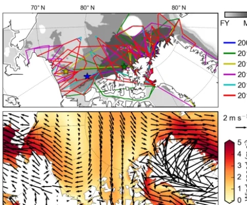
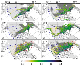
Figure 2.Top: IceBridge sea ice flight lines and estimated ice type over the western Arctic. The dark grey (light grey) background in-dicates regions where more than 80 % of the daily data within all IceBridge sea ice campaign dates (across all years) are estimated as MYI (FYI), while the medium grey indicates a mix of FYI and MYI, taken from the EUMETSAT OSI-SAF ice type mask. The coloured stars indicate locations of the various case studies, as highlighted in the relevant figures. Bottom: mean winds from January to March (2009–2014) taken from the ERA-I reanalyses.
OIB aircraft carry a suite of instruments designed to measure both land and sea ice, including their overlying snow cover. In this study, we primarily make use of data obtained by the Airborne Topographic Mapper (ATM) which is a conically scanning laser altimeter operating at 532 nm (Krabill et al., 2002). The ATM laser range and aircraft position/orientation are used to assign three-dimensional geographic coordinates to the point where each laser pulse reflects from the surface. The laser elevation data are referenced to the WGS-84 ellip-soid.
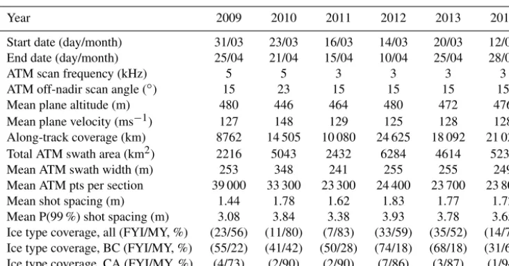
The across-track ATM swath width is determined by the maximum off-nadir scan angle, which is normally fixed at 15◦, giving a swath width of∼250 m, assuming a nominal flight altitude of∼460 m. Note that the scan angle was in-creased to 23◦in 2010, increasing the swath width. Various statistics regarding the IceBridge sea ice flights and ATM data are shown in Table 1. Each elevation measurement has a footprint of∼1 m and a vertical accuracy of 10 cm or bet-ter (Krabill, 2013). Martin et al. (2012) showed that for the IceBridge missions specifically, the ATM has an estimated horizontal accuracy of 74 cm, a vertical accuracy of 6.6 cm and a vertical precision of 3 cm. The high vertical resolution of the ATM makes it well suited to the detection of ridges with a characteristic sail height (upper surface extension of the ridge) of around 1–2 m (e.g. Wadhams, 2000). The shot-to-shot ATM spacing is variable (due to the conical scan) and depends on the location of the shot within the swath,
includ-ing a negligible shot spacinclud-ing at the edge of the swath, and a variable shot spacing of several metres around the centre of the swath (Krabill, 2013). The shot spacing at the centre of the swath is determined by the off-nadir scan angle, scan frequency and the plane’s altitude, pitch, roll and velocity.
The ATM surface elevation data are routinely used in the retrieval of sea ice freeboard, in conjunction with an auto-mated sea ice lead detection algorithm (Onana et al., 2013) based on coincident optical imagery of the surface from the Digital Mapping System (DMS) (Dominguez, 2010) as de-scribed in more detail by Kurtz et al. (2013). The DMS pro-vides geolocated, panchromatic or natural colour imagery that features an image resolution (pixel size) of∼10 cm, as-suming a nominal flight altitude of∼460 m, and covers the entire width of the ATM scan. An Applanix POS/AV preci-sion orientation system is used to geolocate and orthorectify the images (Brooks et al., 2012). Sea ice thickness is esti-mated from the sea ice freeboard using snow depth derived from the on-board snow radar system (Kurtz et al., 2013). The sea ice freeboard, thickness and snow depth product, at a 40 m spatial resolution that includes associated uncertainties, is available through the National Snow and Ice Data Cen-tre (NSIDC) (IDCSI4, Kurtz et al., 2015). Since 2012, Ice-Bridge has also provided the community with a quick-look data product, several months in advance of the standard prod-uct release (Kurtz et al., 2013). The IDCSI4 (2009–2013) and quick-look (2014–2015) 40 m spatially averaged sea ice data sets are used in the surface feature–ice thickness regression analysis (Sect. 4.3). However, in this study, we mainly utilize the raw∼1 m horizontal resolution ATM elevation data to characterize the surface profile within the entire ATM swath. We primarily analyse the ATM data from 2009 to 2014 in this study, but also make use of the recently released 2015 data in the surface feature–ice thickness regression analy-sis (Sect. 4.3). The IceBridge sea ice data coverage over the western Arctic from 2009 to 2014 is shown in Fig. 2.
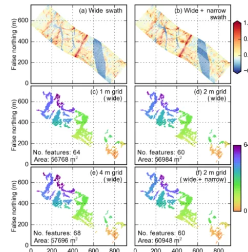
Since 2011, OIB has also operated a “narrow scan” ATM that features a lower across-track swath width of∼45 m, in-creasing the shot density in the centre of the swath (Krabill, 2014). These narrow scan ATM data will be combined with the regular (“wide scan”) ATM data in specific case studies to assess the potential uncertainties in the surface feature detec-tion from the lower mean spatial sampling of the wide scan ATM.
Visual validation of the surface feature detection scheme is carried out using the DMS imagery, while the POS/AV data are used for accurate geolocation of along-track positioning to determine bounds of evenly spaced ATM sections, as dis-cussed later.
Table 1.IceBridge ATM flight information. Note that all calculated quantities (rows 3–13) are based on the permissible sea ice sections, as described in Sect. 3. The ice type classification is also described in more detail in Sect. 3 (rows 11–13).
Year 2009 2010 2011 2012 2013 2014
Start date (day/month) 31/03 23/03 16/03 14/03 20/03 12/03 End date (day/month) 25/04 21/04 15/04 10/04 25/04 28/04
ATM scan frequency (kHz) 5 5 3 3 3 3
ATM off-nadir scan angle (◦) 15 23 15 15 15 15
Mean plane altitude (m) 480 446 464 480 472 476
Mean plane velocity (ms−1) 127 148 129 125 128 128 Along-track coverage (km) 8762 14 505 10 080 24 625 18 092 21 028 Total ATM swath area (km2) 2216 5043 2432 6284 4614 5232
Mean ATM swath width (m) 253 348 241 255 255 249
Mean ATM pts per section 39 000 33 300 23 300 24 400 23 700 23 800 Mean shot spacing (m) 1.44 1.78 1.62 1.83 1.77 1.72 Mean P(99 %) shot spacing (m) 3.08 3.84 3.38 3.93 3.78 3.65 Ice type coverage, all (FYI/MY, %) (23/56) (11/80) (7/83) (33/59) (35/52) (14/79) Ice type coverage, BC (FYI/MY, %) (55/22) (41/42) (50/28) (74/18) (68/18) (31/61) Ice type coverage, CA (FYI/MY, %) (4/73) (2/90) (2/90) (7/86) (3/87) (1/94)
of passive microwave and scatterometry data over the en-tire Arctic Ocean. We also utilize a data set quantifying the distance to the nearest coastline (http://oceancolor.gsfc.nasa. gov/DOCS/DistFromCoast/) to understand sea ice topogra-phy/deformation as a function of coastline proximity.
Finally, we use the National Snow and Ice Data Center (NSIDC) regional mask of the Arctic Ocean and surround-ing regions (http://nsidc.org/data/polar_stereo/tools_masks) (i) to ensure data are over sea ice, and (ii) to exclude regions (e.g. the Canadian Archipelago) from some of our analyses.
3 Sea ice topography characterization
There has been considerable discussion in the literature re-garding pressure ridges and how they should be defined (e.g. Hibler et al., 1974; Wadhams, 1981; Wadhams and Davy, 1986; Martin, 2007). In this study we employ the elevation threshold approach, which has been used extensively in pre-vious studies (e.g. Wadhams, 1980; Dierking, 1995; Martin, 2007; Tan et al., 2012; Castellani et al., 2014). Typically, a ridge (or surface feature) is detected if it has a height above the local level ice/snow surface greater than a chosen eleva-tion threshold. Different elevaeleva-tion thresholds are then used to differentiate different topographic features of the ice cover. Castellani et al. (2014), for example, used 20 and 80 cm thresholds to differentiate “big” sails from “small” sails/snow features. Sastrugi heights were measured during the Sever airborne program (Warren et al., 1999, Fig. 16b). A maxi-mum sastrugi height of 46 cm (north of Greenland) was sug-gested based on quadratic fits to in situ observations, mean-ing elevation thresholds higher than this are likely to exclude purely snow drift features. Results based on the lower eleva-tion threshold mean one can not talk solely of deformaeleva-tion features, due to the likely inclusion of snow features.
Alter-natively, higher elevation thresholds could result in the exclu-sion of a significant fraction of the ice topography variability. The choice of cut-off height can provide a significant impact on the sail/feature height distributions (e.g. Tan et al., 2012) and should be considered when analysing the surface feature data derived in this study.
In this study, we choose to focus on a lower elevation threshold of 20 cm, but also provide summary results and discussion of the analysis using a higher 80 cm threshold. Our results are therefore more representative of the total ice and snow topography variability, which is an important fac-tor when considering the potential impact of these results on estimates of atmospheric form drag over sea ice, an expected utility of this data set in the near future. For simplicity, we refer to all measured topographic snow or ice features in this analysis as “features”, instead of ridges or sails. Hibler et al. (1972) discussed the concept of a ridge link as the ele-mentary linear segments composing otherwise complex two-dimensional deformation features. In fact, our feature detec-tion algorithm (described in the following subsecdetec-tions) se-lects connected areas around a local maximum in each struc-ture, and our individual features can therefore be thought of as intermediate quantities between an elementary ridge link and the full ridge structure. Visual inspection across several case studies (not shown) demonstrates that for the higher el-evation threshold (80 cm), a linear approximation is more valid than for the features detected using a lower (20 cm) threshold. This idea will be explored further in Sect. 4.4.
likely to pick the peaks of the entire surface feature, as op-posed to linear profiling studies, which detect the peak of the surface feature along a random (linear) profile. In re-gions where surface features are sparse, the two-dimensional ATM scan makes it much more likely that we will detect a surface feature (higher than the chosen elevation threshold). These differences in approach, and the impact on the resul-tant sail heights especially, are discussed in more detail by Lensu (2003). The feature height distributions in this study are thus likely to differ from those presented previously (e.g. Wadhams, 1980). A recent study by Beckers et al. (2015) explored the difference in surface roughness (standard devi-ation of relative surface elevdevi-ation) statistics from linear and scanning airborne laser altimetry, for regions north of Sval-bard and in the Fram Strait. They found convergence of sur-face roughness statistics for sampling distances over several kilometres, especially for the drifting ice sampled north of Svalbard. Unfortunately their surface roughness data are dif-ferent to the surface feature data presented in this study. Fu-ture work will attempt to understand, in more detail, the po-tential differences between the surface feature distributions presented here, and the surface feature distributions gener-ated by linear profiling.
3.1 Feature-picking methodology
The following sections detail the surface feature detection scheme that is visually demonstrated in the case study given in Fig. 3. Further case studies are given in the supplemen-tary information, covering a range of ice types (Figs. S1–S3 in the Supplement). Note that these case studies are based on all individual ATM points within the bounds of the DMS image (∼350 m along-track in Fig. 3) for visualization pur-poses. In the processing of all ATM data (all results pre-sented in Sect. 4), the size of each ATM section processed is increased to 1 km along-track. This was a balance between having enough data to reliably estimate a level ice surface (discussed in the next subsection), and a small enough re-gion not be influenced by changes in the sea surface height. The Rossby radius, which indicates the length scale of ocean eddies, is&10 km for typical polar latitudes (Chelton et al., 1998), an order of magnitude greater than the 1 km section length chosen.
3.1.1 Level ice surface calculation
To detect features on the ice surface, we first define a level ice surface. Previous approaches include detecting regions where the ice elevation change is less than some threshold over some along-track distance (e.g. Wadhams and Horne, 1980), or detecting the modal ice surface within a given re-gion (e.g. Williams et al., 2015). In this study, we take a simi-lar approach to the recent, three-dimensional Antarctic study of Williams et al. (2015) and detect the most level ice surface within the relevant section. We calculate the cumulative
el-Figure 3.Example of the surface feature detection algorithm over-laid on a DMS image taken on the 23rd March 2011 as highlighted by the yellow star in Fig. 2.(a)DMS image;(b)raw ATM data overlaid on the DMS image;(c)elevation distribution for all ATM points within the section shown, where the blue line indicates the bounds of the calculated level ice surface and the red line indicates the feature height threshold;(d)gridded (2 m) ATM elevation rel-ative to the level ice surface;(e)unique surface features (>20 cm) and their elevation relative to the level ice surface;(f)unique surface feature identifier (features larger than 100 m2).
evation distribution of all ATM points within a 1 km section and find the percentile bin (using a bin width of 20 %) with the smallest elevation increase. This is equivalent to finding the modal elevation across percentile bins. The level ice sur-face calculation is demonstrated in Fig. 3c (and other case studies in the supplementary information). In Fig. 3c, the lowest elevation change is found at 15–35 %, meaning the level ice elevation was taken at the 25th percentile of the el-evation distribution, corresponding to a level ice elel-evation of
3.1.2 Data interpolation
All the raw, irregularly spaced ATM elevation data (within each 1 km section) are then projected on to a regu-larly spaced horizontal grid based on the EPSG:3413 po-lar stereographic projection (https://nsidc.org/data/icebridge/ projections_grids.html), using a linear interpolation scheme. The level ice elevation is subtracted to convert the data to a regularly spaced grid of elevation relative to the level ice surface (Fig. 3d). We note that, due to the on-ice scan pat-tern of the ATM, grid cell values are informed by a variable number of raw measurements, wherein the effects of spatial sampling and instrument noise will vary across the gridded elevations. Specifically, the higher shot spacing in the mid-dle of the ATM swath poses a potential for over-interpolation, depending on the horizontal grid resolution chosen. To inves-tigate this in more detail, the shot spacing was analysed for several flights across all OIB years, as summarized in Table 1 and demonstrated in the supplementary information (Fig. S5 in the Supplement). We analysed the near-maximum (99th percentile) spacing in each section, as the maximum spacing is often influenced by isolated ATM points caused by adja-cent data drop-out. The mean shot spacing is also shown in Table 1. This demonstrates that across all years (2009–2014), most of the data (99 %) have a shot spacing<4 m, meaning a horizontal grid resolution of 2 m was chosen (over half the near-maximum spacing). Problems can also occur in inter-polation around the ATM swath edge within the convex hull (the maximum region bounded by the corners of the ATM section), especially when the plane deviates from a linear trajectory (sections are not analysed if the pitch and/or roll is greater than a set threshold as discussed in Sect. 3.1.4). A kd tree algorithm (Maneewongvatana and Mount, 1999) is therefore used to detect the proximity of the projected ATM data to the raw ATM data. If the nearest raw ATM data point is further than a set distance away (5 m), then that data point is discarded.
3.1.3 Identifying unique surface features
All the gridded ATM elevation data below the chosen fea-ture height threshold (20 cm) are then masked. We scan the masked/gridded ATM data for connected data points using a 3×3 structuring element that considers data points to be con-nected if they touch adjacently or diagonally. Features which occupy an area less than a set threshold (100 m2) are dis-carded. The information is still retained in the “bulk” ice to-pography statistics (area fraction/volume of surface features), as discussed later.
Further segmentation is carried out to increase the geomet-rical characterization of the surface features. We search each of the connected components for local maxima, and a water-shed filter (Soille and Ansoult, 1990) is used to find the shal-lowest contour that separates each local maxima. These local maxima must be separated from each other (horizontally) by
Figure 4.Example feature detection algorithm for a 1 km ATM sec-tion in 2011. The top row shows the raw ATM data from both the regular wide scan(a)and from the combined wide and narrow scan (b). Panels(c–e)show the features detected using a 1 m(c), 2 m (d)and 4 m(e)gridding of the regular wide scan ATM data, while (f)shows the results from the 2 m gridding of the combined wide and narrow scan ATM data. Panels(c–e)also show the number of surface features (>20 cm) detected and the total area of these fea-tures.
at least 10 m, as in previous studies (e.g. Martin, 2007). This segmentation is highlighted by the large feature in Fig. 3 that has been split into several segments, each dominated by a local maxima. This step is especially crucial when using a relatively low elevation threshold (e.g. 20 cm as in most of this study) as large features often merge together around their lower elevation bases.
results. Note that Fig. 4 demonstrates the feature detection scheme over a typical 1 km section.
3.1.4 Individual feature and bulk topography statistics Before proceeding with the ATM processing, the POS/AV data are used to assess the pitch, roll and altitude of the plane within the relevant 1 km ATM section. If the mean pitch or roll is greater than 5◦or the mean altitude of the plane is out-side the range 300–700 m (based on the nominal sea ice flight altitude of∼460 m), then the ATM section is not processed. The number of ATM points within the 1 km section is also calculated as low-lying cloud; leads and ATM malfunction can result in significant regions of ATM drop-out. The mean number of ATM points within a 1 km ATM section (sum-marized in Table 1) varies from∼40 000 points in 2009 to
∼20 000 points from 2011 onwards, when the ATM scan an-gle and frequency were reduced. We therefore use a thresh-old of 15 000 ATM points (75 % of the minimum) to ensure reasonable data coverage within each ATM section analysed. We calculate the surface feature height (hf) by finding the height of all points within each unique surface feature relative to the level ice surface, and define hf as the peak (maximum) value. We calculate the surface feature area (Af), which is equal to the number of grid points within each fea-ture multiplied by the square of the grid resolution chosen (2 m). We compute the centre of mass of each feature (rc), which we use as the feature position. Note that we do not weight the surface feature heights based on their areal cover-age (Af).
While not being a major focus of this study, we also com-pute the covariance matrix (analogous to an inertia matrix) of each feature as
C= Z
Af
(ri−rc)×(ri−rc)d2ri, (1)
where ri is the position of each point within the unique feature, and the integration is performed over the full fea-ture area. Cs and Cp are the small (secondary) and large (primary) eigenvalues of Crespectively, meaning the ratio
R=(Cp/ Cs)1/2 gives the degree of elongation of the fea-ture (the ratio of long over short axis, assuming an elliptical shape). We present this analysis to highlight further poten-tial applications of this unique data set, and to demonstrate the impact of the elevation threshold on the geometry of the features detected in this study (Sect. 4.4).
Several additional bulk properties of the ice topography are calculated directly within the feature detection scheme. For all (1 km) ATM sections, we collect the (i) mean x/y
section location, (ii) ATM swath area coverage (used to es-timate ice area, assuming minimal open water), (iii) number of features detected, (iv) feature area coverage (all, includ-ing small features<100 m2), (v) feature area coverage (only large features >100 m2), (vi) mean surface feature height
(all, including small features) and (vii) mean surface feature height (only large features). The volume of surface features per unit ice area,Vf, is calculated by multiplying the appro-priate mean feature height (with or without small features included) by the total feature area coverage within the sec-tion, and dividing by the total swath area (units of m). Note that here we use the mean height of all the points included within each feature to calculate the mean feature height and volume (within each section), whereas in the individual fea-ture height analysis, we take the maximum (peak) height of the feature. Using the maximum feature height has the ben-efit of being independent of the elevation threshold (if the same feature is detected across different thresholds) and the size of the feature detected. The surface feature height,hf, is thought to be more relevant to form drag calculations (dis-cussed in Sect. 4.4). The surface feature volume (per unit area),Vf, is an integrator of the size (height and areal cov-erage) and density of the surface features, and is more of an indicator of the total ice topography variability.
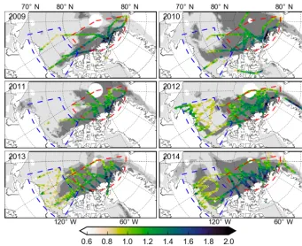
Figure 5.Surface feature height,hf, from 2009 to 2014, detected using a 20 cm elevation threshold. The dark grey (light grey) background indicates regions where more than 80 % of the daily data within each year’s IceBridge sea ice campaign dates are estimated as MYI (FYI), while the medium grey indicates a mix of FYI and MYI. The red (blue) dashed lines represent the Central Arctic (Beaufort/Chukchi) regions used in this study. The data are plotted using hexagonal bins.
4 Results and discussion
4.1 Ice topography characterization 4.1.1 Feature height variability
Figure 5 shows maps of the surface feature height (hf) from 2009 to 2014, detected using an elevation threshold of 20 cm. The results demonstrate predominantly higher surface fea-tures (&1 m) in the CA region, mainly north of Greenland and the Canadian Archipelago, and predominantly lower fea-tures (.1 m) in the BC region. Feature heights are markedly higher (&1.5–1.7 m) along the northern coast of Greenland and, in 2012, along the eastern coast of Greenland, within the Fram Strait. The feature height also increases towards the Beaufort Sea coastline in 2012 (increasing up to ∼1.2 m), which coincides with a tongue of MYI that same year.
Figure 6 shows the probability distributions of surface fea-ture heights within the CA and BC regions for all feafea-tures, and for the features estimated as either FYI or MYI, using the OSI-SAF ice type mask (discussed in Sect. 3). We also ex-clude data within the Canadian Archipelago and Fram Strait (using the NSIDC Arctic Ocean mask) from this analysis. Statistics from these distributions are summarized in Table 2. Note that a bin width of 10 cm is used in these probability
distributions, although the mean and standard deviation are calculated independently. Before interpreting these distribu-tions, it is worth noting that the spatial sampling in 2009 is lower than all other years (Table 1) and is weighted more to-wards the thick ice directly north of Greenland (Fig. 5). The sampling in the BC region in 2011 is also noticeably sparse. The spatial sampling increases markedly in 2012–2014, al-lowing for a more reliable discussion of interannual variabil-ity within both regions.
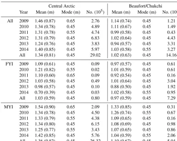
Table 2.Surface feature height statistics (mean and mode) taken from the probability distributions shown in Fig. 6. The value in the brackets (next to the means) equals 1 standard deviation of the relevant distribution. The third column (under each region) shows the number of surface features detected.
Central Arctic Beaufort/Chukchi
Year Mean (m) Mode (m) No. (105) Mean (m) Mode (m) No. (105) All 2009 1.46 (0.87) 0.65 2.76 1.14 (0.74) 0.45 1.21
2010 1.34 (0.78) 0.45 4.89 1.11 (0.67) 0.45 1.49 2011 1.31 (0.78) 0.55 4.74 0.99 (0.58) 0.45 0.43 2012 1.31 (0.79) 0.45 6.83 1.02 (0.64) 0.45 4.43 2013 1.24 (0.76) 0.45 3.83 0.94 (0.57) 0.45 3.31 2014 1.40 (0.85) 0.45 5.97 1.03 (0.58) 0.55 3.27 All 1.34 (0.81) 0.45 29.02 1.02 (0.63) 0.45 14.16
FYI 2009 1.09 (0.61) 0.45 0.09 0.97 (0.57) 0.45 0.61 2010 1.21 (0.82) 0.55 0.02 1.01 (0.59) 0.45 0.61 2011 1.10 (0.60) 0.65 0.09 0.92 (0.54) 0.45 0.16 2012 1.03 (0.58) 0.45 0.49 1.01 (0.64) 0.45 3.04 2013 0.98 (0.57) 0.45 0.10 0.88 (0.50) 0.45 1.92 2014 0.70 (0.39) 0.45 0.03 1.02 (0.58) 0.55 0.95 All 1.03 (0.59) 0.45 0.80 0.97 (0.59) 0.45 7.29
MYI 2009 1.54 (0.90) 0.65 2.09 1.33 (0.85) 0.45 0.31 2010 1.34 (0.78) 0.45 4.50 1.26 (0.74) 0.55 0.67 2011 1.33 (0.79) 0.55 4.38 1.09 (0.65) 0.45 0.16 2012 1.34 (0.80) 0.45 6.15 1.08 (0.69) 0.45 0.98 2013 1.25 (0.77) 0.55 3.43 1.07 (0.65) 0.45 0.86 2014 1.42 (0.85) 0.45 5.76 1.04 (0.59) 0.55 2.06 All 1.36 (0.82) 0.45 26.32 1.10 (0.67) 0.45 5.04
FYI that was sampled appears to be located to the north-east of Greenland, near to the ice edge.
In the CA region, the number of features classified as MYI is considerably greater than those classified as FYI (2.6×10⁶ compared to 0.8×10⁵), meaning the changing topography of the MYI is dominating the response of the CA feature height variability over the small changes in MYI coverage. The modal feature height decreased from 0.65 m (2009) to 0.45 m (2010–2014 mean) in both the MYI and all feature distributions. The modal feature height of the FYI and MYI ice is similar (0.45 m mean), meaning the longer tail of the MYI probability distribution is causing the strong difference in the mean surface feature height. Note that a dis-cussion of potential causes of this interannual variability is provided later, in Sect. 4.1.3.
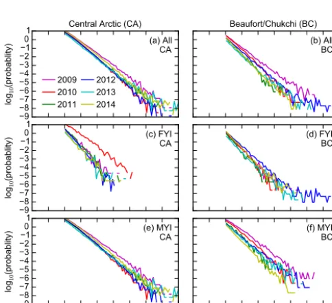
To investigate the tail of the distribution in more detail, Fig. 7 shows the distributions on a log-linear scale, clearly highlighting the exponential nature of the surface feature height distributions found in this study. An ordinary expo-nential distribution of sail heights was proposed by Wadhams (1980), which has been validated (to varying degrees) by fur-ther observations of sail/feature height (e.g. Tucker et al., 1979; Dierking, 1995; Martin, 2007; Rabenstein et al., 2010; Tan et al., 2012). As discussed earlier (Sect. 3), the feature heights presented here represent the peaks of the unique two-dimensional features, so a direct comparison between these
earlier studies (that detect the peak of the surface feature along a random (linear) profile) is not appropriate. Figure 7 demonstrates that a higher probability tail is prominent in the CA region in 2009 and 2014, to a lesser extent.
0 3 6 9 12 15 18 21 Probablity (%)
Central Arctic (CA) (a) All CA Beaufort/Chukchi (BC) (b) All BC 2009 2010 2011 2012 2013 2014 0 3 6 9 12 15 18 21 Probablity (%) (c) FYI
CA (d) FYIBC
0.0 0.5 1.0 1.5 2.0 2.5 3.0 Feature height (m) 0 3 6 9 12 15 18 21 Probablity (%) (e) MYI CA
0.0 0.5 1.0 1.5 2.0 2.5 3.0 Feature height (m)
(f) MYI BC
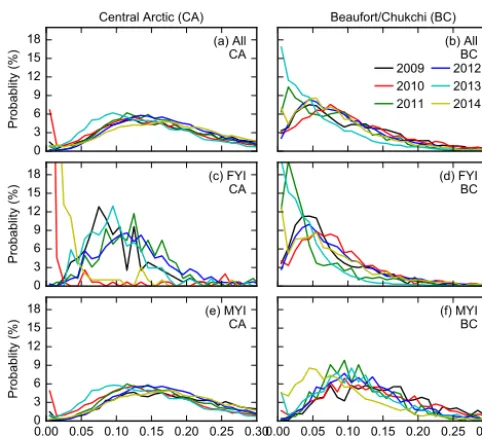
Figure 6.Probability distributions of the surface feature height,hf, (using a 20 cm elevation threshold) detected within the(a)Central Arctic and(b)Beaufort/Chukchi regions (shown in Fig. 5) and for the features estimated as FYI (candd) or MYI (eandf) using the OSI-SAF ice type mask described in Sect. 3. The bin width is 10 cm and the bin values are plotted as lines (joining each value) instead of steps for clarity. The solid (dashed) vertical lines show the mean (mode) of the distributions across each year. The statistics (mean, mode and standard deviation) are summarized in Table 2.
9 8 7 6 5 4 3 21 01 lo g10 (p ro ba bl ity )
Central Arctic (CA) (a) All CA 2009 2010 2011 2012 2013 2014 Beaufort/Chukchi (BC) (b) All BC 9 8 7 6 5 4 3 21 01 lo g10 (p ro ba bl ity
) (c) FYI
CA (d) FYIBC
0 1 2 3 4 5 6 7 8 9 Feature height (m) 9 8 7 6 5 4 3 21 01 lo g10 (p ro ba bl ity
) (e) MYI
CA
0 1 2 3 4 5 6 7 8 9 Feature height (m)
(f) MYI BC
Figure 7.As in Fig. 6 but for the surface feature height,hf, prob-ability distribution plotted on a log (base 10) scale. Only features higher than 2 m are shown to focus on the tail of the probability distributions.
than the CA region (a steeper gradient in the log-linear trend), as expected.
The feature height probability distributions for all fea-tures classified as either FYI or MYI (independent of region) are shown in the supplementary information (Fig. S6 in the Supplement). The distributions again show clear differences across ice types, with the mean feature height higher for the MYI (∼1.3 m) compared to the FYI (∼1.0 m), although the modal feature height is similar (∼0.45 m) across both ice types.
Table 3 provides statistics of the probability distributions of surface feature height, based on the higher (80 cm) ele-vation threshold processing. The distributions still show dif-ferences across regions, with a higher mean feature height in the CA (2.09±0.74 m) compared to the BC region (1.96±0.67 m), although this difference is significantly less than for the 20 cm results. Again, the mean modal feature height is similar (1.65 m for the CA and 1.55 m for the BC). These results further demonstrate the strong impact on the feature height distributions from the choice of cut-off eleva-tion.
4.1.2 Feature volume variability
Figure 8 shows maps of the mean surface feature volume per unit area (Vf) using the surface elevation threshold of 20 cm. Note that while these results include small (<100 m2) features,Vfexcluding small features showed similar results, with differences on the order of 0.01 m (not shown). It is worth noting again thatVf differs from the individual fea-ture height analysis as it represents the effective thickness of all surface features (total feature volume in the section spread over the entire swath area) within each 1 km ATM section. Figure 8, however, demonstrates a pattern consistent with the surface feature height analysis, including a higher
Vf(&0.15 m) in the CA region, and a lowerVf(.0.15 m) in
the BC region.Vfis greatest along the Greenland coastline (increasing up to∼0.3–0.4 m), especially towards northern Greenland (across most years) and along the eastern Green-land coast within the Fram Strait.Vfalso increases towards the Beaufort Sea coast in 2012. The regional variability in
Vf appears stronger than the feature height (hf) variability. Repeating the analysis for both the mean areal coverage and mean height of features (not shown) demonstrates a roughly equal contribution to the regional volume variability from each term (features increasing in area and height concur-rently).
To assess theVf variability across regions and ice type, Fig. 9 shows the probability distributions ofVf within the CA and BC regions, for all 1 km ATM sections and for the sections estimated as FYI or MYI. Statistics from these dis-tributions are summarized in Table 4. Note that as these data are based on the 1 km ATM sections (as opposed to individ-ual features), the data sampling is significantly reduced.
Figure 8.As in Fig. 5 but for the surface feature volume (per unit area),Vf.
Table 3.Surface feature height statistics, as in Table 2 but for the processing using an 80 cm threshold, with the results using all features in each region shown (not delineated by ice type).
Central Arctic Beaufort/Chukchi
Year Mean (m) Mode (m) No. (105) Mean (m) Mode (m) No. (105) 2009 2.22 (0.81) 1.75 1.11 2.11 (0.75) 1.55 0.28 2010 2.07 (0.71) 1.65 1.83 1.99 (0.65) 1.65 0.35 2011 2.07 (0.73) 1.55 1.69 1.91 (0.60) 1.55 0.07 2012 2.05 (0.72) 1.65 2.55 1.98 (0.69) 1.65 0.84 2013 2.08 (0.76) 1.55 1.13 1.93 (0.65) 1.55 0.44 2014 2.11 (0.76) 1.65 2.55 1.89 (0.59) 1.55 0.58 All 2.09 (0.74) 1.65 10.86 1.96 (0.67) 1.55 2.57
of sections classified as MYI is over an order of magni-tude higher across all years than the FYI (4.2×10⁴ com-pared to 0.2×10⁴), meaning the changing topography of the MYI is dominating the response of the Vf variability in the CA region (over changes in the MYI coverage), as demonstrated by the coincident variability in the MYI Vf. The FYI mean Vf (0.11±0.07 m) is lower than the MYI mean Vf (0.18±0.12 m) and again shows no discernible trend/pattern. The modal Vf in the CA experienced a more variable decline from 2009 to 2014 across both FYI and MYI distributions. In 2010 (all sections) and 2010/2014/all (FYI) the modalVfwas 0.01 m, highlighting the prevalence of (1 km) ATM sections with a negligibleVf(above the 20 cm elevation threshold). Note that this was not demonstrated in
the surface feature height analysis, as the size of the fea-tures is not taken into account. This highlights how the three-dimensional surface feature volume analysis presented is a more useful indicator of the total ice topography variability, compared to linear transects of peak feature heights, as dis-cussed in Sect. 3.1.4.
0 3 6 9 12 15 18
Probablity (%)
Central Arctic (CA) (a) All
CA
Beaufort/Chukchi (BC) (b) All
BC 2009 2010 2011
2012 2013 2014
0 3 6 9 12 15 18
Probablity (%)
(c) FYI
CA (d) FYIBC
0.00 0.05 0.10 0.15 0.20 0.25 0.30
Vf (per unit area, m) 0
3 6 9 12 15 18
Probablity (%)
(e) MYI CA
0.00 0.05 0.10 0.15 0.20 0.25 0.30
Vf (per unit area, m) (f) MYI
BC
Figure 9. Probability distributions of the surface feature volume (per unit area),Vf, (using a 20 cm elevation threshold) within the (a) Central Arctic and (b) Beaufort/Chukchi regions (shown in Fig. 8) from 2009 to 2014. The bin width is 1 cm. The statistics (mean and mode of each distribution) are summarized in Table 4.
in 2014, the MYI and FYI Vfare similar (0.09±0.07 m to 0.08±0.08 m). The number of sections has increased by a similar ratio (3) than the increase in features detected, sug-gesting consistency in the density of features detected.
4.1.3 Potential causes of feature height and volume variability
A recent study by Kwok (2015) provided estimates of the rel-ative contribution to sea ice thickness variability from con-vergence (dynamics) and melt (thermodynamics) north of Greenland and the Canadian Arctic Archipelago. The strong increase in bothhf andVfin the CA region between 2013 and 2014 found in this study is consistent with the strong increase in convergence-driven ice growth (within a similar region) during the preceding summer, estimated by Kwok (2015) using sea ice drift and assumptions of mass conser-vation. Strong ice convergence was also estimated by Kwok (2015) in December 2008, which may be linked to the high features observed in this study along the CA coastline in 2009. The Kwok (2015) study also showed that variability in the convergence-driven ice growth may be higher than ther-modynamic (melt-driven) changes, highlighting the impor-tant role of ice deformation variability in the Arctic sea ice mass balance.
In the BC region, the feature height and volume variabil-ity is driven more by variabilvariabil-ity in the presence of MYI. The presence of MYI in the Beaufort Sea (e.g. the tongue of MYI extending from the CA to the southern Beaufort Sea in 2012)
is the result of a complex interplay between the impact of the Beaufort Gyre on ice drift (e.g. Hutchings and Rigor, 2012; Petty et al., 2016) and the variable melt-out of ice in the Beaufort/Chukchi region (e.g. Hutchings and Rigor, 2012). The strong increase in the BC MYI coverage in 2014 has also coincided with an overall recovery of older ice across the Arctic since 2013 (see Fig. 4.3a in Perovich et al. (2015), based on ice age data from Tschudi et al., 2015). Both Till-ing et al. (2015) and Kwok and CunnTill-ingham (2015) showed an increase in Arctic sea ice volume in 2014, linked to the retention of MYI.
While our study provides information regarding the sur-face feature variability, the underside extension of the pres-sure ridge system, the keel, is thought to be significantly larger in size (e.g. Wadhams, 2000). Strub-Klein and Sudom (2012) recently compiled and analysed several ridge mor-phology data sets collected over the last few decades. They demonstrated that, on average, the maximum keel depth is around 4 times larger than the maximum sail height, while the keel width is around 6–7 times wider than the sail width. This suggests a keel volume up to ∼20–30 times larger than sail volume. The changes in surface feature volume,Vf, demonstrated in this study (±0.05 m) suggest, to a first-order approximation, total deformation variability up to∼1 m, if the keels are taken into account. This simple estimate as-sumes minimal impact from snow redistribution variability, which will act to reduce the magnitude of this estimate. Un-fortunately, detailed information regarding snow variability (spatial and temporal) over Arctic sea ice is lacking.
4.2 Sea ice topography as a function of coastline proximity
Table 4.Surface feature volume statistics taken from the probability distributions shown in Fig. 9. The value in the brackets (next to the means) equals 1 standard deviation of the relevant distribution. The third column (under each region) shows the number of 1 km ATM sections used in each distribution.
Central Arctic Beaufort/Chukchi
Year Mean (m) Mode (m) No. (104) Mean (m) Mode (m) No. (104) All 2009 0.19 (0.11) 0.12 0.42 0.11 (0.08) 0.04 0.24
2010 0.15 (0.09) 0.01 0.67 0.11 (0.08) 0.08 0.21 2011 0.17 (0.09) 0.12 0.78 0.08 (0.06) 0.01 0.10 2012 0.18 (0.11) 0.14 1.11 0.10 (0.07) 0.04 0.86 2013 0.15 (0.15) 0.10 0.66 0.06 (0.07) 0.01 0.86 2014 0.19 (0.13) 0.18 1.01 0.09 (0.07) 0.06 0.72 All 0.17 (0.12) 0.12 4.64 0.08 (0.07) 0.04 2.98
FYI 2009 0.10 (0.05) 0.08 0.02 0.07 (0.06) 0.04 0.13 2010 0.02 (0.06) 0.01 0.02 0.09 (0.09) 0.06 0.09 2011 0.12 (0.05) 0.12 0.02 0.05 (0.06) 0.01 0.05 2012 0.13 (0.06) 0.12 0.09 0.09 (0.07) 0.04 0.64 2013 0.10 (0.04) 0.10 0.02 0.04 (0.06) 0.01 0.58 2014 0.03 (0.04) 0.01 0.01 0.08 (0.08) 0.01 0.22 All 0.11 (0.07) 0.01 0.16 0.07 (0.07) 0.01 1.71
MYI 2009 0.21 (0.12) 0.12 0.30 0.16 (0.08) 0.08 0.05 2010 0.15 (0.09) 0.12 0.60 0.14 (0.07) 0.10 0.09 2011 0.18 (0.09) 0.12 0.71 0.12 (0.05) 0.10 0.03 2012 0.18 (0.11) 0.15 0.99 0.13 (0.07) 0.10 0.16 2013 0.15 (0.16) 0.10 0.58 0.11 (0.07) 0.11 0.16 2014 0.20 (0.13) 0.18 0.96 0.09 (0.07) 0.04 0.44 All 0.18 (0.12) 0.12 4.15 0.11 (0.07) 0.08 0.93
although the results also suggest significant spatial and tem-poral variability in the width of this BC landfast ice regime. A detailed analysis of specific IceBridge flight lines (in iso-lation) is therefore likely needed to detect and estimate the ice topography around the variable landfast ice edge.
In this study, we more broadly analyse the coastal depen-dency of the surface feature height,hf, and mean surface fea-ture volume,Vf, data presented in the previous section. Fig-ure 10 showshfrepresented by box and whisker plots, sepa-rated into coastline proximity bins (100 km wide) for the BC and CA regions. The coastal proximity data were presented in Sect. 2 and a map of the coastline proximity is given in the Supplement (Fig. S7). Note that less weight should be given to the BC results as there are much fewer data near to the coast (the period of 2012–2014 has the highest coverage of data near to the BC coastline). It is also worth noting that the CA coastal region (northern Greenland and the Canadian Archipelago) is dominated by MYI, whereas the BC coastal region (northern Canada and Alaska) shows greater interan-nual variability in the dominant ice type, as discussed previ-ously.
Despite the consistent presence of MYI over much of the CA region, Fig. 10 demonstrates a strong increase inhfwith increasing coastline proximity (in terms of the 25th, 50th 75th and 95th percentiles) up to 900 km away from the coast. The 0–100 km bin shows a significant fraction (∼5 %) of
fea-0.0
0.8
1.6
2.4
3.2
4.0
Feature height (m)
(a) Central Arctic
2009
2010
2011
2012
2013
2014
All
0
1
2
3
4
5
6
7
8
9
Distance to coast (100 km)
0.0
0.8
1.6
2.4
3.2
4.0
Feature height (m)
(b) Beaufort/Chukchi
tures higher than∼3.3 m, compared to the distance bins fur-ther from the coast. The results show moderate interannual variability, with 2009 showing higher features (compared to the other years) from 0 to 200 km from the coast, while 2014 shows higher features from 100 to 800 km from the coast, highlighting that the increase in surface feature height in 2014 manifested over much of the CA region, while in 2009, the high surface features were contained mostly along the CA coastline.
The BC region also demonstrates an increase in surface feature height with increasing coastline proximity, although this is mainly observed in the upper percentiles (75th and 95th) of the distributions. The median feature height across the 0–400 km percentile bins shows higher variability than the CA region. The 95th percentile results from 0 to 300 km are lowest in 2013, which may be due, in part, to the thin level ice sampled in the Chukchi Sea north of Point Hope in 2013 (Richter-Menge and Farrell, 2013). The feature heights also tend to increase (across most percentile ranges) at distances greater than 700 km away, which is likely due to the import of MYI from the CA into the northern Beaufort Sea.
The surface feature volume (per unit area), Vf, results, shown in Fig. 11, demonstrate a similar and perhaps more obvious coastline relationship. In the CA region, 2009 and 2014 show increases inVfcloser to the coastline, similar to the feature height results discussed previously. The median
Vfacross all distance bins shows greater interannual variabil-ity compared tohf. In the BC region, theVfincrease towards the coast (75th and 95th percentile) is much clearer than the
hfresults, and the interannual variability is again higher. This suggests that the three-dimensional surface feature volume data are a more useful measure of coastal topographic vari-ability compared to the surface feature heights, especially compared to data compiled from linear transects. Note that reducing the bin width to 10 km and analysing the coastline dependency on this smaller scale did not demonstrate any ob-vious landfast ice zone (a steep gradient in ice topography) across either region.
4.3 Relationship between sea ice thickness and surface feature variability
The relationship between sail height and sea ice thickness has been discussed in several previous studies of sea ice pres-sure ridging, with varying conclusions drawn. Tucker and Govoni (1981) were perhaps the first to observe the link be-tween sail heights and the thickness of the ice blocks from which they formed, which they assumed to be representative of the parent ice thickness. A square-root relationship was presented, which was validated by additional in situ obser-vations (Tucker et al., 1984) and the two-dimensional parti-cle modelling study of Hopkins (1998). More recently, Mar-tin (2007) found only a weak correlation between sail height and the parent ice thickness using a variety of linear surface profiling data sets and assuming a similar square-root
rela-0.0
0.1
0.2
0.3
0.4
0.5
0.6
V
f(p
er
u
ni
t a
re
a,
m
)
(a) Central Arctic
2009
2010
2011
2012
2013
2014
All
0
1
2
3
4
5
6
7
8
9
Distance to coast (100 km)
0.0
0.1
0.2
0.3
0.4
0.5
0.6
V
f(p
er
u
ni
t a
re
a,
m
)
(b) Beaufort/Chukchi
Figure 11.As in Fig. 10 but for the surface feature volume (per unit area),Vf.
Figure 12.Correlation between the mean IceBridge sea ice thick-ness and surface feature heighthf, averaged over 10 km along-track sections. The solid lines represent the least-squares fit, assuming a square-root relationship (hf=b
√
Hi), wherebis the calculated regression coefficient, andr is the correlation coefficient for all years of data.σris the standard error of the residuals (or root mean squared error) calculated using all years of data.
tionship. A stronger, but still only moderate correlation was found when a linear fit was assumed.
Figure 13.The 2015 surface feature height,hf, (top left) and the estimated sea ice thickness using the relationshiphf=0.72 √
Hi given in Fig. 12 (top right). The bottom left panel shows the quick-look IceBridge ice thickness results, and the bottom right panel shows the difference between the ice thickness estimated in this study and the derived IceBridge thickness (bottom right).
Figure 14.Surface feature aspect ratio,R, detected using a 20 cm elevation threshold (left) and 80 cm threshold (right) in 2012. The dark grey (light grey) background indicates regions where more than 80 % of the daily data within each year’s IceBridge sea ice campaign dates are estimated as MYI (FYI), while the medium grey indicates a mix of FYI and MYI. The red (blue) dashed lines represent the Central Arctic (Beaufort/Chukchi) regions used in this study.
and assumptions of hydrostatic equilibrium and thus implic-itly include the deformed and undeformed ice, meaning hf andHi are not truly independent variables. The regressions are therefore expected to differ from those presented in pre-vious analyses, that correlated the sail heights with the thick-ness of the ice blocks within the ridge (e.g. Tucker et al., 1984) or the level ice thickness directly (e.g. Martin, 2007). Our likely inclusion of snow drift features, and the expected thermodynamic/dynamic changes over time of surface fea-tures (we are not measuring the feafea-tures as they are formed) will also impact these correlations, and weaken the physical links to pressure ridging constraints. We therefore do not at-tempt a validation of the square-root relationship found in previous studies, but instead seek to quantify the relation-ship between the peak surface feature heights found in this study and the local (total) sea ice thickness. Our analysis is therefore more in line with the regressions presented in
Beck-ers et al. (2015), between the total ice (plus snow) thick-ness and their estimated surface roughthick-ness (introduced in Sect. 3). In that study, a strong (negligible) linear correla-tion was found over the deformed (drifting) sea ice, although these regressions were limited by their considerably lower spatial/temporal sampling compared to the data presented in this study.
The regressions between the surface feature height,hf, and the total ice thickness,Hi, are shown in Fig. 12. We exper-imented with both linear and square-root relationships us-ing a least-squares fit, and slightly stronger correlations were found with the latter. The square-root relationships also cross the origin and are thus more physically consistent (the lin-ear correlations without a variableyintercept were markedly weaker), so we decided to present and focus on the square-root regressions in this study,hf=b
√
The regression using all years of data (2009–2014) demon-strates strong correlation (r=0.72,b=0.72). The annual regressions (given in Fig. 12) show that the strongest cor-relation is observed in 2013 (r=0.81). Strong correlations are observed across all other years (r=0.67–0.76), except for 2009, where only a weak (r=0.35) correlation, and a regression parameter higher than average (b=0.86) was found. This may be due to the decreased ATM coverage in 2009, although Fig. 12 suggests that the ice thickness results were also skewed low compared to the relationships demon-strated across all other years. Note that changing the aver-aging length scale (5 and 20 km) resulted in weaker correla-tions. In general, the consistency of these regressions (similar
bvalue) across different years (2010–2014) suggests consis-tency in the response of the ice to dynamical forcing.
To demonstrate the potential utility of these findings, Fig. 13 shows the sea ice thickness from the derived Ice-Bridge product, and the sea ice thickness estimated using the surface feature height, hf, and the relationship hf=b
√
Hi
(both using the 10 km mean data). Here we use the recently released 2015 ATM data to calculate the surface feature height (not presented earlier), and the 2015 quick-look sea ice thickness data. A regression parameter ofb=0.72 was used based on the regression analysis across 2009–2014. The maps qualitatively show the close correspondence between the spatial variability in ice thickness across the CA and BC regions from both the IceBridge product and the ice thick-ness estimated from hf. Differences between observed and predicted ice thickness are up to ±2 m in some regions, although this is within range of the combined root mean squared error of the regression (1.10 m, given in Fig. 13) and the mean 10 km IceBridge thickness uncertainty of 0.8 m (calculated from the raw IceBridge uncertainty estimates across all years). In general, the results provide a useful means of understanding ice topography and thickness vari-ability in more detail, and demonstrate how the ice thickness estimates could provide a useful proxy for ice thickness, es-pecially in regions where measurements of leads, which are needed to calculate sea ice freeboard, are sparse.
4.4 Feature geometry and the potential for additional feature characterizations
As discussed in the introduction, sea ice topography is cru-cial for estimating atmospheric form drag over Arctic sea ice. Calculations of atmospheric form drag require estimates of the surface feature height (as presented in this study), along with the surface feature density (e.g. Arya, 1973; Tsama-dos et al., 2014). Linear profiling studies calculating atmo-spheric form drag (e.g. Castellani et al., 2014) simply mea-sure the spacing between unique surface features along the linear profile, assuming that the features are randomly ori-entated and sufficiently sampled for this assumption to be valid. Mock et al. (1972) showed that for randomly oriented ridges, the average ridge frequency,µ, and the average ridge
density (the ratio of the total length of ridges per unit area),
RD, are related viaµ=(2/π )RD. In contrast to linear pro-filing studies,RD can be calculated directly with these data asRD=PiLi/ Atot=Ltot/ Atot, where the sum is over all features within the total ice/swath area (given a fully con-centrated ice pack). Assuming an elliptically shaped feature, the length of the major axis of a specific feature can be es-timated asLi=√2π(RAsf)0.5, whereR=(Cp/ Cs)0.5is the degree of elongation of the feature, as mentioned in Sect. 3. An average spacing between features can then be estimated
fromRDasXf=π / (2RD).
A crucial factor in this calculation is the assumption of lin-ear features in the estimation of ridging density. Figure 14 shows the mean aspect ratio (R) of all features detected across 1 year (2012) using the 20 and 80 cm elevation cut-off thresholds. For the 20 cm elevation cut-off (as used through-out much of this study), the aspect ratio of all features ap-pears to be ∼2–2.5 : 1, while for the 80 cm threshold, the estimated aspect ratio is∼3–4 : 1. The assumption of linear-ity is somewhat arbitrary, but is clearly more questionable in the 20 cm case. We have decided not to present calculations of ridging density and form drag estimates as we believe a more thorough analysis is needed, which is beyond the scope of this current study. Understanding the surface feature ge-ometry variability, and linking this with estimates of feature density relevant to form drag parameterizations and also melt pond formation, will be a crucial next step in the utility of this unique, three-dimensional sea ice topography data set.
5 Conclusions
We have presented a detailed characterization and analysis of Arctic sea ice topography using high-resolution, three-dimensional surface elevation data from the Airborne To-pographic Mapper, flown as part of NASA’s Operation Ice-Bridge mission. Surface features in the sea ice cover (caused by ice deformation and/or snow redistribution) are detected using a newly developed feature-picking algorithm. We de-rive information regarding the individual height and volume (per unit area) of surface features from 2009 to 2014 within the Beaufort/Chukchi and Central Arctic regions, across both first-year and multi-year ice regimes.
es-pecially north of Greenland and the Canadian Archipelago. The coastal proximity results provide useful context regard-ing interannual variability in the location of surface topog-raphy features. A strong correlation between surface feature height and ice thickness (from the IceBridge sea ice prod-uct) is found, based on a square-root relationship. The con-sistency of these regressions across different years (2010– 2014) suggests consistency in the response of the ice to dy-namical forcing. Overall, the results allude to the importance of regional and interannual ice deformation variability in the total sea ice mass balance, and provide crucial information regarding the tail of the sea ice thickness distribution across the western Arctic.
While this study presents the use of IceBridge data to un-derstand the Arctic sea ice topography, future work will at-tempt to understand the impact of ice topography on esti-mates of atmospheric form drag. Another exciting prospect involves the extension of this analysis to Antarctic sea ice, where observations of the sea ice state are extremely lacking. Data availability
The IceBridge ATM data are available at https: //nsidc.org/data/ilatm1b/ (regular – wide swath) and http://nsidc.org/data/ilnsa1b (narrow swath). The IceBridge DMS images are available at http://nsidc.org/data/iodms1b. The IceBridge IDCSI4 and quick-look sea ice data are available at http: //nsidc.org/data/docs/daac/icebridge/evaluation_products/ seaice-freeboard-snowdepth-thickness-quicklook-index. html and http://nsidc.org/data/idcsi4.html respectively. The daily OSI-SAF ice type data are available at http://saf.met.no/p/ice/ and the nearest coastline prox-imity data are available at http://oceancolor.gsfc.nasa.gov/ cms/DOCS/DistFromCoast.
The data processing scripts used in this study have been made publicly available at http://www.github.com/akpetty/ ibtopo2016.git, and the derived data sets have been archived at https://zenodo.org/record/51569. The primary author may be contacted for any further data requests.
The Supplement related to this article is available online at doi:10.5194/tc-10-1161-2016-supplement.
Acknowledgements. This work was supported by the NASA
IceBridge Project Science Office, NASA grant NNX13AK36G, and the NOAA Ocean Remote Sensing Program. We acknowledge and sincerely appreciate the efforts of the various IceBridge team members who contributed to the collection, processing and archiving of the various data sets utilized in this study.
Edited by: C. Haas
References
Aaboe, S., Breivik, L-A., Sørensen, A., Eastwood, S., and Lavergne, T.: Global Sea Ice Edge and Type Product User’s Manual, Prod-uct OSI-403-b, EUMETSAT Ocean and Sea Ice Satellite Appli-cation Facility available at: http://saf.met.no/docs/osisaf_cdop2_ ss2_pum_ice-edge-type_v1p1.pdf, 2015.
Abdalati, W., Zwally, H., Bindschadler, R., Csatho, B., Farrell, S., Fricker, H., Harding, D., Kwok, R., Lefsky, M., Markus, T., Mar-shak, A., Neumann, T., Palm, S., Schutz, B., Smith, B., Spin-hirne, J., and Webb, C.: The ICESat-2 Laser Altimetry Mission, Proc. IEEE, 98, 735–751, doi:10.1109/JPROC.2009.2034765, 2010.
Arya, S. P. S.: Contribution of form drag on pressure ridges to the air stress on Arctic ice, J. Geophys. Res., 78, 7092–7099, doi:10.1029/JC078i030p07092, 1973.
Beckers, J. F., Renner, A. H. H., Spreen, G., Gerland, S., and Haas, C.: Sea-ice surface roughness estimates from air-borne laser scanner and laser altimeter observations in Fram Strait and north of Svalbard, Ann. Glaciol., 56, 235–244, doi:10.3189/2015AoG69A717, 2015.
Brooks, C., Beckley, M., Blair, J. B., and Hofton., M.: Ice-Bridge LVIS POS/AV L1B Corrected Position and Alti-tude Data, Version 1 [2009–2014], Boulder, Colorado USA: NASA DAAC at the National Snow and Ice Data Center, doi:10.5067/2NWNMDSG5EPJ, (updated 2015), 2012. Castellani, G., Lupkes, C., Hendricks, S., and Gerdes, R.:
Variabil-ity of Arctic sea ice topography and its impact on the atmo-spheric surface drag, J. Geophys. Res.-Oceans, 119, 6743–6762, doi:10.1002/2013JC009712, 2014.
Chelton, D. B., deSzoeke, R. A., Schlax, M. G., El Naggar, K., and Siwertz, N.: Geographical Variability of the First Baroclinic Rossby Radius of Deformation, J. Phys. Oceanogr., 28, 433–460, doi:10.1175/1520-0485(1998)028<0433:GVOTFB>2.0.CO;2, 1998.
Dierking, W.: Laser profiling of the ice surface topography during the Winter Weddell Gyre Study 1992, J. Geophys. Res., 100, 4807–4820, doi:10.1029/94JC01938, 1995.
Doble, M. J., Skourup, H., Wadhams, P., and Geiger, C. A.: The re-lation between Arctic sea ice surface elevation and draft: A case study using coincident AUV sonar and airborne scanning laser, J. Geophys. Res., 116, C00E03, doi:10.1029/2011JC007076, 2011. Dominguez, R.: IceBridge DMS L1B Geolocated and Orthorecti-fied Images, Version 1 [2009–2014], Boulder, Colorado, USA, NASA DAAC at the National Snow and Ice Data Center, doi:10.5067/OZ6VNOPMPRJ0, (updated 2015), 2010. Feltham, D. L.: Sea Ice Rheology, Annu. Rev. Fluid Mech., 40, 91–
112, doi:10.1146/annurev.fluid.40.111406.102151, 2008. Haas, C.: EM ice thickness measurements during GreenICE 2004
field campaign, GreenICE Deliverable D11, 2004.
Hibler, W. D., Weeks, W. F., and Mock, S. J.: Statistical aspects of sea ice ridge distributions, J. Geophys. Res., 77, 5954–5970, doi:10.1029/JC077i030p05954, 1972.
Hibler, W. D., Mock, S. J., and Tucker, W. B.: Classification and variation of sea ice ridging in the western Arctic basin, J. Geophys. Res., 79, 2735–2743, doi:10.1029/JC079i018p02735, 1974.
Hutchings, J. K. and Rigor, I. G.: Role of ice dynamics in anoma-lous ice conditions in the Beaufort Sea during 2006 and 2007, J. Geophys. Res., 117, C00E04, doi:10.1029/2011JC007182, 2012. Krabill, W. B, Abdalati, W., Frederick, E., Manizade, S., Martin, C., Sonntag, J., Swift, R., Thomas, R., and Yungel, J.: Aircraft laser altimetry measurement of elevation changes of the green-land ice sheet: technique and accuracy assessment, J. Geody-nam., 34, 357–376, doi:10.1016/S0264-3707(02)00040-6, 2002. Krabill, W. B.: IceBridge ATM L1B elevation and return strength, Version 2 [2009–2014], Boulder, Colorado USA: NASA DAAC at the National Snow and Ice Data Center, doi:10.5067/19SIM5TXKPGT, (updated 2015), 2013.
Krabill, W. B.: IceBridge Narrow Swath ATM L1B Elevation and Return Strength, Version 2., Boulder, Colorado USA: NASA DAAC at the National Snow and Ice Data Center, doi:10.5067/CXEQS8KVIXEI, (updated 2015), 2014.
Kurtz, N., Studinger, M. S., Harbeck, J., Onana, V., and Yi, D.: Ice-Bridge L4 Sea Ice Freeboard, Snow Depth, and Thickness, Ver-sion 1, Boulder, Colorado USA: NASA DAAC at the National Snow and Ice Data Center, doi:10.5067/G519SHCKWQV6, 2015.
Kurtz, N. T., Farrell, S. L., Studinger, M., Galin, N., Harbeck, J. P., Lindsay, R., Onana, V. D., Panzer, B., and Sonntag, J. G.: Sea ice thickness, freeboard, and snow depth products from Oper-ation IceBridge airborne data, The Cryosphere, 7, 1035–1056, doi:10.5194/tc-7-1035-2013, 2013.
Kwok, R.: Sea ice convergence along the Arctic coasts of Green-land and the Canadian Arctic Archipelago: Variability and extremes (1992–2014), Geophys. Res. Lett., 42, 7598–7605, doi:10.1002/2015GL065462, 2015.
Kwok, R. and Cunningham, G. F.: Variability of Arctic sea ice thick-ness and volume from CryoSat-2, Phil. Trans. Roy. Soc., 373, doi:10.1098/rsta.2014.0157, 2015.
Laxon, S. W., Giles, K. A., Ridout, A. L., Wingham, D. J., Willatt, R., Cullen, R., Kwok, R., Schweiger, A., Zhang, J., Haas, C., Hendricks, S., Krishfield, R., Kurtz, N., Farrell, S., and Davidson, M.: CryoSat-2 estimates of Arctic sea ice thickness and volume, Geophys. Res. Lett., 40, 732–737, doi:10.1002/grl.50193, 2013. Lensu, M.: The Evolution of Ridged Ice Fields, Ph.D. thesis, De-partment of Mechanical Engineering, Helsinki University of Technology, Helsinki, Finland, 140 pp., 2003.
Leonardi, S., Orlandi, P., Smalley, R. J., Djenidi, L., and Antonia, R. A.: Direct numerical simulations of turbulent channel flow with transverse square bars on one wall, J. Fluid Mech., 491, 229–238, doi:10.1017/S0022112003005500, 2003.
Mahoney, A. R., Eicken, H., Gaylord, A. G., and Gens, R.: Landfast sea ice extent in the Chukchi and Beaufort Seas: The annual cy-cle and decadal variability, Cold Reg. Sci. Technol., 103, 41–56, doi:10.1016/j.coldregions.2014.03.003, 2014.
Maneewongvatana, S. and Mount, D. M.: Analysis of approxi-mate nearest neighbor searching with clustered point sets, eprint arXiv:cs/9901013, 1999.
Martin, C. F., Krabill, W. B., Manizade, S. S., Russell, R. L., Sonntag, J. G., Swift, R. N., and Yungel, J. K.: Airborne to-pographic mapper calibration procedures and accuracy assess-ment, Tech. Rep. NASA/TM-2012-215891, 1–32, NASA, Cent. for AeroSpace Inform., Hanover, MD, 2012.
Martin, T.: Arctic sea ice dynamics: drift and ridging in numerical models and observations, Ph.D. thesis, Alfred Wegener Institute
for Polar and Marine Research, University of Bremen, Bremer-haven, 2007.
Martin, T., Steele, M., and Zhang, J.: Seasonality and long-term trend of Arctic Ocean surface stress in a model, J. Geophys. Res.-Oceans, 119, 1723–1738, doi:10.1002/2013JC009425, 2014. Maslanik, J., Stroeve, J., Fowler, C., and Emery, W.: Distribution
and trends in Arctic sea ice age through spring 2011, Geophys. Res. Lett., 38, L13502, doi:10.1029/2011GL047735, 2011. Mock, S. J., Hartwell, A. D., and Hibler, W. D.: Spatial aspects
of pressure ridge statistics, J. Geophys. Res., 77, 5945–5953, doi:10.1029/JC077i030p05945, 1972.
Newman, T., Farrell, S. L., Richter-Menge, J., Connor, L. N., Kurtz, N. T., Elder, B. C., and McAdoo, D.: Assessment of radar-derived snow depth over Arctic sea ice, J. Geophys. Res.-Oceans, 119, 8578–8602, doi:10.1002/2014JC010284, 2014.
Onana, V. D. P., Kurtz, N. T., Farrell, S. L., Koenig, L. S., Studinger, M., and Harbeck, J. P.: A sea ice Lead Detec-tion Algorithm for Use With High-ResoluDetec-tion Airborne Vis-ible Imagery, IEEE T. Geosci. Remote Sens., 51, 38–56, doi:10.1109/TGRS.2012.2202666, 2013.
Perovich, D. K. and Polashenski, C.: Albedo evolution of seasonal Arctic sea ice, Geophys. Res. Lett., 39, L08501, doi:10.1029/2012GL051432, 2012.
Perovich, D. K., Meier, W., Tschudi, M., Farrell, S. L., Gerland, S., and Hendricks, S.: Sea ice [in Arctic Report Card 2015], http: //www.arctic.noaa.gov/reportcard (last access: 26 May 2016), 2015.
Petty, A. A., Hutchings, J. K., Richter-Menge, J. A., and Tschudi, M.: Sea ice circulation around the Beaufort Gyre: The chang-ing role of wind forcchang-ing and the sea ice state, J. Geophys. Res., doi:10.1029/2011JC007231, in press, 2016.
Polashenski, C., Perovich, D., and Courville, Z.: The mechanisms of sea ice melt pond formation and evolution, J. Geophys. Res., 117, C01001, doi:10.1029/2011JC007231, 2012.
Rabenstein, L., Hendricks, S., Martin, T., Pfaffhuber, A., and Haas, C.: Thickness and surface-properties of different sea ice regimes within the Arctic Trans Polar Drift: Data from sum-mers 2001, 2004 and 2007, J. Geophys. Res., 115, C12059, doi:10.1029/2009JC005846, 2010.
Richter-Menge, J. A. and Farrell, S. L.: Arctic sea ice conditions in spring 2009-2013 prior to melt, Geophys. Res. Lett., 40, 5888– 5893, doi:10.1002/2013GL058011, 2013.
Soille, P. J. and Ansoult, M. M.: Automated basin delineation from digital elevation models using mathematical morphology, Sig-nal Process., 20, 171–182, doi:10.1016/0165-1684(90)90127-K, 1990.
Strub-Klein, L. and Sudom, D.: A comprehensive analysis of the morphology of first-year sea ice ridges, Cold Reg. Sci. Technol., 82, 94–109, doi:10.1016/j.coldregions.2012.05.014, 2012. Tan, B., Li, Z., Lu, P., Haas, C., and Nicolaus, M.: Morphology of
sea ice pressure ridges in the northwestern Weddell Sea in win-ter, J. Geophys. Res., 117, C06024, doi:10.1029/2011JC007800, 2012.
Thomas, D. N. and Dieckmann, G. S.: Sea Ice, 2 ed., Wiley-Blackwell, Hoboken, NJ, 2009.
Tilling, R. L., Ridout, A., Shepherd, A., and Wingham, D. J.: In-creased Arctic sea ice volume after anomalously low melting in 2013, Nature Geosci., 8, 643–646, doi:10.1038/ngeo2489, 2015. Timco, G. and Weeks, W.: A review of the engineering prop-erties of sea ice, Cold Reg. Sci. Technol., 60, 107–129, doi:10.1016/j.coldregions.2009.10.003, 2010.
Tsamados, M., Feltham, D. L., Schroeder, D., Flocco, D., Farrell, S. L., Kurtz, N., Laxon, S. W., and Bacon, S.: Impact of variable atmospheric and oceanic form drag on simulations of Arctic sea ice, J. Phys. Oceanogr., 44, 1329–1353, doi:10.1175/JPO-D-13-0215.1, 2014.
Tschudi, M., Fowler, C., and Maslanik, J.:EASE-Grid Sea Ice Age, Version 2., Boulder, Colorado USA: NASA National Snow and Ice Data Center Distributed Active Archive Center, doi:10.5067/1UQJWCYPVX61, 2015.
Tucker, W. B. and Govoni, J. W.: Morphological investigations of first-year sea ice pressure ridge sails, Cold Reg. Sci. Technol., 5, 1–12, doi:10.1016/0165-232X(81)90036-7, 1981.
Tucker, W. B., Weeks, W. F., and Frank, M.: Sea ice ridging over the Alaskan Continental Shelf, J. Geophys. Res., 84, 4885–4897, doi:10.1029/JC084iC08p04885, 1979.
Tucker, W. B., Sodhi, D. S., and Govoni, J. W.: Structure of first-year pressure ridge sails in the Prudhoe Bay region, in: The Alaskan Beaufort Sea, Academic Press, edited by: Reimnitz, P. W. B. M. S., 115–135, doi:10.1016/B978-0-12-079030-2.50012-5, 1984.
Wadhams, P.: A comparison of sonar and laser profiles along corre-sponding tracks in the Arctic Ocean, in: Sea Ice Processes and Models, edited by: Pritchard, R. S., 283–299, Univ. of Wash. Press, Seattle, Washington, 1980.
Wadhams, P.: Sea-ice topography of the Arctic Ocean in the region 70 degrees W to 25 degrees E, Phil. Trans. Roy. Soc., 302, 45–85, doi:10.1098/rsta.1981.0157, 1981.
Wadhams, P.: Ice in the Ocean, Gordon & Breach Science Publish-ers, Amsterdam, 2000.
Wadhams, P. and Davy, T.: On the spacing and draft distributions for pressure ridge keels, J. Geophys. Res., 91, 10697–10708, doi:10.1029/JC091iC09p10697, 1986.
Wadhams, P. and Horne, R. J.: An analysis of ice profiles obtained by submarine sonar in the Beaufort Sea, J. Glaciol., 25, 401–424, 1980.
Warren, S. G., Rigor, I. G., Untersteiner, N., Radionov, V. F., Bryaz-gin, N. N., Aleksandrov, Y. I., and Colony, R.: Snow Depth on Arctic Sea Ice, J. Climate, 12, 1814–1829, doi:10.1175/1520-0442(1999)012<1814:SDOASI>2.0.CO;2, 1999.