The operational methane retrieval algorithm for TROPOMI

(1)

www.atmos-meas-tech.net/9/5423/2016/ doi:10.5194/amt-9-5423-2016

The operational methane retrieval algorithm for TROPOMI

Haili Hu1, Otto Hasekamp1, André Butz2, André Galli3, Jochen Landgraf1, Joost Aan de Brugh1, Tobias Borsdorff1, Remco Scheepmaker1, and Ilse Aben1

1_{SRON Netherlands Institute for Space Research, Utrecht, the Netherlands}

2_{Deutsches Zentrum für Luft- und Raumfahrt e.V. (DLR), Institut für Physik der Atmosphäre, Oberpfaffenhofen, Germany} 3_{Physics Institute, University of Bern, Bern, Switzerland}

Correspondence to:Haili Hu ([email protected])

Received: 31 March 2016 – Published in Atmos. Meas. Tech. Discuss.: 13 April 2016 Revised: 24 October 2016 – Accepted: 26 October 2016 – Published: 9 November 2016

Abstract. This work presents the operational methane re-trieval algorithm for the Sentinel 5 Precursor (S5P) satel-lite and its performance tested on realistic ensembles of simulated measurements. The target product is the column-averaged dry air volume mixing ratio of methane (XCH4),

which will be retrieved simultaneously with scattering prop-erties of the atmosphere. The algorithm attempts to fit spec-tra observed by the shortwave and near-infrared channels of the TROPOspheric Monitoring Instrument (TROPOMI) spectrometer aboard S5P.

The sensitivity of the retrieval performance to atmospheric scattering properties, atmospheric input data and instrument calibration errors is evaluated. In addition, we investigate the effect of inhomogeneous slit illumination on the instrument spectral response function. Finally, we discuss the cloud fil-ters to be used operationally and as backup.

We show that the required accuracy and precision of<1 % for the XCH4 product are met for clear-sky measurements

over land surfaces and after appropriate filtering of difficult scenes. The algorithm is very stable, having a convergence rate of 99 %. The forward model error is less than 1 % for about 95 % of the valid retrievals. Model errors in the input profile of water do not influence the retrieval outcome notice-ably. The methane product is expected to meet the require-ments if errors in input profiles of pressure and temperature remain below 0.3 % and 2 K, respectively. We further find that, of all instrument calibration errors investigated here, our retrievals are the most sensitive to an error in the instrument spectral response function of the shortwave infrared channel.

1 Introduction

Methane (CH4) is the most important anthropogenic

green-house gas after carbon dioxide (CO2). While it occurs in

smaller concentrations, it has a higher global warming po-tential per molecule than CO2. An accurate understanding of

CH4 sources and sinks is essential for a reliable prediction

of climate change. Space-based measurements can provide continuous and global monitoring of CH4, leading to

much-needed improved constraints on the surface fluxes.

Several current and future satellite missions measure CH4

abundances in the Earth’s atmosphere. The SCanning Imag-ing Absorption spectroMeter for Atmospheric Cartogra-pHY (SCIAMACHY) aboard ENVISAT (Bovensmann et al., 1999) was the first space-based instrument to measure at-mospheric CH4with sensitivity down to the Earth’s surface.

Frankenberg et al. (2005) were the first to use these measure-ments to constrain CH4surface fluxes. After loss of contact

with ENVISAT in 2012, the Greenhouse gases Observing SATellite (GOSAT) is currently the only satellite measuring atmospheric CH4(Kuze et al., 2009). While GOSAT has a

higher sensitivity and spatial resolution than SCIAMACHY, it has a fairly low spatial sampling. In 2017, the TROPO-spheric Monitoring Instrument (TROPOMI) will be launched aboard the Sentinel 5 Precursor (S5P) satellite, and it will provide CH4measurements as one of its key products with

unprecedented high precision, spatial resolution and global daily coverage.

The common goal of the above-mentioned missions is to provide atmospheric CH4 concentrations with sufficient

(2)

strategy relies on measuring spectra of sunlight, backscat-tered by the Earth’s surface and atmosphere, in the shortwave infrared (SWIR) spectral range. Absorption features of CH4

molecules allow for retrieval of its atmospheric concentration with high sensitivity down to the Earth’s surface where the main CH4sources are located. The applicability of such

mea-surements for estimating source strengths, however, strongly depends on the precision and accuracy achieved. Residual systematic biases must be well below 1 % to facilitate in-verse modelling (Meirink et al., 2006; Bergamaschi et al., 2007, 2009).

Scattering by aerosols and cirrus is one of the major chal-lenges for retrievals of CH4from space-based SWIR

obser-vations. While contamination by optically thick clouds can be filtered out reliably, optically thin scatterers are much harder to detect, yet they still modify the light path of the observed backscattered sunlight. This can lead to underesti-mation or overestiunderesti-mation of the true CH4column if not

ap-propriately accounted for. The net light path effect strongly depends on the amount, size and height distribution of the scatterers as well as on the reflectance of the underlying sur-face (Aben et al., 2007; Gloudemans et al., 2008). Therefore, retrieval strategies rely on inferring the target gas concentra-tion either simultaneously with atmospheric scattering prop-erties or with a light path proxy.

Frankenberg et al. (2005) introduced the “proxy” approach for CH4retrieval from SCIAMACHY measurements around

1600 nm, by using the simultaneously retrieved CO2column

as a light path proxy. The proxy approach relies on the as-sumptions that scattering effects cancel in the ratio of the CH4column and the CO2column, and that a prior estimate

of the CO2column is sufficiently accurate to recalculate the

CH4column from the measured CH4/CO2ratio. In this case

scattering is ignored in the forward modelling. Further appli-cations of the proxy approach for CH4retrieval from

SCIA-MACHY are described by Frankenberg et al. (2008) and Schneising et al. (2011). For GOSAT, the proxy approach has been successfully applied by Parker et al. (2011) and Schep-ers et al. (2012).

Alternatively, scattering-induced light path modification can be taken into account by simultaneously inferring the at-mospheric CH4concentration and physical scattering

proper-ties of the atmosphere. Such “physics-based” methods have been developed for space-based CO2 and CH4

measure-ments from SCIAMACHY, GOSAT and the Orbiting Car-bon Observatory (OCO); see e.g. Connor et al. (2008); Butz et al. (2009); Reuter et al. (2010); O’Dell et al. (2012). The physics-based methods make use of the oxygen (O2) A-band

in the near-infrared (NIR) around 760 nm and absorption bands of the target absorber in the SWIR spectral range. The advantage of physics-based methods for CH4 retrieval

compared to proxy methods is that they do not depend on prior information on the CO2 column. On the other hand,

the physics-based algorithms are more complex and com-putationally expensive. In addition, they may be limited by

the information content of the measurement with respect to aerosol properties and related forward model errors in the de-scription of aerosols. A detailed comparison between the two methods for GOSAT is provided by Schepers et al. (2012).

TROPOMI has four spectral channels in the ultravi-olet (UV), visible (VIS), near-infrared (NIR) and short-wave infrared (SWIR), with spectral ranges of 270–320, 310–495, 675–775 and 2305–2385 nm, respectively. We use TROPOMI measurements in the NIR and SWIR for CH4

re-trievals. This spectral range does not allow for a light-path-proxy approach, and thus the effect of aerosols and cirrus needs to be accounted for by using a physics-based method as described above. The goal of this paper is to present the CH4

retrieval algorithm for TROPOMI and investigate its sensitiv-ity to algorithm assumptions, atmospheric input data and in-strument calibration errors and filtering criteria. To this end, we simulated realistic TROPOMI measurements for aerosol-and cirrus-loaded atmospheres under clear-sky aerosol-and cloudy conditions.

The outline of this paper is as follows. We start with the methodology in Sect. 2, giving an overview of the instru-ment, the retrieval algorithm and the methane data product. Then, a detailed error sensitivity study is presented in Sect. 3, based on methane retrievals on a clear-sky global ensemble of simulated spectra. In Sect. 4, a study of cloud filtering is performed on a TROPOMI orbit of simulated spectra that cover a realistic range of cloud parameters. Conclusions are presented in Sect. 5.

2 Methodology

The S5P satellite has a designed 7-year lifetime and will fly in a sun-synchronous orbit at 824 km altitude. Its single pay-load, TROPOMI, is a push-broom imaging spectrometer with a wide swath of 2600 km and a ground pixel of 7×7 km2 in exact nadir. Approximately, TROPOMI observes a full swath per second, which results in∼216 spectra per sec-ond. The instrument comprises two spectrometer modules, the first containing the UV, VIS and NIR spectral channels, and the second dedicated to the SWIR channel. We use the NIR and SWIR channels with spectral resolutions of 0.38 and 0.25 nm and spectral sampling ratios of 2.8 and 2.5, re-spectively (Veefkind et al., 2012). Since the NIR and SWIR detectors are incorporated in different instrument modules, the NIR spectra will be co-registered with the SWIR spec-tra before performing CH4retrievals. Examples of simulated

TROPOMI NIR and SWIR spectra are shown in Fig. 1. 2.1 The retrieval algorithm

The S5P operational CH4retrieval algorithm is based on

Re-moTeC, which was orginally developed for CO2 and CH4

(3)

mea-Figure 1.Simulated TROPOMI spectra in the NIR and SWIR channels for a scenario from the global ensemble; see Sect. 3.1. The scenario, located in a rural area in Utah (USA), is observed at nadir and SZA=50◦.

surements has been done by Butz et al. (2012), where a de-tailed description of the algorithm can be found. Here, we summarise the essentials and elaborate on the modifications made since then.

2.1.1 The forward model

The algorithm aims to infer the atmospheric state vector

x from spectral measurementsy in the NIR (757–774 nm) and SWIR (2305–2385 nm) ranges. This requires a forward modelFthat can accurately compute the measurement given the atmospheric state:

y=F(x)+ey+eF, (1)

whereey is the measurement noise error, andeF is the

for-ward model error. The forfor-ward model incorporates the lin-earised radiative transfer model LINTRAN (Schepers et al., 2014). LINTRAN simulates the radiance at the top of the at-mosphere ITOA on a fine internal spectral grid. The model needs a solar irradiance spectrum on the internal spectral grid as input, which is inferred from the daily solar measure-ments of TROPOMI using the deconvolution approach by van Deelen et al. (2007) and Wassmann et al. (2015). The simulated radiance measurement is obtained by a spectral convolution of ITOA with the instrument spectral response function (ISRF).

In addition to accuracy, an important requirement of the algorithm is computational speed. To be able to process TROPOMI’s huge number of measurements, the CPU time per retrieval has to be on the order of seconds. Our algo-rithm achieves this by, among other things, using the linear k-method for multiple scattering (Hasekamp and Butz, 2008). Single scattering is calculated line by line as it is computa-tionally less expensive. To our knowledge, our algorithm is among the fastest in use for CH4full-physics retrievals, with

an average CPU time of 7–10 s per retrieval (Hasekamp et al., 2016).

For a given model atmosphere, the forward model sim-ulates spectra of backscattered sunlight, taking absorption and scattering by molecules and particles into account. The model atmosphere is defined for 36 pressure-equidistant ver-tical layers, with the top at 0.1 hPa and bottom at the sur-face pressure psurf. We calculate psurf by interpolating the

meteorological surface pressure, from the European Centre for Medium-Range Weather Forecasts (ECMWF), on the sur-face elevation, from a digital elevation map (Danielson and Gesch, 2011; Farr et al., 2007). The absorbing trace gases of interest are O2in the NIR band, and CH4, H2O and CO in

the SWIR band. The first guess layer subcolumns of these gases are calculated from input profiles of CH4 and CO

(from the global chemical transport model TM5; Houwel-ing et al., 2014), and temperature, humidity and pressure profiles (from ECMWF forecast data). Molecular absorp-tion features are calculated using appropriate spectroscopic databases (Tran et al., 2006; Rothman et al., 2009; Scheep-maker et al., 2012). Here, we evaluate the absorption cross sections on a 72-layer pressure-equidistant grid to account for the strong temperature dependence and pressure depen-dence of the cross sections. Molecular scattering properties are given by Rayleigh theory. Particulate absorption and scat-tering are computed with Mie theory using tabulated aerosol properties by Dubovik et al. (2006).

In our algorithm, the aerosol type is characterised by the refractive index and size distribution. The complex refractive index is fixed atn=1.4−0.01iin the O2A-band andn=

(4)

The size distribution is described by a power-law function with size parameterα(e.g. Mishchenko et al., 1999):

n(r)=     

A, ifr≤r1.

A(r/r1)−α, ifr1< r≤r2.

0, ifr > r2,

(2)

wherer1=0.1 µm,r2=10 µm,r is the particle radius and A is a normalisation constant. The amount of aerosol and its vertical distribution is provided by the vertically inte-grated column number densityNaerand a normalised

Gaus-sian height distributionh(zk)withzkthe height of layerk:

h(zk)=Bexp

−4 ln 2(zk−zaer) 2

w2

,

wherew=2000 m,zaeris the central height andBis a

nor-malisation constant. Thus, in layerkwith thickness1zk, the

layer subcolumnnkis given by

nk=Naerh(zk)1zk.

Butz et al. (2010) suggest that the exact choice of the fixed-value parameters, such as the refractive indices or the width of the height distribution, does not affect the retrievals sig-nificantly. To support this claim, we have studied the effect of different values for the fixed-value aerosol parameters on our retrievals, and we arrive at the same conclusion; see Ap-pendix A.

We have modified the retrieval forward model with respect to Butz et al. (2012) to account for chlorophyll fluorescence emission in a simplified manner as described by Frankenberg et al. (2012). In short, scattering of the fluorescence emission is ignored, and solely the spectral shape and absorption fea-tures by oxygen (O2) are modelled. This allows fluorescence

to be treated as a simple additive term to the radiance before convolution with the ISRF. The surface emission at the top of the atmosphere (TOA) is then modelled as

Fs(λ)TOA=Fssurf,755(1−s(λ−755))e

−τ_O2(λ)/µ_, ₍₃₎

whereτO2(λ)is the vertical optical thickness of oxygen,µ is the cosine of the viewing zenith angle andλis the wave-length in nanometres.F_ssurf_,₇₅₅andsrepresent the chlorophyll emission at 755 nm and its spectral slope, respectively. 2.1.2 The state vector

The state vectorxconsists of 25 elements; see Table 1. The target is a 12-layer pressure-equidistant vertical profile of CH4 partial column number densities. The 12 retrieval

lay-ers are related to 36-layer model atmosphere by the shared interfaces; i.e. each retrieval layer is divided in three sublay-ers for the forward model calculations. Retrieved ancillary parameters are the total column number densities of H2O

and CO, three scattering parametersNaer,αandzaer(related

to amount, size and height), the surface albedo (constant-term and first-order spectral dependence1 and in the NIR and SWIR band), two terms to account for a spectral shift of the measurement (NIR and SWIR band) and two terms to account for chlorophyll fluorescence emission,F_ssurf_,₇₅₅and s(see Eq. 3). An overview of the state vector elements and their a priori values is given in Table 1. We note that for the operational methane retrievals, the a priori value forF_ssurf_,₇₅₅ will come from a dedicated fluorescence retrieval scheme based on the Fraunhofer lines. In this study however, we sim-ply took an a prioriF_ssurf_,₇₅₅=0 photons s−1m−2nm−1. Fur-ther, we would like to mention that our retrieved CO column should be regarded as a diagnostic for the CH4retrieval. The

official TROPOMI CO product has a dedicated retrieval al-gorithm described by Landgraf et al. (2016).

2.1.3 The inversion procedure

The state vector is found by inverting Eq. (1), where the in-verse method is based on a Philips–Tikhonov regularisation scheme (Phillips, 1962; Tikhonov, 1963). Regularisation is required because the inverse problem is ill-posed; i.e. the measurements y typically contain insufficient information to retrieve all state vector elements independently. Philips– Tikhonov regularisation aims to reduce contributions from measurement noise to the retrieved state vector while retain-ing valuable information. Because the forward modelF(x) is non-linear inx, the inversion is performed iteratively by a step-size-controlled Gauss–Newton scheme, where at each iteration step the forward model is linearised.

The inverse algorithm findsxby minimising the cost func-tion that is the sum of the least-squares cost funcfunc-tion and a side constraint weighted by the regularisation parameterγ according to

ˆ x=min

x

kSy−1/2(F(x)−y)||2+γkW(x−xa)||2

,

whereSyis the diagonal measurement error covariance

ma-trix, which contains the noise estimate.xais an a priori state

vector, andW is a diagonal weighting matrix that renders the side constraint dimensionless and ensures that only the CH4 parameters and the scattering parameters contribute to

its norm:Wjj=1/xa,jfor the CH4column number densities

and the three aerosol parameters, andWjj=10−7/xa,j for

all other state vector elements. The latter are thus retrieved in a least-squares sense. For determiningγ, the L-curve cri-terion (Hansen, 1998) is applied in the baseline algorithm. However,γ may be fine-tuned later using real observations.

(5)

Table 1.State vector elements and their a priori values or references to source.

State vector element A priori value (units)

CH4subcolumns in 12 vertical layers TM5 (cm−2)

CO total column TM5 (cm−2)

H2O total column derived from ECMWF specific humidity (cm−2)

Aerosol columnNaer derived from aerosol optical thickness=0.1 at 760 nm (cm−2)

Aerosol size parameterα 3.5 (–)

Aerosol height parameterzaer 5000 (m)

Lambertian surface albedo in the NIR band maximum of measured reflectance in the NIR band (–) First-order spectral dependence surface albedo in the NIR band 0 (–)

Lambertian surface albedo in the SWIR band maximum of measured reflectance in the SWIR band (–) First-order spectral dependence surface albedo in the SWIR band 0 (–)

Spectral shift NIR 0 (nm)

Spectral shift SWIR 0 (nm)

Fluorescence emission at 755 nmF_ssurf_,₇₅₅ 0 (photons s−1m−2nm−1)

Fluorescence spectral slopes 0 (–)

2.2 The CH4data product

Although we retrieve methane inn=12 sublayers, there is virtually no profile information in the measurement. The de-gree of freedom of signal of the retrieved methane profile is about 1. Therefore, the methane data product is given as a column-averaged dry air mixing ratio XCH4. This quantity

is obtained from the methane entries of the retrieved state vectorxithrough

XCH4=

n

X

i=1

xi/Vair,dry, (4)

whereVair,dryis the dry air column (calculated from

meteoro-logical input surface pressure and the water vapour profile). To interpret the retrieved XCH4correctly, one also needs

the column averaging kernel Acol that describes the

sensi-tivity of the retrieved CH4 column to changes to the true

methane profile (see Rodgers, 2000, for details):

Acol,i=

∂

n

P

i=1 xi

∂xtrue,i

. (5)

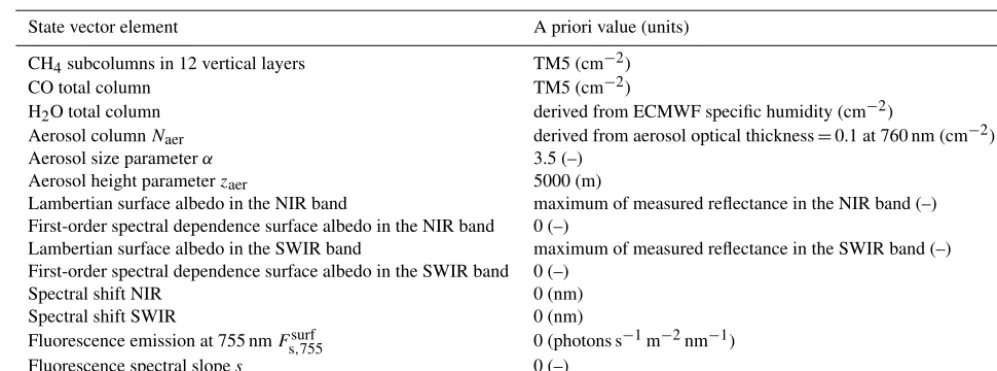
As an example, in Fig. 2 we show the column averaging ker-nel corresponding to the methane retrieval performed on the simulated spectra of Fig. 1. We see that the column averaging kernel is around 1 in the lower atmosphere. From Eq. (5) it is clear that the closerAcolis to 1, the more the retrieved

col-umn represents the true colcol-umn (see also Eq. 6). This illus-trates that the retrieval of methane columns from the SWIR has a nearly ideal sensitivity to methane in the troposphere and the tropospheric boundary layer.

For validation and interpretation purposes it is important to realise that the retrieved XCH4is related to the true methane

profilextrueand the a priori profilexaas

XCH4 =

n

X

i=1

Acol,ixtrue,i+(1−Acol,i)xa,i/Vair,dry

+ 1XCH4,F+1XCH4,y, (6)

where1XCH4,F is the bias caused by forward model

er-rors, and1XCH4,y is the retrieval noise due to measurement

noise. The standard deviation of the retrieval noise, i.e. the precisionσXCH4, follows from the error covariance matrix Sx, which describes the effect of measurement noise on the

retrieved parameters (see e.g. Rodgers, 2000, Sect. 4.3):

σXCH4= q

Pn i=1

Pn j=1Sx,i,j

Vair,dry

. (7)

Together with XCH4 and Acol, the precision σXCH4 is given in the main data product. Note that for simulations, the bias1XCH4,Fcan be calculated from Eq. (6), since all other

terms are either known from the simulations or calculated by the retrieval algorithm. In Sect. 3, we evaluate1XCH4,F, 1XCH4,y and their sensitivity to input errors.

2.3 Data filtering

(6)

Figure 2.Column averaging kernel for a typical methane retrieval. The retrieval was performed using the simulated NIR and SWIR spectra in Fig. 1.

2.3.1 A priori filtering

For operational cloud filtering, measurements from the Vis-ible Infrared Imaging Radiometer Suite (VIIRS) aboard the Suomi-NPP satellite will be used. S5P is foreseen to oper-ate in loose formation with Suomi-NPP, meaning that both missions observe the same ground scene with a time delay of about 5 min. In case VIIRS data are not available, we have developed a backup cloud filter using H2O retrievals from the

weak and strong absorption band, assuming a non-scattering atmosphere. Here we make use of the fact that clouds and aerosols will modify the optical path length in the two bands differently due to the different absorption strengths (Taylor et al., 2016; Frankenberg, 2014). Thus, there will be a dif-ference between the H2O column retrieved from the strong

band and the H2O column retrieved from the weak band in

the presence of clouds.

Based on tests with simulations, we chose 2329–2334 nm as the weak absorption band and 2367–2377 nm as the strong absorption band (see also Scheepmaker et al., 2016). In Fig. 3, we show the absorption features of H2O in the SWIR

range and highlighted the proposed weak and strong ab-sorption band. Because the weak-band and the strong-band retrievals are differently affected by scattering, the ratio

|H2Oweak−H2Ostrong|

H2Ostrong is strongly correlated with cloud contami-nation. Scenes in which this ratio exceeds a certain threshold can be flagged as cloudy and filtered out. Based on a realistic ensemble of synthetic measurements (see Sect. 4), we find that a threshold of 0.08 filters out most cloudy scenes and keeps most of the clear-sky scenes. However, a direct cloud filter based on VIIRS data is shown to be superior to this indirect two-band cloud approach. Therefore, the two-band

cloud filter will only be used as backup when VIIRS data are unavailable.

Figure 3.Simulated reflectance spectrum showing the absorption features of H2O in the SWIR spectral range for the same scenario as in Fig. 1. The red shaded area represents the weak absorption band, while the blue area represents the strong absorption band of H₂O. The difference between the water column retrieved from the weak and strong band is used for the backup cloud filter.

Further, before performing any CH4 retrievals, we filter

out cases with solar zenith angle (SZA) larger than 70◦, and viewing zenith angle (VZA) larger than 50◦. These thresh-olds have been derived from simulations and shall be fine-tuned after launch using real observations.

2.3.2 A posteriori filtering

Butz et al. (2012) identified an a posteriori filter based on retrieved scattering parameters: SWIR aerosol optical thick-nessτswirat 2350 nm, size parameterαand height parameter zaer. Following this work, we filter out retrievals with τswir·zaer

α >120 m.

This indicates that the retrieval algorithm has difficulties with scenes that have optically thick scattering layers of large par-ticles at high altitude. Additionally, we filter out cases with retrieved albedo in the SWIR band smaller than 0.02. More a posteriori filters (e.g. based on goodness of fit) will be de-termined after launch using real observations.

3 Sensitivity studies

Here, we evaluate the sensitivity of the retrieved XCH4

(7)

envisioned to be within 2 % and the product precision to be within 0.6 % (Veefkind et al., 2012). Accuracy is defined as the mean deviation from the truth, and precision is the varia-tion due to random processes such as instrument noise. More recently, the requirements have been slightly reformulated as 1 % bias and 1 % precision (Hasekamp et al., 2016). From the 1 % bias, 0.8 % is reserved for forward model errors and 0.6 % for instrument-related errors.

3.1 Synthetic measurements: the global ensemble

We performed detailed sensitivity studies of the CH4

algo-rithm on a global ensemble of simulated spectra consist-ing of land-only, clear-sky scenes on a 2.79◦×2.8125◦ lat-itude×longitude grid. This ensemble is, to a large extent, identical to the one used by Butz et al. (2012). It contains re-alistic aerosol- and cirrus-loaded scenes for 4 days, one per season. The treatment of aerosols and cirrus in the simula-tions is far more complex than in the retrieval forward model, where only one effective aerosol type is considered; see Sect. 2.1.1. For the simulations, the aerosol physical prop-erties and vertical distributions are derived from the global aerosol model ECHAM5-HAM (Stier et al., 2005) for five different chemical species and on a superposition of seven log-normal size distributions. The aerosol optical thickness is derived from MODIS observations (Remer et al., 2005). Fur-thermore, the simulations contains cirrus with optical thick-ness and vertical distribution based on CALIOP measure-ments (Winker et al., 2007). Finally, the surface albedo in the NIR is taken from the MODIS land albedo product in the 841–876 nm channel. For the albedo in the SWIR, the SCIA-MACHY surface albedo product at 2350 nm is used (Schri-jver et al., 2009). For simplicity, we assume a constant sur-face albedo within the NIR and SWIR band in our simula-tions. We expect no difficulties to fit a more realistic spectral dependent surface albedo based on our experience with real GOSAT data. We refer to Figs. 2 and 3 of Butz et al. (2012) for the geographical distribution of the total optical thickness and surface albedo, respectively, used in the simulations. The measurements are simulated for the nadir viewing direction and a solar zenith angle that is representative of TROPOMI with an overpass time of 13:30 local time. We have 8633 sim-ulated measurements in total.

While Butz et al. (2012) only investigated the scattering-induced error, we increased the inconsistency between the simulation forward model and the retrieval forward model model. We have attempted to include the most important con-tributions to the forward model error, except for errors due to the underlying spectroscopic database, which have been investigated elsewhere; see Galli et al. (2012) and Checa-Garcia et al. (2015). The simulations were computed using a line-by-line radiative transfer model, whereas the retrieval method uses the linear k-method. In addition, the simulations have a higher vertical and spectral resolution than used in the retrieval. Furthermore, we have added chlorophyll

fluores-cence emission. In the simulations, fluoresfluores-cence is modelled to have a double Gaussian spectral shape (Guanter et al., 2010), which is different from the linear spectral shape as-sumed in the retrieval forward model (see Eq. 3). As in the retrieval scheme, we neglect scattering of fluorescence emis-sion for simplicity. The fluorescence at the TOA then be-comes

Fs(λ)=Fs,755



 X

i=1,2 Aie

−(λ−_{λi )}2

σ_i2



e

−τ_O2(λ)/µ_. ₍₈₎

For the parametersA1,A2,λ1,λ2,σ1andσ2, we use the same

values as in Frankenberg et al. (2012). We only included flu-orescence emission for scenes in the global ensemble with albedoNIR/albedoSWIR>5 as a rough selection criterion for

regions with vegetation.

After convolving the simulated TOA radiance with the ISRF, the spectra are superimposed with instrument noise from the TROPOMI noise model (Tol et al., 2011). For the NIR, the noise consists solely of shot noise, while for the SWIR, the noise is composed of both shot noise and a signal-independent term. The corresponding continuum signal-to-noise ratios are 500 in the NIR and 100 in the SWIR for a ref-erence scene with surface albedoAs=0.05, viewing zenith

angle VZA=0◦and solar zenith angle SZA=70◦.

The baseline performance of the operational CH4

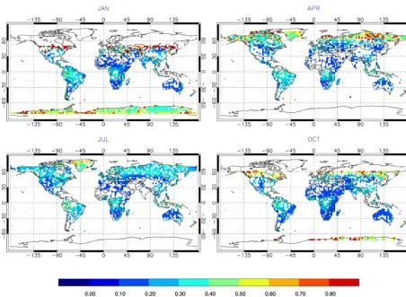
algo-rithm is tested on the simulated global ensemble described above. In Fig. 4, we show a world map of the bias1XCH4,F

before and after applying the a posteriori filters based on re-trieved scattering parameters and albedo. Note that the er-ror due to measurement noise1XCH4,y has been subtracted

from the total XCH4 error. This is a random error and is

evaluated separately in Sect. 3.3.1 In Fig. 5, the cumulative probability distribution of the absolute XCH4retrieval error

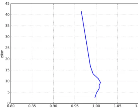
is shown (blue line). We get a convergence rate of 99 %, and 53 % of the converged retrievals pass the filters. Finally, 94 % of the valid retrievals have an absolute error<1 %. In Fig. 5, we also plotted the cumulative probability distribution in case fluorescence emission is not fitted (red line). Then, we have a convergence rate of 95 and 92 % of the valid retrievals have an error<1 %. Thus our retrieval results are improved by fit-ting fluorescence, which is why we have included this in the baseline.

(8)

(9)

Figure 5.Cumulative probability distribution of the absolute XCH4 forward model error for the baseline retrieval (blue line) and for the case that fluorescence emission is not fitted (red line).

3.2 Sensitivity to atmospheric input data

We investigated the effect of imprecise atmospheric input from TM5 and ECMWF on the CH4retrievals. The results

are summarised in Fig. 6. 3.2.1 A priori CH4profile

For the baseline performance test in Sect. 3.1 we used the true profile of methanextrueas the a priori profile for the

re-trievals. The bias1XCH4,F as defined in Eq. (6) should not

depend on the choice of the a priori profile because this ef-fect is accounted for by the averaging kernel. To test this, we take the zonal mean as the a priori profile, where we aver-aged over all longitudes within a 2.79◦ latitude bin, with a column deviation up to±2 %. To illustrate the effect on the global ensemble, we evaluate the root mean square (rms) of the XCH4bias (i.e. the total XCH4error minus the

contribu-tion due to noise) of all retrievals that pass the a posteriori filters. Figure 6 (first panel, blue line) shows that the a pri-ori CH4does not influence the retrieval accuracy, in terms of

the rms of the XCH4 bias, nor the stability, in terms of the

convergence rate or number of valid retrievals. 3.2.2 A priori H2O profile

To investigate the sensitivity to errors on the assumed H2O

profile, we follow the same procedure as in Sect. 3.2.1. The error on the prior H2O profile is established in the same way

as for CH4, i.e. by taking a normalised zonal mean profile per

latitude bin. Note that for H2O, there is an additional (minor)

influence on the retrieval of XCH4through the dry air

col-umn. The H2O column error is varied up to±10 %. Figure 6

(left panel, red line) shows that the prior H2O profile has

neg-ligible influence on the rms of the XCH4bias, increasing it

with<0.01 %. There is a small effect on the convergence rate, reducing it from 99 to 97 % and leading to a reduction of valid retrievals from 53 to 50 %. We note that taking a zonal mean profile for H2O represents a worst case in terms

of accuracy for the specific humidity of ECMWF. 3.2.3 Pressure

An erroneous pressure affects the retrieval of XCH4in two

ways: first of all, through the pressure dependence of the cross sections and, secondly, through the retrieved air col-umn that is used to convert the CH4total column to the dry

air mixing ratio, XCH4. The latter will introduce a retrieval

error of the same magnitude as the pressure error. To evalu-ate the net effect of a pressure error, the prior pressure profile is perturbed with a scaling factor up to±0.3 %, correspond-ing to|1Psurf| ≈3 hPa. We expect a better accuracy from the

ECMWF surface pressure together with the digital elevation map (Salstein et al., 2007; Danielson and Gesch, 2011; Farr et al., 2007). Figure 6 (right panel, blue line) shows that the increase in the rms of the XCH4 bias is<0.15 %. There is

no visible effect on the stability of the algorithm. 3.2.4 Temperature

An error in the temperature will propagate to the XCH4

re-trievals though the temperature dependence of the cross sec-tions. To investigate this effect, the temperature profile is off-set up to±2 K. Figure 6 (right panel, blue line) shows that the increase in the rms of the XCH4 bias is<0.15 %. There is a small effect on the stability of the algorithm, reducing the convergence rate to 97 % and the number of valid retrievals to 47 %.

3.3 Sensitivity to instrument errors

We investigated the effect of different possible instrument and calibration errors on the CH4retrievals. The results are

summarised in Table 2. Below we discuss each effect sepa-rately.

3.3.1 Signal-to-noise ratio

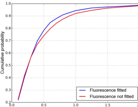
The simulated spectra include instrument noise as described in Sect. 3.1. The precision is given by the standard devi-ation of the retrieval noise σXCH4; see Eq. (7). The world map in Fig. 7 shows the precision relative to the retrieved XCH4. Typically the precision is better than the accuracy.

(10)

Figure 6.Influence of errors in atmospheric input on the accuracy (panels 1 and 2) and stability (panels 3 and 4) of XCH4retrievals. The upper and lowerxaxes refer to perturbations. Accuracy refers to the XCH4bias, and stability refers to the fraction of converged and valid retrievals. The profiles of methane and water have been perturbed in panels 1 and 3; the pressure and temperature profiles have been perturbed in panels 2 and 4.

3.3.2 Instrument spectral response function

The synthetic measurements were created by convolving the underlying line-by-line spectra with a Gaussian ISRF with a full width half maximum (FWHM) of 0.38 nm in the NIR band and 0.25 nm in the SWIR band. The mission require-ments state that the ISRF shall be known within 1 % of its maximum (Langen et al., 2011). This is achieved approxi-mately by varying the FWHM by 1 %. Table 2 give the re-sults for retrievals with an assumed error in the FWHM. We find that the retrievals are mostly sensitive to the accuracy of the ISRF in the SWIR band, leading to an increase of the rms XCH4bias from 0.56 % (baseline) to 0.67 %. We note that of

all the instrument errors investigated here, the ISRF gives the largest error contribution to the methane retrievals. Thus, our study indicates that accurate calibration of the ISRF should have high priority.

3.3.3 Spectral calibration

According to the instrument requirements, the centre wave-lengths of spectral channels are known within 2 pm (picome-tres). For our global ensemble, a spectral shift of 2 pm has negligible effect on the error characteristics. Here, we eval-uate the effect of a wavelength shift of 1/20 of the spectral sampling distance, i.e. 10 and 5 pm for the NIR and SWIR band, respectively. The reference retrieval fits a spectral shift. To test this fitting option, the synthetic spectra were shifted with a constant wavelength:

λk,meas=λk+1λ, (9)

where λk is the real wavelength, λk,meas is the measured

wavelength at pixelkand1λthe spectral shift. In Table 2, re-sults are given for the case that a spectral shift is not fitted and is fitted (between brackets). When fitted, the performance is as good as for the reference retrieval, i.e. simulations

with-out an error in the spectral position. This is as expected and indicates that the spectral shift fitting is robust.

Optionally a wavelength-dependent shift, 1λsqueeze, can

be fitted. To test this fitting option, the synthetic wavelength grid was “squeezed”:

λk,meas=λk+1λsqueeze×(λk−λmid)/(λend−λmid), (10)

whereλendandλmidare the wavelengths at the end and

mid-dle of the band, respectively. Table 2 shows the performance of retrievals with this assumed error on the measured wave-length grid. Since a spectral squeeze is a second-order effect and has a much smaller impact on the XCH4retrievals than a

spectral shift, it is not fitted in the baseline. However, our re-sults show that, if needed, the option to fit a spectral squeeze can be used reliably.

3.3.4 Radiometric offset: additive factor

The effect of an unknown systematic offset in the Earth radi-ance is investigated. The offsets in the NIR and SWIR bands are independently varied with±0.1 % of the continuum. Ta-ble 2 shows the effect of a radiometric offset to the XCH4

retrievals. We note that a radiometric offset in the SWIR band causes a larger XCH4error than an offset in the NIR

band. The latter is partly compensated by the retrieved fluo-rescence.

3.3.5 Radiometric gain: multiplicative factor

(11)

be-Figure 7.Relative precision of XCH4due to the instrument noise for the a posteriori filtered data set for the clear-sky ensemble in Fig. 4.

Table 2.Effect of instrument calibration errors on convergence rate, fraction of valid retrievals after filtering and rms values of XCH₄bias and precision for the global ensemble. Note that all sensitivities include the baseline forward model error, caused mainly by aerosol and cirrus scattering. The terms between brackets are for the cases where the relevant quantity is also retrieved. For each instrument calibration error, multiple simulation runs were performed with all combinations of errors in NIR and SWIR channels. The results shown here correspond to the runs with poorest performance in terms of the rms error.

Convergence Valid retrievals rms of XCH4bias rms of XCH4precision

Baseline 99 % 53 % 0.56 % 0.43 %

1FWHMNIR= −1 % 99 % 53 % 0.56 % 0.43 %

1FWHMSWIR= −1 % 99 % 49 % 0.67 % 0.44 %

1FWHMNIR/SWIR= −1 % 99 % 49 % 0.67 % 0.44 %

1λshift,NIR= −10 pm 97 % 48 % 0.57 % 0.42 %

1λshift,SWIR=5 pm 99 % 50 % 0.99 % 0.42 %

1λshift,NIR/SWIR= −10/5 pm 99 % (99 %) 46 % (53 %) 1.02 % (0.56 %) 0.41 % (0.43 %)

1λsqueeze,NIR=10 pm 99 % 53 % 0.56 % 0.42 %

1λsqueeze,SWIR=5 pm 99 % 52 % 0.62 % 0.42 %

1λsqueeze,NIR/SWIR=10/5 pm 96 % (99 %) 53 % (53 %) 0.63 % (0.56 %) 0.42 % (0.43 %)

Ioffset,NIR= −0.1 % 99 % 53 % 0.57 % 0.43 %

Ioffset,SWIR=0.1 % 99 % 50 % 0.58 % 0.43 %

Ioffset,NIR/SWIR= −0.1/0.1 % 99 % 50 % 0.59 % 0.43 %

GNIR=1.02 99 % 53 % 0.56 % 0.43 %

GSWIR=1.02 99 % 53 % 0.58 % 0.42 %

(12)

Figure 8.Methane bias due to heterogenous slit illumination for spatially varying surface reflection over a marsh scene at Siberia close to the river Ob at latitude 62.8◦N and longitude 72.1◦E. Measurement simulations are performed with the instrument model by Landgraf et al. (2016) for an instantaneous field of view of 3.4 km across the slit and 7.0 km along the slit.

tween surface albedo and aerosols has a negligible impact for gain errors<2 %.

3.4 Heterogenous slit illumination

For the two-dimensional TROPOMI push-broom spectrom-eter, light in across-slit dimension is dispersed by the in-strument grating in order to spectrally resolve the received signal. The along-slit direction is aligned across flight di-rection to achieve the desired spatial resolution. For a ho-mogeneous illumination of the instrument slit, the spectral instrument response is characterised extensively during the pre-flight calibration of the TROPOMI instrument, and it is used as baseline to simulate the TROPOMI radiometric measurement in our retrieval. In space, however, the instru-ment slit will be illuminated inhomogeneously due to ground scene heterogeneities on scales smaller than the instrument’s field of view. Inhomogeneous illumination across the slit leads to a distortion of the ISRF as described by Noël et al. (2012), Caron et al. (2014) and Landgraf et al. (2016), and it can affect the retrieval accuracy of the TROPOMI methane product. Small-scale heterogeneities of the ground scene are generally caused by spatial variations of surface reflection and by broken clouds. Because of our strict cloud filtering, spatial variations in surface reflection are the only cause of methane retrieval biases due to inhomogeneous slit illumi-nation. To evaluate the effect of surface scene heterogeneity on our XCH4product, we employ the instrument model

de-scribed by Landgraf et al. (2016) for both the NIR and SWIR bands of our retrieval. Furthermore, we use a high spatial resolution MODIS albedo map for the 50×50 km2 marsh region in central Siberia with structures in the surface reflec-tion due to ponds, shown in Fig. 8. Depending on the scene heterogeneity in the flight direction, the XCH4error shows

an oscillation structure with a maximum amplitude≤0.4 %, a standard deviation of 0.12 % and a mean error of−0.01 %. For a particular temporal and spatial sampling of the scene,

a pseudo-random scatter is introduced to the XCH4product.

This means that overall the effect can be considered small. One may consider this error as a limitation when interpret-ing very localised sources in surroundinterpret-ings of heterogenous surface reflection, but for most applications some averaging either in time or space will be done, which reduces this error.

4 Cloud filtering

The global ensemble from Butz et al. (2012) as used in Sect. 3 cannot be used to evaluate the cloud filters, because it consists purely of cloud-free scenes. Therefore, the cloud filters are tested using a new ensemble of synthetic measure-ments, which also include scenes with water clouds. 4.1 Synthetic measurements: the TROPOMI test orbit

To test the performance of the proposed backup cloud fil-ter, we have constructed synthetic TROPOMI L1B radiance spectra for an entire orbit that passes over Africa. We used realistic viewing geometries from a TROPOMI orbit simu-lator provided by the Royal Netherlands Meteorological In-stitute (KNMI). The meteorological data are from ECMWF. We used CO and CH4model profiles from TM5 (Houweling

(13)

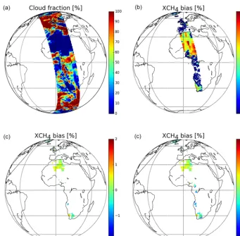
Figure 9.Simulations of a TROPOMI orbit. Panel(a)shows MODIS cloud fraction resampled on the orbit’s ground pixels. Panel(b)gives the XCH4bias of all processed pixels that converged. Panel(c)and(d)give XCH4bias of the valid retrievals after cloud filtering with MODIS data and the backup cloud filter, respectively. Here, we also applied the a posteriori filter based on retrieved scattering parameters and albedo.

Table 3.Error statistics of XCH4retrievals from the L1B orbit using different cloud filters in comparison to the global clear-sky orbit. The performance of the MODIS filter is expected to be comparable with the operational cloud filter using VIIRS data.

Retrievals with

|XCH4error|<1 % |XCH4error|<0.5 % rms of XCH4bias rms of XCH4precision

Global clear-sky ensemble 94 % 78 % 0.56 % 0.43 %

L1B orbit with MODIS filter 96 % 80 % 0.56 % 0.31 %

L1B orbit with backup cloud filter 94 % 79 % 0.71 % 0.27 %

the surface pressure, also provided by MODIS. The cloud properties are collocated in time and space to the TROPOMI orbit and used in the measurement simulation. For fractional clouds, the independent-pixel approximation is used to com-bine the cloudy and clear-sky parts of the scene. For refer-ence, the cloud fraction used in the simulations is shown in Fig. 9, upper left. We note that 28 % of the TROPOMI ground pixels are fully cloud-free for this test orbit. Glob-ally, one would expect, on average, 20 % cloud-free pix-els (Krijger et al., 2007). Resampling of the auxiliary data

on the TROPOMI ground pixels has been performed us-ing the Multi-Instrument Preprocessor (MIPrep) developed at SRON.

4.2 Performance of cloud filters

First, we show the performance of the XCH4 retrievals

(14)

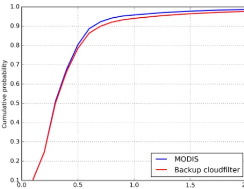
Figure 10. Cumulative probability distribution of the absolute XCH4 bias for the simulated level 1b orbit. Cloud-contaminated measurements are filtered using MODIS data (blue line) or the backup cloud filter (red line).

cloud-contaminated measurements lead to large XCH4errors

(>2 %).

Assuming that we have cloud data from VIIRS, we would then be able to filter out the cloudy pixels almost perfectly. To illustrate the effect, we filtered out pixels with cloud fraction >0.02 in Fig. 9, lower left. Note that in this case we have also applied a posteriori filtering based on retrieved scattering pa-rameters and albedo. One is then left with valid retrievals of

∼3 % of all simulations in the test orbit.

In comparison, the performance of the backup cloud filter based on the difference between the H2O column retrieved

from strong and weak bands (see Sect. 2.3) is shown in Fig. 9, lower right. The backup cloud filter removes most cloudy pixels, but some remain. In Table 3 and Fig. 10, the statistics of XCH4retrievals on the orbit are summarised. After cloud

filtering with MODIS data (representative of operational VI-IRS data), the results for the test orbit are comparable to the clear-sky global ensemble. However, the backup cloud filter is less effective. The rms of the XCH4bias is then 0.71 %

in-stead of the 0.56 % that is expected for the operational VIIRS cloud mask.

5 Conclusions

This paper describes the algorithm baseline of the operational methane retrievals from the S5P measurements. The level 2 product includes the column-averaged dry air mixing ratio XCH4, the column averaging kernel and the noise standard

deviation. In order to account for the effect of aerosols and cirrus, the algorithm developed retrieves the methane column simultaneously with effective scattering parameters related to particle amount, size and height distribution. The choice

of scattering parameters reflects the information content of the measurements as closely as possible. The retrieval al-gorithm uses the radiance and irradiance measurements in the SWIR 2305–2385 nm band and additionally in the NIR band between 757 and 774 nm (O2 A-band). The forward

model of the retrieval algorithm uses online radiative trans-fer calculations, fully including multiple scattering in an ef-ficient manner. Absorption cross sections of the relevant at-mospheric trace gases and optical properties of aerosols are calculated from lookup tables. The inversion is performed using Phillips–Tikhonov regularisation in combination with a reduced-step-size Gauss–Newton iteration scheme.

To test the developed algorithm we generated two en-sembles of simulated measurements that cover the range of scenes that will likely be encountered by the S5P instru-ment: one clear-sky global ensemble and one test orbit con-taining cloud-contaminated measurements. Overall, the al-gorithm developed performs well in correcting for the ef-fect of aerosols and cirrus clouds on the retrieved XCH4. For

both ensembles,∼80 % of the cases have an XCH4 error <0.5 % and∼95 % have an error<1 %. To achieve this, it is necessary to apply a priori filtering of cloud-contaminated scenes and a posteriori filtering based on retrieved parame-ters. We illustrated the performance of the proposed backup cloud filter based on retrievals of H2O from weak and strong

absorption bands in the SWIR under the assumption of a non-scattering atmosphere. It should be noted that the cloud filter based on S5P measurements itself is less efficient than the VIIRS cloud mask for water clouds.

Apart from forward model errors induced by aerosols, we also studied effects of model errors in temperature, pressure and water vapour profiles. We expect to stay within product requirements for errors in input profiles of water, pressure and temperature below 10 %, 0.3 % and 2 K, respectively. Another relevant source of errors to the CH4 data product

could be spectroscopic errors. This has been studied in detail by Galli et al. (2012) and Checa-Garcia et al. (2015). Note that a study is ongoing to improve the spectroscopic data for TROPOMI’s SWIR spectral range (Loos et al., 2015). Con-cerning instrument errors, we found that the most critical er-ror source is an erer-ror in the ISRF in the SWIR band. To con-clude, we have shown that for a compliant instrument, our algorithm provides a methane product that meets the require-ments.

6 Data availability

(15)

Table A1.Effect of fixed-value aerosol parameters on convergence rate, fraction of valid retrievals after filtering and rms values of XCH₄ bias and precision for the global ensemble. See text for values used in the baseline run.

Convergence Valid retrievals rms of XCH4bias rms of XCH4precision

Baseline 99 % 53 % 0.56 % 0.43 %

n=1.37−0.0005i 99 % 47 % 0.60 % 0.40 %

n=1.55−0.02i 99 % 53 % 0.57 % 0.43 %

w=1 km 99 % 53 % 0.56 % 0.42 %

w=3 km 99 % 53 % 0.56 % 0.41 %

Appendix A: Sensitivity of retrievals to fixed-value aerosol parameters

Our retrieval algorithm retrieves three effective aerosol pa-rameters, namely total column, size parameter and central height. Other aerosol parameters are assumed to be fixed, such as the refractive indices nand widthwof the aerosol layer (i.e. FWHM of Gaussian height distribution). The val-ues in the baseline retrieval are fixed atnNIR=1.4−0.01i, nSWIR=1.47−0.008i andw=2 km, respectively. To

(16)

Acknowledgements. We thanks M. Sneep (The Royal Netherlands Meteorological Institute, KNMI) and S. Houweling (SRON) for providing us with auxiliary data needed to simulate TROPOMI measurements. This research has been funded in part by the TROPOMI national programme from the Netherlands Space Office (NSO). André Butz is supported by the Deutsche Forschungs-gemeinschaft through the Emmy Noether Programme, grant BU2599/1-1 (RemoteC).

Edited by: J. Kim

Reviewed by: two anonymous referees

References

Aben, I., Hasekamp, O., and Hartmann, W.: Uncertainties in the space-based measurements of CO2columns due to scattering in the Earth’s atmosphere, J. Quant. Spectrosc. Ra., 104, 450–459, doi:10.1016/j.jqsrt.2006.09.013, 2007.

Bergamaschi, P., Frankenberg, C., Meirink, J. F., Krol, M., Dentener, F., Wagner, T., Platt, U., Kaplan, J. O., KöRner, S., Heimann, M., Dlugokencky, E. J., and Goede, A.: Satellite chartography of atmospheric methane from SCIA-MACHY on board ENVISAT: 2. Evaluation based on inverse model simulations, J. Geophys. Res.-Atmos., 112, D02304, doi:10.1029/2006JD007268, 2007.

Bergamaschi, P., Frankenberg, C., Meirink, J. F., Krol, M., Vil-lani, M. G., Houweling, S., Dentener, F., Dlugokencky, E. J., Miller, J. B., Gatti, L. V., Engel, A., and Levin, I.: Inverse modeling of global and regional CH4 emissions using SCIA-MACHY satellite retrievals, J. Geophys. Res.-Atmos., 114, D22301, doi:10.1029/2009JD012287, 2009.

Bovensmann, H., Burrows, J. P., Buchwitz, M., Frerick, J., Noël, S., Rozanov, V. V., Chance, K. V., and Goede, A. P. H.: SCIA-MACHY: Mission Objectives and Measurement Modes, J. At-mos. Sci., 56, 127–150, 1999.

Butz, A., Hasekamp, O. P., Frankenberg, C., and Aben, I.: Retrievals of atmospheric CO_2 from simulated space-borne measurements of backscattered near-infrared sunlight: accounting for aerosol effects, Appl. Opt., 48, 3322, doi:10.1364/AO.48.003322, 2009. Butz, A., Hasekamp, O. P., Frankenberg, C., Vidot, J., and Aben, I.: CH4 retrievals from space-based solar backscatter measure-ments: Performance evaluation against simulated aerosol and cirrus loaded scenes, J. Geophys. Res.-Atmos., 115, D24302, doi:10.1029/2010JD014514, 2010.

Butz, A., Galli, A., Hasekamp, O., Landgraf, J., Tol, P., and Aben, I.: {TROPOMI} aboard Sentinel-5 Precursor: Prospec-tive performance of {CH4} retrievals for aerosol and cirrus loaded atmospheres, Remote Sens. Environ., 120, 267–276, doi:10.1016/j.rse.2011.05.030, 2012.

Caron, J., Sierk, B., Bezy, J., Loescher, A., and Meijer, Y.: The CarnoSat candidate mission: radiometric and specteral perfor-mances over spatially heterogeneouse scenes, International Con-ference on Space Optics, ICOS, 7–10 October 2014, Tenerife, Spain, 2014.

Checa-Garcia, R., Landgraf, J., Galli, A., Hase, F., Velazco, V. A., Tran, H., Boudon, V., Alkemade, F., and Butz, A.: Mapping spec-troscopic uncertainties into prospective methane retrieval errors

from Sentinel-5 and its precursor, Atmos. Meas. Tech., 8, 3617– 3629, doi:10.5194/amt-8-3617-2015, 2015.

Connor, B. J., Boesch, H., Toon, G., Sen, B., Miller, C., and Crisp, D.: Orbiting Carbon Observatory: Inverse method and prospec-tive error analysis, J. Geophys. Res.-Atmos., 113, D05305, doi:10.1029/2006JD008336, 2008.

Danielson, J. and Gesch, D.: Global multi-resolution terrain eleva-tion data 2010 (GMTED2010), US Geological Survey Open-File Report, 2011-1073, 26, 2011.

Dubovik, O., Holben, B., Eck, T. F., Smirnov, A., Kaufman, Y. J., King, M. D., Tanré, D., and Slutsker, I.: Variability of Absorption and Optical Properties of Key Aerosol Types Observed in World-wide Locations, J. Atmosp. Sci., 59, 590–608, doi:10.1175/1520-0469(2002)059<0590:VOAAOP>2.0.CO;2, 2002.

Dubovik, O., Sinyuk, A., Lapyonok, T., Holben, B. N., Mishchenko, M., Yang, P., Eck, T. F., Volten, H., MuñOz, O., Veihelmann, B., van der Zande, W. J., Leon, J.-F., Sorokin, M., and Slutsker, I.: Application of spheroid models to account for aerosol particle nonsphericity in remote sensing of desert dust, J. Geophys. Res.-Atmos., 111, D11208, doi:10.1029/2005JD006619, 2006. Farr, T. G., Rosen, P. A., Caro, E., Crippen, R., Duren, R.,

Hens-ley, S., Kobrick, M., Paller, M., Rodriguez, E., Roth, L., Seal, D., Shaffer, S., Shimada, J., Umland, J., Werner, M., Oskin, M., Bur-bank, D., and Alsdorf, D.: The Shuttle Radar Topography Mis-sion, Rev. Geophys., 45, RG2004, doi:10.1029/2005RG000183, 2007.

Frankenberg, C.: OCO-2 IMAP-DOAS preprocessor algorithm theoretical basis document, Report, Jet Propulsion Laboratory, California Institute of Technology, Pasadena, CA, USA, avail-able at: http://disc.sci.gsfc.nasa.gov/OCO-2/documentation/ oco-2-v5/IMAP_OCO2_ATBD_prelaunch.pdf, 2014.

Frankenberg, C., Platt, U., and Wagner, T.: Retrieval of CO from SCIAMACHY onboard ENVISAT: detection of strongly pol-luted areas and seasonal patterns in global CO abundances, At-mos. Chem. Phys., 5, 1639–1644, doi:10.5194/acp-5-1639-2005, 2005.

Frankenberg, C., Warneke, T., Butz, A., Aben, I., Hase, F., Spi-etz, P., and Brown, L. R.: Pressure broadening in the 2ν3band of methane and its implication on atmospheric retrievals, At-mos. Chem. Phys., 8, 5061–5075, doi:10.5194/acp-8-5061-2008, 2008.

Frankenberg, C., O’Dell, C., Guanter, L., and McDuffie, J.: Remote sensing of near-infrared chlorophyll fluorescence from space in scattering atmospheres: implications for its retrieval and interfer-ences with atmospheric CO2retrievals, Atmos. Meas. Tech., 5, 2081–2094, doi:10.5194/amt-5-2081-2012, 2012.

Galli, A., Butz, A., Scheepmaker, R. A., Hasekamp, O., Landgraf, J., Tol, P., Wunch, D., Deutscher, N. M., Toon, G. C., Wennberg, P. O., Griffith, D. W. T., and Aben, I.: CH4, CO, and H2O spec-troscopy for the Sentinel-5 Precursor mission: an assessment with the Total Carbon Column Observing Network measure-ments, Atmos. Meas. Tech., 5, 1387–1398, doi:10.5194/amt-5-1387-2012, 2012.

Gloudemans, A. M. S., Schrijver, H., Hasekamp, O. P., and Aben, I.: Error analysis for CO and CH4total column retrievals from SCIAMACHY 2.3 µm spectra, Atmos. Chem. Phys., 8, 3999– 4017, doi:10.5194/acp-8-3999-2008, 2008.

(17)

flu-orescence retrieval from spaceborne high-resolution spectrome-try in the O2-A and O2-B absorption bands, J. Geophys. Res.-Atmos., 115, D19303, doi:10.1029/2009JD013716, 2010. Hansen, P.: Rank-Deficient and Discrete Ill-Posed Problems:

Nu-merical Aspects of Linear Inversion, Mathematical Modeling and Computation, Society for Industrial and Applied Mathematics, 263 pp., doi:10.1137/1.9780898719697, 1998.

Hasekamp, O., Hu, H., Galli, A., Tol, P., Landgraf, J., and Butz, A.: Algorithm Theoretical Baseline Document for Sentinel-5 Precursor methane retrieval, Report, SRON netherlands Insti-tute for Space Research, available at: http://www.tropomi.eu/ sites/default/files/files/SRON-S5P-LEV2-RP-001_TROPOMI_ ATBD_CH4_v1p0p0_20160205.pdf, 2016.

Hasekamp, O. P. and Butz, A.: Efficient calculation of intensity and polarization spectra in vertically inhomogeneous scattering and absorbing atmospheres, J. Geophys. Res-Atmos., 113, D20309, doi:10.1029/2008JD010379, 2008.

Houweling, S., Krol, M., Bergamaschi, P., Frankenberg, C., Dlugo-kencky, E. J., Morino, I., Notholt, J., Sherlock, V., Wunch, D., Beck, V., Gerbig, C., Chen, H., Kort, E. A., Röckmann, T., and Aben, I.: A multi-year methane inversion using SCIAMACHY, accounting for systematic errors using TCCON measurements, Atmos. Chem. Phys., 14, 3991–4012, doi:10.5194/acp-14-3991-2014, 2014.

Krijger, J. M., van Weele, M., Aben, I., and Frey, R.: Technical Note: The effect of sensor resolution on the number of cloud-free observations from space, Atmos. Chem. Phys., 7, 2881–2891, doi:10.5194/acp-7-2881-2007, 2007.

Kuze, A., Suto, H., Nakajima, M., and Hamazaki, T.: Ther-mal and near infrared sensor for carbon observation Fourier-transform spectrometer on the Greenhouse Gases Observing Satellite for greenhouse gases monitoring, Appl. Opt., 48, 6716, doi:10.1364/AO.48.006716, 2009.

Landgraf, J., aan de Brugh, J., Scheepmaker, R., Borsdorff, T., Hu, H., Houweling, S., Butz, A., Aben, I., and Hasekamp, O.: Car-bon monoxide total column retrievals from TROPOMI short-wave infrared measurements, Atmos. Meas. Tech., 9, 4955– 4975, doi:10.5194/amt-9-4955-2016, 2016.

Langen, J., Meijer, Y., Brinksma, E., Veihelmann, B., and Ingmann, P.: GMES Sentinels 4 and 5 mission requirements document, Mrd, European Space Agency (ESA), 2011.

Loos, J., Birk, M., Wagner, G., Didier, M., Kassi, S., Vasilchenko, S., Campargue, A., Hase, F., Orphal, J., Perrin, A., Tran, H., Coudert, L., Dufour, G., Eremenko, M., Cuesta, J., Daumont, L., Rotger, M., Bigazzi, A., and Zehner, C.: Spectroscopic Database for TROPOMI/Sentinel-5 Precursor, ESA ATMOS 2015 confer-ence proceedings (ESA SP-735), 8–12 June 2015, Heraklion, Greece, 2015.

Meirink, J. F., Eskes, H. J., and Goede, A. P. H.: Sensitivity analysis of methane emissions derived from SCIAMACHY observations through inverse modelling, Atmos. Chem. Phys., 6, 1275–1292, doi:10.5194/acp-6-1275-2006, 2006.

Mishchenko, M. I., Geogdzhayev, I. V., Cairns, B., Rossow, W. B., and Lacis, A. A.: Aerosol retrievals over the ocean by use of channels 1 and 2 AVHRR data: sensitivity anal-ysis and preliminary results, Appl. Opt., 38, 7325–7341, doi:10.1364/AO.38.007325, 1999.

Noël, S., Bramstedt, K., Bovensmann, H., Gerilowski, K., Bur-rows, J. P., Standfuss, C., Dufour, E., and Veihelmann, B.:

Quan-tification and mitigation of the impact of scene inhomogeneity on Sentinel-4 UVN UV-VIS retrievals, Atmos. Meas. Tech., 5, 1319–1331, doi:10.5194/amt-5-1319-2012, 2012.

O’Dell, C. W., Connor, B., Bösch, H., O’Brien, D., Frankenberg, C., Castano, R., Christi, M., Eldering, D., Fisher, B., Gunson, M., McDuffie, J., Miller, C. E., Natraj, V., Oyafuso, F., Polonsky, I., Smyth, M., Taylor, T., Toon, G. C., Wennberg, P. O., and Wunch, D.: The ACOS CO2retrieval algorithm – Part 1: Description and validation against synthetic observations, Atmos. Meas. Tech., 5, 99–121, doi:10.5194/amt-5-99-2012, 2012.

Parker, R., Boesch, H., Cogan, A., Fraser, A., Feng, L., Palmer, P. I., Messerschmidt, J., Deutscher, N., Griffith, D. W. T., Notholt, J., Wennberg, P. O., and Wunch, D.: Methane observations from the Greenhouse Gases Observing SATellite: Comparison to ground-based TCCON data and model calculations, Geophys. Res. Lett., 38, L15807, doi:10.1029/2011GL047871, 2011.

Phillips, D. L.: A Technique for the Numerical Solution of Cer-tain Integral Equations of the First Kind, J. ACM, 9, 84–97, doi:10.1145/321105.321114, 1962.

Remer, L. A., Kaufman, Y. J., Tanré, D., Mattoo, S., Chu, D. A., Martins, J. V., Li, R.-R., Ichoku, C., Levy, R. C., Kleidman, R. G., Eck, T. F., Vermote, E., and Holben, B. N.: The MODIS Aerosol Algorithm, Products, and Validation, J. Atmos. Sci., 62, 947–973, doi:10.1175/JAS3385.1, 2005.

Reuter, M., Buchwitz, M., Schneising, O., Heymann, J., Bovens-mann, H., and Burrows, J. P.: A method for improved SCIA-MACHY CO2retrieval in the presence of optically thin clouds, Atmos. Meas. Tech., 3, 209–232, doi:10.5194/amt-3-209-2010, 2010.

Rodgers, C.: Inverse Methods for Atmospheres: Theory and Prac-tice, World Scientific Publishing, Singapore, 240 pp., 2000. Rothman, L., Gordon, I., Barbe, A., Benner, D. C., Bernath, P. F.,

Birk, M., Boudon, V., Brown, L. R., Campargue, A., Champion, J.-P., Chance, K., Coudert, L. H., Dana, V., Devi, V. M., Fally, S., Flaud, J.-M., Gamache, R. R., Goldman, A., Jacquemart, D., Kleiner, I., Lacome, N., Lafferty, W. J., Mandin, J.-Y., Massie, S. T., Mikhailenko, S. N., Miller, C. E., Moazzen-Ahmadi, N., Nau-menko, O. V., Nikitin, A. V., Or- phal, J., Perevalov, V. I., Perrin, A., Predoi-Cross, A., Rins- land, C. P., Rotger, M., Šimeˇcková, M., Smith, M. A. H., Sung, K., Tashkun, S. A., Tennyson, J., Toth, R. A., Vandaele, A. C., and Vander Auwera, J: The HI-TRAN 2008 molecular spectroscopic database, J. Quant. Spec-trosc. Ra., 110, 533–572, doi:10.1016/j.jqsrt.2009.02.013, avail-able at: http://hitran.org, 2009.

Salstein, D., Ponte, R. M., and Cady-Pereira, K.: Uncertainties in atmospheric surface pressure fields from global analyses, J. Geo-phys. Res., 113, D14107, doi:10.1029/2007JD009531, 2007. Scheepmaker, R. A., Frankenberg, C., Galli, A., Butz, A.,

Schri-jver, H., Deutscher, N. M., Wunch, D., Warneke, T., Fally, S., and Aben, I.: Improved water vapour spectroscopy in the 4174–4300 cm−1 region and its impact on SCIAMACHY HDO/H2O measurements, Atmos. Meas. Tech., 6, 879–894, doi:10.5194/amt-6-879-2013, 2013.

(18)

Schepers, D., Guerlet, S., Butz, A., Landgraf, J., Frankenberg, C., Hasekamp, O., Blavier, J.-F., Deutscher, N. M., Griffith, D. W. T., Hase, F., Kyro, E., Morino, I., Sherlock, V., Suss-mann, R., and Aben, I.: Methane retrievals from Greenhouse Gases Observing Satellite (GOSAT) shortwave infrared mea-surements: Performance comparison of proxy and physics re-trieval algorithms, J. Geophys. Res.-Atmos., 117, D10307, doi:10.1029/2012JD017549, 2012.

Schepers, D., aan de Brugh, J. M. J., Hahne, P., Butz, A., Hasekamp, O. P., and Landgraf, J.: LINTRAN v2.0: A lin-earised vector radiative transfer model for efficient simula-tion of satellite-born nadir-viewing reflecsimula-tion measurements of cloudy atmospheres, J. Quant. Spectrosc. Ra., 149, 347–359, doi:10.1016/j.jqsrt.2014.08.019, 2014.

Schneising, O., Buchwitz, M., Reuter, M., Heymann, J., Bovens-mann, H., and Burrows, J. P.: Long-term analysis of car-bon dioxide and methane column-averaged mole fractions re-trieved from SCIAMACHY, Atmos. Chem. Phys., 11, 2863– 2880, doi:10.5194/acp-11-2863-2011, 2011.

Schrijver, H., Gloudemans, A. M. S., Frankenberg, C., and Aben, I.: Water vapour total columns from SCIAMACHY spectra in the 2.36 µm window, Atmos. Meas. Tech., 2, 561–571, doi:10.5194/amt-2-561-2009, 2009.

Stier, P., Feichter, J., Kinne, S., Kloster, S., Vignati, E., Wilson, J., Ganzeveld, L., Tegen, I., Werner, M., Balkanski, Y., Schulz, M., Boucher, O., Minikin, A., and Petzold, A.: The aerosol-climate model ECHAM5-HAM, Atmos. Chem. Phys., 5, 1125–1156, doi:10.5194/acp-5-1125-2005, 2005.

Taylor, T. E., O’Dell, C. W., Frankenberg, C., Partain, P. T., Cronk, H. Q., Savtchenko, A., Nelson, R. R., Rosenthal, E. J., Chang, A. Y., Fisher, B., Osterman, G. B., Pollock, R. H., Crisp, D., El-dering, A., and Gunson, M. R.: Orbiting Carbon Observatory-2 (OCO-2) cloud screening algorithms: validation against collo-cated MODIS and CALIOP data, Atmos. Meas. Tech., 9, 973– 989, doi:10.5194/amt-9-973-2016, 2016.

Tikhonov, A. N.: Solution of incorrectly formulated problems and a method of regularization, Doklady Akademii Nauk SSSR (Trans-lated in: Soviet Mathematics, 4, 1035–1038), 151, 501–504, 1963.

Tol, P., Landgraf, J., and Aben, I.: Instrument noise model for the Sentinel 5 SWIR bands, Report, Netherlands Insitute for Space Research, SRON, Utrecht, the Netherlands, 2011.

Tran, H., Boulet, C., and Hartmann, J.-M.: Line mixing and collision-induced absorption by oxygen in the A band: Labo-ratory measurements, model, and tools for atmospheric spec-tra computations, J. Geophys. Res.-Atmos., 111, D15210, doi:10.1029/2005JD006869, 2006.

van Deelen, R., Hasekamp, O. P., and Landgraf, J.: Accurate model-ing of spectral fine-structure in Earth radiance spectra measured with the Global Ozone Monitoring Experiment, Appl. Opt., 46, 243–252, 2007.

Veefkind, J., Aben, I., McMullan, K., örster, H., de Vries, J., Otter, G., Claas, J., Eskes, H., de Haan, J., Kleipool, Q., van Weele, M., Hasekamp, O., Hoogeveen, R., Landgraf, J., Snel, R., Tol, P., In-gmann, P., P., V., Kruizinga, P., Vink, R., Visser, H., and Levelt, P.: TROPOMI on the ESA Sentinel-5 Precursor: A GMES mis-sion for global observations of the atmospheric composition for climate, air quality and ozone layer applications, Remote Sens. Environ., 120, 70–83, doi:10.1016/j.rse.2011.09.027, 2012. Wassmann, A., Borsdorff, T., aan de Brugh, J. M. J., Hasekamp,

O. P., Aben, I., and Landgraf, J.: The direct fitting approach for total ozone column retrievals: a sensitivity study on GOME-2/MetOp-A measurements, Atmos. Meas. Tech., 8, 4429–4451, doi:10.5194/amt-8-4429-2015, 2015.