A model–data comparison for a multi-model ensemble of early Eocene atmosphere–ocean simulations: EoMIP

(1)

Clim. Past, 8, 1717–1736, 2012 www.clim-past.net/8/1717/2012/ doi:10.5194/cp-8-1717-2012

Climate

of the Past

A model–data comparison for a multi-model ensemble of early

Eocene atmosphere–ocean simulations: EoMIP

D. J. Lunt1, T. Dunkley Jones2,*, M. Heinemann3, M. Huber4, A. LeGrande5, A. Winguth6, C. Loptson1, J. Marotzke7,

C. D. Roberts8, J. Tindall9, P. Valdes1, and C. Winguth6

1_{School of Geographical Sciences, University of Bristol, UK}

2_{Department of Earth Science and Engineering, Imperial College London, UK} 3_{International Pacific Research Center, University of Hawaii, USA}

4_{Department of Earth and Atmospheric Sciences, Purdue University, USA} 5_{NASA/Goddard Institute for Space Studies, USA}

6_{Department of Earth and Environmental Science, University of Texas at Arlington, USA} 7_{Max Planck Institute for Meteorology, Hamburg, Germany}

8_{The Met Office, Exeter, UK}

9_{School of Earth and Environment, University of Leeds, UK}

*_{now at: School of Geography, Earth and Environmental Sciences, University of Birmingham, Birmingham, UK}

Correspondence to: D. J. Lunt ([email protected])

Received: 29 March 2012 – Published in Clim. Past Discuss.: 16 April 2012

Revised: 19 September 2012 – Accepted: 20 September 2012 – Published: 29 October 2012

Abstract. The early Eocene (∼55 to 50 Ma) is a time

pe-riod which has been explored in a large number of mod-elling and data studies. Here, using an ensemble of previ-ously published model results, making up “EoMIP” – the Eocene Modelling Intercomparison Project – and synthe-ses of early Eocene terrestrial and sea surface temperature data, we present a self-consistent inter-model and model– data comparison. This shows that the previous modelling studies exhibit a very wide inter-model variability, but that at high CO2, there is good agreement between models and data for this period, particularly if possible seasonal biases in some of the proxies are considered. An energy balance analysis explores the reasons for the differences between the model results, and suggests that differences in surface albedo feedbacks, water vapour and lapse rate feedbacks, and pre-scribed aerosol loading are the dominant cause for the dif-ferent results seen in the models, rather than inconsisten-cies in other prescribed boundary conditions or differences in cloud feedbacks. The CO2level which would give optimal early Eocene model–data agreement, based on those models which have carried out simulations with more than one CO2 level, is in the range of 2500 ppmv to 6500 ppmv. Given the spread of model results, tighter bounds on proxy estimates

of atmospheric CO2 and temperature during this time pe-riod will allow a quantitative assessment of the skill of the models at simulating warm climates. If it is the case that a model which gives a good simulation of the Eocene will also give a good simulation of the future, then such an assessment could be used to produce metrics for weighting future cli-mate predictions.

1 Introduction

(2)

1718 D. J. Lunt et al.: EoMIP

∼100 000 yr, the Paleoclimate Modelling Intercomparison Project (PMIP, Braconnot et al., 2007), now in its third phase, is focusing on three main time periods: the mid-Holocene (6000 yr ago, 6 k), the Last Glacial Maximum (LGM, 21 k), and the Last Interglacial (LIG, 125 k). However, these time periods are either colder than modern (LGM), or their warmth is primarily caused not by enhanced greenhouse gases, but by orbital forcing (mid-Holocene, LIG). As such, their use for testing models used for future climate prediction is also limited. On the timescale of millions of years, sev-eral time periods show potential for model evaluation, being characterised by substantial warmth which is thought to be driven primarily by enhanced atmospheric CO2 concentra-tions. An example is the mid-Pliocene (3 million years ago, 3 Ma), when global annual temperature was∼3◦C greater than pre-industrial (Dowsett et al., 2009). However, the lat-est lat-estimates of mid-Pliocene CO2(Pagani et al., 2010; Seki et al., 2010) range from∼360 to∼420 ppmv, which is sim-ilar to that of modern (∼390 ppmv in 2010 according to the Scripps CO2program, http://scrippsco2.ucsd.edu/), and sub-stantially less than typical IPCC scenarios for CO2 concen-tration at the end of this century (∼1000 ppmv in the A1F1 scenario,>1370 ppmv CO2-equivalent in the RCP8.5 sce-nario, Meehl et al., 2007; Moss et al., 2010). The time period which shows possibly the most similarity to projections of the end of the 21st century and beyond is the early Eocene, ∼55 to∼50 Ma. A recent compilation of Cenozoic atmo-spheric CO2is relatively data-sparse during the early Eocene, with large uncertainty range, meaning that values more than 2000 ppmv cannot be ruled out (Beerling and Royer, 2011). Relatively high values for the early Eocene are consistent with recent CO2reconstructions for the latest Eocene of the order 1000 ppmv (Pearson et al., 2009; Pagani et al., 2011). Proxy indicators have been interpreted as showing tropical temperatures at this time∼5◦C warmer than modern (e.g. Pearson et al., 2001), and high latitude terrestrial tempera-tures more than 20◦C warmer (e.g. Huber and Caballero, 2011). Recently, due at least in part to interest associated with this time period as a possible future analogue, there have been a number of new sea surface temperature (SST) and terrestrial temperature data published, using a range of proxy reconstruction methods. There have also been several models recently configured for the early Eocene and attempts made to understand the mechanisms of Eocene warmth. Most of these studies have carried out some form of model–data comparison; however, the models have not been formally in-tercompared in a consistent framework, and new data now allows a more robust and extensive evaluation of the models.

The aims of this paper are:

– To present an intercomparison of five models, all

re-cently used to simulate the early Eocene climate.

– To carry out a consistent and comprehensive

com-parison of the model results with the latest proxy

temperature indicators, taking full account of uncertain-ties in the reconstructions.

– By analysing the energy balance and fluxes in the

mod-els, to gain an understanding of the reasons behind the differences in the model results.

Section 2 describes the model simulations, Sect. 3 presents the datasets used to evaluate the models, and Sect. 4 presents the model results and model–data comparison. Section 5 quantifies the reasons for the differences between the model results, and Sect. 6 discusses, concludes, and proposes direc-tions for future research.

2 Model simulation descriptions

(3)

D. J. Lunt et al.: EoMIP 1719

Table 1. Summary of model simulations in EoMIP. Some models have irregular grids in the atmosphere and/or ocean, or have spectral atmospheres. The atmospheric and ocean resolutions are given in number of grid boxes,X×Y×ZwhereXis the effective number of grid boxes in the zonal,Yin the meridional, andZin the vertical. See the original references for more details.

Name Eocene simulation reference Model name and reference Atmosphere resolution Ocean resolution

HadCM Lunt et al. (2010) HadCM3L, Cox et al. (2001) 96×73×19 96×73×20

ECHAM Heinemann et al. (2009) ECHAM5/MPI-OM, Roeckner et al. (2003)

96×48×19 142×82×40

CCSM W Winguth et al. (2010, 2012) CCSM3, Collins et al. (2006); Yeager et al. (2006)

96×48×26 100×116×25

CCSM H Liu et al. (2009)

Huber and Caballero (2011)

CCSM3, Collins et al. (2006); Yeager et al. (2006)

96×48×26 100×122×25

GISS Roberts et al. (2009) GISS ModelE-R, Schmidt et al. (2006)

72×45×20 72×45×13

Name Paleogeography Sim. length

(years)

CO2levels Vegetation Aerosols

HadCM proprietary >3400 ×2,4,6 homogenous shrubland as control

ECHAM Bice and Marotzke (2001) 2500 ×2 homogenous woody savanna as control

CCSM W Sewall et al. (2000) with marginal sea parameterisation

1500 ×4,8,16 Shellito and Sloan (2006) as control

CCSM H Sewall et al. (2000) >3500 ×2,4,8,16 Sewall et al. (2000) reduced aerosol

GISS Bice and Marotzke (2001) 2000 ×2 Sewall et al. (2000) as control

2.1 HadCM

Lunt et al. (2010) investigated the potential role of hydrate destabilisation as a mechanism for the Paleocene–Eocene Thermal Maximum (PETM,∼55 Ma), using the HadCM3L model. They found a switch in modelled ocean circulation which occurred between×2 and×4 pre-industrial concen-trations of atmospheric CO2, which resulted in a non-linear warming of intermediate ocean depths. They hypothesised that this could be a triggering mechanism for hydrate release. For the three Eocene simulations carried out (×2,×4, and ×6), vegetation was set globally to a “shrub” plant functional type. The paleogeography is proprietary but is illustrated in Supplementary Information of Lunt et al. (2010). An addi-tional simulation at×6 CO2was carried out with the same model by Tindall et al. (2010), which incorporated oxygen isotopes into the hydrological cycle. Theδ18O of seawater from the Tindall et al. (2010) simulation is used in our SST compilation to inform the uncertainty range of the proxies based onδ18O measurements (see Sect. 3).

2.2 ECHAM

Heinemann et al. (2009) presented an ECHAM5/MPI-OM Eocene simulation and compared it to a pre-industrial sim-ulation, diagnosing the reasons for the Eocene warmth by making use of a simple 1-D energy balance model (which

we use in this paper in Sect. 5). They reported a larger polar warming than many previous studies, which they attributed to local radiative forcing changes rather than modified poleward heat transport. The Eocene simulation was carried out under ×2 CO2levels, and a globally homogeneous vegetation was prescribed, with characteristics similar to present-day woody savanna.

2.3 CCSM W and CCSM H

Huber and Caballero (2011) presented a set of Eocene CCSM3 simulations, originally published by Liu et al. (2009), with the main aim of comparing these with a new compilation of proxy terrestrial temperature data. They found that at high CO2(×16) they obtained good agreement with data from mid and high latitudes. We use this same proxy dataset in this paper, including estimates of uncertainty, for evaluating all the EoMIP simulations.

(4)

The CCSM W and CCSM H simulations differ mainly in the treatment of aerosols. In the CCSM W simulation, a high aerosol load is applied, whereas the CCSM H simulation considers a lower-than-present-day aerosol distribution fol-lowing the approach by Kump and Pollard (2008), possibly justified by a reduced ocean productivity and thus reduced DMS (Dimethyl sulfide) emissions. A globally reduced pro-ductivity is supported by the recent study of Winguth et al. (2012). However, it remains uncertain to what extent inten-sified volcanism near the PETM might have increased the aerosol load (Storey et al., 2007).

2.4 GISS

Roberts et al. (2009) carried out an investigation into the role of the geometry of Arctic gateways in determining Eocene climate with the GISS ModelE-R, configured with×4 CO2 and×7 CH4compared with pre-industrial. They estimated the change to the total forcing to be about ×4.3 of CO2 -equivalent, but for the purposes of this paper we assume their simulations were at×4 CO2. They found that restricting Arc-tic gateways led to warming of the North AtlanArc-tic and fresh-ening of the Arctic Ocean, similar to data associated with the “Azolla” event (Brinkhuis et al., 2006). They incorpo-rated oxygen isotopes into the hydrological cycle in their model (Roberts et al., 2011), and used the predicted isotopic concentrations of seawater to more directly compare with proxy temperature estimates. Theδ18O of seawater from the Roberts et al. (2011) simulation is used in our SST compila-tion to inform the uncertainty range of the proxies based on

δ18O measurements (see Sect. 3).

3 Early Eocene SST and land temperature datasets

To evaluate the various climate model simulations, we make use of both terrestrial and marine temperature datasets. The marine dataset has been compiled for this paper, and the ter-restrial data is identical to that presented in Huber and Ca-ballero (2011). In both cases we take as full account as pos-sible of the various uncertainties associated with each proxy. The purpose of these compilations is not to provide a tightly constrained “time-slice” reconstruction of any point in the early Eocene against which the ensemble or individ-ual model runs can be compared; instead, we include data spanning the entire early Eocene. This approach is consis-tent with the EoMIP simulations themselves, in which mod-els have not been run with the same specific set of simulation boundary conditions, such as paleogeography or atmospheric greenhouse gas forcings, but can be considered to reflect a possible range of time periods within the early Eocene.

3.1 Marine dataset

For the purposes of model–data comparison, we have compiled (see Supplement) available paleotemperature

estimates for sea surface (archaeal-derived isoprenoid glyc-erol dibiphytanyl glycglyc-erol tetraether (GDGT) paleothermom-etry), near-sea surface (mixed layer dwelling planktonic foraminifera) and shallow inner-shelf bottom waters (bivalve oxygen isotopes) from across the early Eocene (Ypresian stage;∼55.9 to 49 Ma). Also included in the compilation are some data from the very latest Paleocene, within the interval immediately before but not including the Paleocene–Eocene Thermal Maximum (PETM). These data are included to in-crease the geographical coverage of data, especially in the mid to low latitudes.

Long-term paleotemperature records through the early Eocene indicate the presence of a significant warming trend in both oceanic intermediate waters of∼4◦C (Zachos et al., 2008) and high-latitude sea surface temperatures of up to ∼10◦_{C (Bijl et al., 2009; Hollis et al., 2012) in the lead-up to}

the early Eocene Climatic Optimum (EECO) (Zachos et al., 2008). Although tropical sea surface temperatures may have been more stable (Pearson et al., 2007) through this interval, attention should be paid to the age of the compiled proxy records relative to this warming trend. Notably, comparison of EECO records from the southern high latitudes with basal early Eocene records from the mid and low latitudes, or non-EECO proxy records from the high latitudes, could introduce a spurious reduction in the latitudinal temperature gradient or false high latitude proxy–proxy disagreements, respectively. The relative paucity of the available data however, which is taken from a small number of locations, many of which have limited time series and/or poor age control, prohibits a nar-rowly focused time-slice reconstruction of SSTs within the early Eocene. Instead, we have chosen to divide the data into two broad categories, those from the period of peak Cenozoic warmth during the EECO, and the remainder, assigned to a generally cooler “background” early Eocene climate state. Pre-PETM records are included in this “background” early Eocene compilation. Given there is some evidence for warm-ing between pre- and post-PETM conditions in the high lati-tudes (Bijl et al., 2009; Hollis et al., 2012), as well as the gen-eral early Eocene warming trend, these pre-PETM records are likely to have a slight cool bias relative to other estimates of early Eocene temperatures.

(5)

D. J. Lunt et al.: EoMIP 1721

events and the termination of the “Azolla” phase, there is a distinct cooling in GDGT-derived proxy temperature es-timates between the stratigraphically lower (core 27X) and upper (cores 23X to 19X) parts of this section (Sluijs et al., 2008). For the purposes of a more refined proxy–proxy and proxy–model comparison, we have labelled the (warmer) SST data from the lower part of the M0004 as pre-EECO and the (cooler) SST data from the upper part as EECO. This is in line with speculation in Sluijs et al. (2008) that while there is a global trend of warming through the early Eocene, Arctic SSTs reduced during this interval. Data from M0004 Core 27X between 369 to 367.9 rmcd has also been excluded, which, based on carbon isotope stratigraphy, likely represents the early Eocene hypethermal event ETM2 (Sluijs et al., 2008).

The remaining sites have either relatively poorly con-strained age models and have no discernable SST trend through the dataset used (ODP Sites 690 and 738), are spot samples within the early Eocene (Tanzania, Hatchetigbee Bluff) or are well-constrained pre-PETM records. Seymour Island is the exception to this, where there remains uncer-tainty about even the gross age of this succession. The data used in this compilation is sourced from Telms 3 to 5, which, based on strontium isotope stratigraphy and sparse biostrati-graphic data, were thought to span the early Eocene, ex-tending just across the early/middle Eocene boundary (Ivany et al., 2008). A revised age assessment, based on dinoflag-ellate biostratigraphy, suggests that the lower part of this sequence is middle and not early Eocene in age (Dou-glas et al., 2011). This new biostratigraphic data remains somewhat tentative, and while awaiting the publication of a fully revised age model for these successions, the Sey-mour Island data is provisionally included in the SST com-pilation. It is however, assigned to the background “pre-EECO” category, as it appears to be more likely to be rep-resentative of middle Eocene post-EECO cooling. It is also noted that although Tanzanian Drilling Project Site 2 (TDP2) was originally reported as extending down into the early Eocene (Nicholas et al., 2006; Pearson et al., 2004), with the resolution of planktic foraminifera–nannofossil biostrati-graphic mismatches around the early/middle Eocene bound-ary (Payros et al., 2007), TDP2 is now considered to be entirely within the basal middle Eocene (P. Pearson, per-sonal communication, July 2012) and is excluded from this compilation.

For each location the primary geochemical proxy data were first collated and then used to generate a range of SST estimates based on a set of plausible assumptions about the underlying paleotemperature methodology. All of the pale-otemperature estimation methods are subject to uncertainty arising from their present-day calibrations, necessary as-sumptions about ancient seawater chemistry and potential non-analogue behaviour between modern and ancient sys-tems. Although positive steps are being made with deep-time proxy inter-comparison studies (Hollis et al., 2012), potential

Lunt et al: EoMIP 15

Proxy temperatures [degrees C]

-50 0 50

latitude 0

10 20 30 40 50

temperature

mean SST Mg/Ca sw=3 Mg/Ca sw=4 Mg/Ca sw=5

d18O Zachos d18O Tindall d18O Roberts

TEX86_H 1/TEX86 TEX86_L

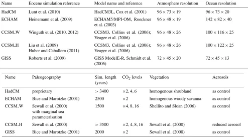
Fig. 1. SST proxy dataset, compiled for this study. Coloured symbols show the various median estimates from the literature, with various

asumptions about Mg/Ca of sewater,δ18_O

sw, and TEX86calibration. Error bars indicate the maximum and minimum range at each site

including temporal variability and calibration error. The filled black circles represent the mean SST at each site, averaged over the various assumptions. Larger symbols represent ‘background’ early Eocene state, smaller symbols represent the EECO. See Section 3.1 for more details.

Global mean SST [degrees C]

x1 x2 x4 x8 x16

CO2 relative to preindustrial 15

20 25 30

temperature

HadCM3L

HadCM3L ECHAM5

ECHAM5

CCSM3_W

CCSM3_W GISS

GISS

CCSM_H

CCSM_H HADISST

(a)

Global mean surface temperature [degrees C]

x1 x2 x4 x8 x16

5 10 15 20 25 30

temperature

HadCM3L

HadCM3L ECHAM5

ECHAM5

CCSM3_W

CCSM3_W GISS

GISS

CCSM_H

CCSM_H NCEP

(b)

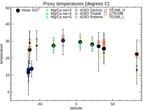
Fig. 2. Global annual mean (a) SST (hSSTi) and (b) continental 2m air temperature (hLATi), as a function of CO2for all simulations, and

for observational datasets. The simulations at×1 CO2are pre-industrial reference simulations.

Fig. 1. SST proxy dataset, compiled for this study. Coloured sym-bols show the various median estimates from the literature, with various assumptions about Mg/Ca of seawater,δ18Osw, and TEX86

calibration. Error bars indicate the maximum and minimum range at each site including temporal variability and calibration error. The filled black circles represent the mean SST at each site, aver-aged over the various assumptions. Larger symbols represent “back-ground” early Eocene state, smaller symbols represent the EECO. See Sect. 3.1 for more details.

non-analogue behaviour is very difficult to assess and we do not try to quantify this directly in our uncertainty anal-ysis. We do, however, attempt to quantify uncertainty asso-ciated with both paleotemperature calibrations and the es-timates of ancient seawater chemistry. This is achieved by (1) applying the standard error determined from the mod-ern calibration dataset to paleotemperature estimates; (2) the use of multiple alternate calibrations where there is ongo-ing debate about the most appropriate calibration or proxy method (GDGT paleothermometry) or where modern cal-ibrations vary with environmental conditions (oxygen iso-topes); and (3) applying multiple estimates (Mg/Ca) or dif-ferent estimation methodologies (oxygen isotopes) for sea-water chemistry. Where distinct proxies (GDGT paleother-mometry) or distinct parameters for seawater chemistry are used (Mg/Ca and oxygen isotopes), the derived temperature ranges are calculated separately at each site. This leads to the following sets of proxy data: TEXH₈₆, TEXL₈₆, 1/TEX86, oxygen isotope paleothermometry with modelled and latitu-dinal correctedδ18Oswestimates, and Mg/Ca paleothermom-etry with assumed Mg/Caswvalues of 3, 4 and 5 mol mol−1. Details of all these methods and calculations are described below, and illustrated in Fig. 1.

3.1.1 Oxygen isotopes

(6)

Orbulina universa, under both high and low light

con-ditions (their Eqs. 1 and 2). Together, these two equa-tions bracket most of the natural variability in planktic foraminifera temperature–δ18O space within modern plank-ton tow data (Bemis et al., 1998). Unlike the multiple GDGT paleotemperature equations, which seem to vary in their ac-curacy with geographical location or paleoenvironment, the two equations of Bemis et al. (1998) represent the natural variability at a single location (high/low light conditions). The derived SST estimates from these two equations are thus combined into a single range representing the potential en-vironmental variability at any location. The standard errors on Eq. (1) (low light) and 2 (high light) are±0.7 and 0.5◦C, respectively.

Three sets of temperature estimate are, however, plotted in Fig. 1 for each location with planktic foraminiferaδ18O data based on three estimates ofδ18Osw: the latitudinal cor-rection of Zachos et al. (2008) and the modelled mixed-layer

δ18Oswof Tindall et al. (2010) and of Roberts et al. (2011). The latitudinal correction is a first-order approximation of the effects of the global hydrological cycle on seawaterδ18Osw and is a widely used improvement on an “ice-free” globally uniform estimate ofδ18Osw. This empirical relationship does not, however, include zonal deviations from this general pat-tern. In the early Paleogene world, these zonal deviations are likely to have been significantly different to the modern due to the closure of the major Southern Ocean gateways and the resulting high-latitude isolation of the Atlantic and Pa-cific basins. The isotope-enabled versions of HadCM3L and GISS, however, reproduce both the expected latitudinal gra-dients inδ18Oswand an estimation of early Paleogene basin-to-basin zonal gradients (Tindall et al., 2010; Roberts et al., 2011). These modelledδ18Oswvalues, taken from modelled ocean depths of 50 m, are a potential refinement to early Pa-leogeneδ18Oswestimation and are included here to provide a more comprehensive assessment of the range of possible

δ18O SST estimates.

For the latitudinal correction, we assume a global average

δ18O composition of early Eocene seawater of−1_hto be consistent with the value used by Tindall et al. (2010). This is comparable to the−0.96_hused in a recent early Eocene pa-leotemperature inter-comparison (Hollis et al., 2012), and the value of−0.81_hused in Roberts et al. (2011). A SMOW to VPDB conversion of−0.27_hwas applied to all estimates of

δ18Osw. The maximum difference in paleotemperature esti-mates between the threeδ18Oswassumptions is for Seymour Island, where the median value using the modelledδ18Osw of Roberts et al. (2011) is 5.6◦_{C warmer than that using the} δ18Oswof Tindall et al. (2010).

For the Eurhomalea and Cucullaea bivalve δ18O data, we used the biogenic aragoniteδ18O–temperature calibration of Grossman and Ku (1986) as modified by Kobashi et al. (2003) with both the latitude-corrected and modelledδ18Osw noted above. We calculated the standard error on the Gross-man and Ku (1986) calibration, based on the original dataset

for biogenic aragonite, to be±1.4◦_{C. A SMOW to VPDB}

correction of−0.2_his already implicit within the Kobashi et al. (2003) form of this temperature equation.

3.1.2 Mg/Ca ratios of planktonic foraminifera

To estimate calcification temperature, we used the multi-species sediment trap calibration of Anand et al. (2003), which has a calibration standard deviation of ±1.13◦C. This paleotemperature estimation relies strongly upon the assumed value of the Mg/Ca ratio in early Eocene seawa-ter, which is still poorly constrained. Values in the range of 3–4 mol mol−1are typically used within paleoceanographic studies, and these produce tropical (Sexton et al., 2006) and mid-latitude (Creech et al., 2010) surface ocean tempera-tures that are broadly consistent with independent paleotem-perature estimates. Here, we separately calculate and plot (in Fig. 1) paleotemperature estimates based on three val-ues of seawater Mg/Ca across a wide range, namely 3, 4 and 5 mol mol−1. Distinguishing temperature estimates based on these three values allows for (1) a clear representation of the sensitivity of temperature to the assumed value of Mg/Casw, and (2) the future use of the most appropriate temperature range if/when more robust constraints on early Paleogene Mg/Caswbecome available.

For reference, an estimate of ∼3.5 mol mol−1 is ob-tained using the Lear et al. (2002) calibration for

Oridor-salis umbonatus, the paired foraminifera Mg/Ca value of

2.78 mol mol−1andδ18O-derived bottom water temperature of 12.4◦C they quote for∼49 Ma. A lower,∼3 mol mol−1 value is obtained by the same method but using the re-vised calibrations for O. umbonatus (Rathmann et al., 2004; Rathmann and Kuhnert, 2008). Higher values of ∼4 to 5 mol mol−1 are indicated by δ18O–Mg/Ca paleotempera-ture inter-comparisons with well-preserved early Eocene foraminifera (Sexton et al., 2006), whilst recent modelling of trace metal fluxes and assessments of the long-term ben-thic foraminifera δ18O–Mg/Ca record suggest values of ∼ 3 mol mol−1 or less (Cramer et al., 2011; Farkaˇs et al., 2007). These lower values are more consistent with estimates based on ridge flank hydrothermal carbonate veins, at around 2 mol mol−1(Coggon et al., 2010). There remains a pressing need to understand the causes of these discrepancies and es-tablish robust estimates of the Mg/Ca ratio of ancient seawa-ter (see discussion in Coggon et al., 2011).

3.1.3 TEX86

(7)

D. J. Lunt et al.: EoMIP 1723

Lunt et al: EoMIP

15

Proxy temperatures [degrees C]

-50 0 50

latitude 0

10 20 30 40 50

temperature

mean SST Mg/Ca sw=3 Mg/Ca sw=4 Mg/Ca sw=5

d18O Zachos d18O Tindall d18O Roberts

TEX86_H 1/TEX86 TEX86_L

Fig. 1. SST proxy dataset, compiled for this study. Coloured symbols show the various median estimates from the literature, with various

asumptions about Mg/Ca of sewater, δ18

Osw, and TEX86 calibration. Error bars indicate the maximum and minimum range at each site including temporal variability and calibration error. The filled black circles represent the mean SST at each site, averaged over the various assumptions. Larger symbols represent ‘background’ early Eocene state, smaller symbols represent the EECO. See Section 3.1 for more details.

Global mean SST [degrees C]

x1 x2 x4 x8 x16

20 25 30

temperature

HadCM3L

HadCM3L ECHAM5

ECHAM5

CCSM3_W

GISS

CCSM_H

CCSM_H HADISST

(a)

Global mean surface temperature [degrees C]

x1 x2 x4 x8 x16

5 10 15 20 25 30

temperature

HadCM3L

HadCM3L ECHAM5

ECHAM5

CCSM3_W

GISS

CCSM_H

CCSM_H NCEP

(b)

Fig. 2. Global annual mean (a) SST (hSSTi) and (b) continental 2m air temperature (hLATi), as a function of CO2for all simulations, and for observational datasets. The simulations at×1 CO2are pre-industrial reference simulations.

Fig. 2. Global annual mean (a) SST (hSSTi) and (b) continental 2 m air temperature (hLATi), as a function of CO₂for all simulations, and for observational datasets. The simulations at×1 CO2are pre-industrial reference simulations.

and a non-linear calibration of the original TEX86 index, “1/TEX86” (Liu et al., 2009), revised by Kim et al. (2010). TEXH₈₆and 1/TEX86 are based on the same underlying ratio of GDGTs – the original TEX86proxy – but differ in the form of their calibration equations (logarithmic versus reciprocal). The fundamentally different ratio of GDGT isomers within TEXL₈₆results in a proxy that can, in certain instances, pro-duce temperature trends contrary to TEXH₈₆ and 1/TEX86. It is, as yet, unclear which of these proxies is the most appro-priate for early Eocene paleotemperature estimation. There are indications that their suitability may vary with both the temperature range and paleoenvironment of GDGT forma-tion (Hollis et al., 2012).

For the purposes of this study, we separately calculate and plot (in Fig. 1) paleotemperatures at each site using all three measures: TEXH₈₆, TEXL₈₆and 1/TEX86. This illustrates the full range of temperature estimates produced by these GDGT-based proxies at a given location but also allows for a more refined use of this data as the behaviour of these prox-ies becomes better understood. The calculation of all three proxies at all sites may be considered by some to be an erroneous application of, for example, a “low temperature” proxy, TEXL₈₆, to the mid and low latitudes of a warm cli-mate state. We must stress that we do not intend to imply that all three are equally applicable at all sites. Rather, by showing all three proxies at all sites alongside other proxy temperature estimates, we hope to contribute to the ongoing discussion about the behaviour of GDGT proxies in deep-time paleoenvironments (Hollis et al., 2012).

Recent development of good practice suggests the exclu-sion of paleotemperature estimates from samples with a BIT index in excess of 0.3 (Kim et al., 2010). Although we ac-cept this as a recommendation, in the existing published data compiled here it would result in the exclusion of all early Eocene data from Tanzania and Hatchetigbee Bluff, which both have BIT indices in the range 0.3 to 0.5. We choose

to include this published data but note these higher BIT in-dices. In some cases, as for the early Eocene data from Tanza-nia, TEXL₈₆temperature estimates are clearly erroneous and are excluded. Due to the greater availability of data, sam-ples from the Arctic Ocean IODP Site M0004 with BIT in-dices>0.3 were excluded. The standard TEX86proxies dis-cussed above can be applied to this early Eocene Arctic data rather than the TEX86 proxy used through the PETM by Sluijs et al. (2006). The errors (◦C) on the GDGT-based prox-ies are±2.5 for TEXH₈₆ (GDGT index-2), ±4.0 for TEXL₈₆ (GDGT index-1) and±5.4 for 1/TEX86(Kim et al., 2010).

From the arrays of time-varying temperature estimates at each site, and for all assumptions of seawater composition and TEX86calibration, we calculated the median, maximum and minimum values from the time series as the basis for the model–data comparisons. There is an important caveat to this approach that relates to the effect of data quantity and strati-graphic range on the temperature envelopes plotted. Where there are reasonably extensive time series, natural tempo-ral variability can result in a larger envelope of temperature estimates than at sites where data is limited to a few spot samples. As a result, these envelopes should not be taken to solely represent uncertainty in paleotemperature estimation, but to also include a measure of the temporal variability at individual sites.

(8)

1724 D. J. Lunt et al.: EoMIP

16

Lunt et al: EoMIP

×2 ×4 ×6 ×8 ×16

HadCM

180W150W120W90W60W30W030E60E90E120E150E180E 90S 60S 30S 0 30N 60N 90N

HadCM3L - 2* CO2 anomaly

ECHAM

ECHAM5 - 2* CO2 anomaly

CCSM W

CCSM3_W - 4* CO2 anomaly

CCSM H

CCSM_H - 2* CO2 anomaly

GISS

GISS - 4* CO2 anomaly

-20.0 -16.0 -12.0 -8.0 -4.0 0.0 4.0 8.0 12.0 16.0 20.0

Temperature (Celsius)

Fig. 3. SST anomaly in the model simulations (SSTm

e −SSTpm), as a function of model and fractional CO2increase from pre-industrial.

Also shown for the proxies areSSTd

e−SSTpd.

×2 ×4 ×6 ×8 ×16

HadCM

ECHAM

CCSM W

CCSM H

GISS

-20.0 -16.0 -12.0 -8.0 -4.0 0.0 4.0 8.0 12.0 16.0 20.0

Fig. 4. Continental surface air temperature anomaly in the model simulations (LATem−GATpm), as a function of model and fractional CO2

increase from pre-industrial. Also shown for the proxies areLATd

e−GATpd.

Fig. 3. SST anomaly in the model simulations (SSTm_e −SSTm_p), as a function of model and fractional CO2increase from pre-industrial. Also

shown for the proxies are SSTd_e−SSTd_p.

others will be able to provide their own interpretation if nec-essary as data is re-interpreted.

3.2 Terrestrial dataset

For the terrestrial, we make use of the data compilation pre-sented in Huber and Caballero (2011). This is based largely on macrofloral assemblages, with mean annual temperatures being reconstructed primarily by leaf-margin analysis and/or CLAMP (physiognomic analysis of leaf fossils). Other prox-ies are also incorporated, such as isotopic estimates, organic geochemical indicators, and palynoflora. The error bars asso-ciated with each data point incorporate uncertainty in calibra-tion, topography, and dating. More information on the data themselves, and the estimates of uncertainty, can be found in Huber and Caballero (2011).

Both marine and terrestrial datasets are provided in the Supplement, and are plotted geographically in Figs. 3 and 4, and latitudinally in Figs. 5 and 7.

The SST plots have error bars which include the contri-butions from the two sources of uncertainty we have con-sidered, related to calibration and temporal trends. This ap-proach to the data aims to include a wide range of potential uncertainties in order to highlight both the regions of poten-tial model–data agreement, but more importantly where there appear to be genuine discrepancies that cannot realistically be explained by the uncertainties in the proxy temperature estimations.

4 Results and model–data comparison

In this section, we present results from the EoMIP model ensemble (early Eocene simulations and pre-industrial con-trols), as described in Sect. 2, and compare them with the data described in Sect. 3. The reasons for the different model results are explored in more detail in Sect. 5.

It is useful at this stage to define some nomenclature. To represent the distribution of temperature, we write SST for sea surface temperature (only defined over ocean), or LAT for land near-surface (∼1.5 m) air temperature (only defined over continents), or GAT for near-surface air temperature (defined globally), or GST for surface temperature (defined globally), or justT for a generic temperature. Global means are denoted by angled brackets, so that, for example, the global mean sea surface temperature ishSSTi. Zonal means are denoted by overbars, so that the zonal mean sea surface temperature is SST. In the case of model output, ensem-ble means are denoted by square brackets, such as [LAT]. Eocene quantities are given a subscript e, and present/pre-industrial (i.e. modern) quantities are given a subscript p. Model values are given a superscript m, and proxy or ob-served data are given a superscript d. Because the modern observed data has global coverage (albeit interpolated, or assimilated with models in some regions), but the Eocene proxy data is sparse, the modern observed global or zonal meanshT_pdiandTd

(9)

D. J. Lunt et al.: EoMIP 1725

16

Lunt et al: EoMIP

×2 ×4 ×6 ×8 ×16

HadCM

ECHAM

CCSM W

CCSM H

GISS

-20.0 -16.0 -12.0 -8.0 -4.0 0.0 4.0 8.0 12.0 16.0 20.0

Fig. 3. SST anomaly in the model simulations (SSTm

e −SSTpm), as a function of model and fractional CO2increase from pre-industrial.

Also shown for the proxies areSSTd

e−SSTpd.

×2 ×4 ×6 ×8 ×16

HadCM

ECHAM

CCSM W

CCSM H

GISS

-20.0 -16.0 -12.0 -8.0 -4.0 0.0 4.0 8.0 12.0 16.0 20.0

Fig. 4. Continental surface air temperature anomaly in the model simulations (LATm

e −GATpm), as a function of model and fractional CO2

increase from pre-industrial. Also shown for the proxies areLATd

e−GATpd.

Fig. 4. Continental surface air temperature anomaly in the model simulations (LATm_e −GATm_p), as a function of model and fractional CO2

increase from pre-industrial. Also shown for the proxies are LATd_e−GATd_p.

Table 2. Global mean temperatures and model mean error scores for each simulation. Scores are calculated based on the SST (σsst) and

land surface air temperature (σlat) data. Definitions of the scores are

given in Eqs. (1) and (2). Rows in bold indicate the best (i.e. lowest

σ) CO2level for each model.

Model CO2 hSSTi hLATi hGSTi σsst(◦C) σlat(◦C)

HadCM 2× 21.45 11.71 18.54 8.8 15.5 4× 24.19 16.20 21.95 6.0 11.4

6× 26.25 19.80 24.56 3.9 7.7

ECHAM 2× 24.65 20.59 24.03 5.8 9.7

CCSM W 4× 22.24 16.26 20.95 6.7 10.3 8× 24.45 19.57 23.59 4.0 7.2

16× 27.14 23.16 26.46 0.9 3.7

CCSM H 2× 22.15 15.71 21.12 8.6 11.5 4× 23.94 18.41 23.17 6.6 8.5 8× 26.43 21.66 25.79 3.6 5.1

16× 29.75 26.30 29.47 0.0 0.4

GISS 4× 26.43 21.97 23.25 3.8 6.9

4.1 Inter-model comparison

Figure 2 shows the global annual mean sea surface tem-perature,hSSTi, and global annual mean near-surface land air temperature, hLATi, from all the GCM simulations in the EoMIP ensemble, and for modern observations; the Eocene values are also given in Table 2. The observed mod-ern datasets are HadISST for SSTs (pre-industrial; 1850– 1890) and NCEP (Kalnay et al., 1996) for near-surface air

temperatures (present; 1981–2010). For any given CO2level, there is a wide range of modelled Eocene global mean values; for example, at 560 ppmv, there is a 8.9◦C range inhLATm_ei and a 3.2◦C range in hSSTm_ei. This range is larger than the range of simulated modern global means, which them-selves agree well with the observed modern global means. The spread in Eocene results is due to (a) differences in the way the Eocene boundary conditions have been imple-mented in different models, and (b) different climate sen-sitivities in the different models. These differences are ex-plored in Sect. 5. The clustering of the pre-industrial results is likely a result of tuning of the pre-industrial simulations to best match observations. For those models with more than one Eocene simulation, the Eocene climate sensitivity (1

(10)

1726 D. J. Lunt et al.: EoMIP

Lunt et al: EoMIP 17

Proxy/model temperatures [degrees C] - HadCM3L

-50 0 50 latitude 0

10 20 30 40 50

temperature

2* CO2 4* CO2 6* CO2 1* CO2 mean SST

(a)

Proxy/model temperatures [degrees C] - ECHAM5

-50 0 50 latitude 0

10 20 30 40 50

temperature

2* CO2 1* CO2 mean SST

(b)

Proxy/model temperatures [degrees C] - CCSM3_W

-50 0 50 latitude 0

10 20 30 40 50

temperature

(c)

Proxy/model temperatures [degrees C] - CCSM_H

-50 0 50 latitude 0

10 20 30 40 50

temperature

2* CO2 4* CO2 8* CO2 16* CO2 1* CO2 mean SST

(d)

Proxy/model temperatures [degrees C] - GISS

-50 0 50 latitude 0

10 20 30 40 50

temperature

(e)

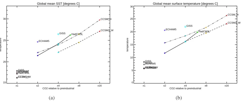
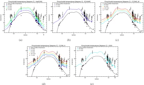
Fig. 5. Comparison of modelled SST with proxy-derived temperatures, SST vs. latitude. The simulations at×1 CO2are pre-industrial reference simulations. For the model results, the continous lines represent the zonal mean, and the open symbols represent the modelled temperature at the same location (longitude,latitude) as the proxy data. For the proxy data, the filled symbols represent the mean proxy temperature, and the error bars represent the range. The smaller fille d symbols are EECO temperatures. See Section 3 and Supplementary Information for more details of the range calculations.

-50 0 50

latitude 0

10 20 30 40 50

temperature

2* CO2 4* CO2 6* CO2 mean SST

(a)

-50 0 50

latitude 0

10 20 30 40 50

temperature

(b)

Fig. 6. As Figure 5a and d, but the HadCM and CCSM H modelled zonal mean represents the warm month mean SST, as opposed to annual mean.

Fig. 5. Comparison of modelled SST with proxy-derived temperatures, SST vs. latitude. The simulations at×1 CO2are pre-industrial

reference simulations. For the model results, the continous lines represent the zonal mean, and the open symbols represent the modelled temperature at the same location (longitude, latitude) as the proxy data. For the proxy data, the filled symbols represent the mean proxy temperature, and the error bars represent the range. The smaller filled symbols are EECO temperatures. See Sect. 3 and the Supplement for more details on the range calculations.

×1 CO2 (not shown). Comparison of that simulation with its pre-industrial control shows that changing the non-CO2 boundary conditions to those of the Eocene (i.e. topographic, bathymetric, vegetation, and solar constant changes) results in a 1.8◦_{C increase in global mean surface air temperature,}

by comparison with a 3.3◦C increase for a CO2 doubling from×1 to ×2 under Eocene conditions. At a given CO2 level, the CCSM W and CCSM H models give quite differ-ent global means. This difference in mean Eocene climate state between the two similar models is mostly due to dif-ferences in the assumed Eocene atmospheric aerosol load-ing; CCSM W includes modern aerosols, whereas CCSM H includes no aerosol loading (see Sect. 2 and Table 1). Both these models share the same pre-industrial simulation. For all models, thehLATiandhSSTimeans share similar character-istics, albeit withhSSTivarying over a smaller temperature range.

Figure 3 shows the simulated annual mean SST anomaly from each model and for the proxy reconstructions. A sim-ple anomaly SSTe−SSTp would not be particularly infor-mative because many regions would be undefined due to the difference in continental positions between the Eocene and present. Instead, we show SSTe−SSTp, which is only undefined over Eocene continental regions and latitudes at which there is no ocean in the modern. The figures show that some features of temperature change are simulated con-sistently across models, such as the greatest ocean warming occurring in the mid latitudes. This mid-latitude maximum is due to reduced SST warming in the high latitudes due to the presence of seasonal sea ice anchoring the temperatures

close to 0◦C combined with reduced warming in the tropics due to a lack of snow and sea ice albedo feedbacks. How-ever, other patterns are not consistent. For example, GISS at ×4 and HADCM at ×6 have similar values of hSSTi relative to their controls (8.6 and 9.0◦_{C, respectively), but}

the warming in GISS is greatest in the northeast Pacific and the Southern Ocean, and the warming in HADCM is great-est in the North Atlantic and wgreat-est of Australia. Similarly, ECHAM at×2 and CCSM H at×4 have similar global mean SST anomalies (7.2 and 7.6◦C, respectively), but the greatest Northern Hemisphere warming is in the Atlantic for ECHAM and in the Pacific for CCSM H. The two CCSM models ex-hibit similar patterns of warming, correcting for their offset in absolute Eocene temperature – i.e. the patterns of warming in CCSM H at×8 are similar to those in CCSM W at×16 (with anomalies of 10.1 and 10.8◦C, respectively).

(11)

D. J. Lunt et al.: EoMIP 1727

Lunt et al: EoMIP

17

-50 0 50 latitude 0

10 20 30 40 50

temperature

(a)

-50 0 50 latitude 0

10 20 30 40 50

temperature

(b)

-50 0 50 latitude 0

10 20 30 40 50

temperature

(c)

-50 0 50 latitude 0

10 20 30 40 50

temperature

2* CO2 4* CO2 8* CO2 16* CO2 1* CO2 mean SST

(d)

-50 0 50 latitude 0

10 20 30 40 50

temperature

(e)

Fig. 5. Comparison of modelled SST with proxy-derived temperatures, SST vs. latitude. The simulations at×1 CO2 are pre-industrial

reference simulations. For the model results, the continous lines represent the zonal mean, and the open symbols represent the modelled temperature at the same location (longitude,latitude) as the proxy data. For the proxy data, the filled symbols represent the mean proxy temperature, and the error bars represent the range. The smaller fille d symbols are EECO temperatures. See Section 3 and Supplementary Information for more details of the range calculations.

-50 0 50

latitude 0

10 20 30 40 50

temperature

2* CO2 4* CO2 6* CO2 mean SST

(a)

-50 0 50

latitude 0

10 20 30 40 50

temperature

(b)

Fig. 6. As Figure 5a and d, but the HadCM and CCSM H modelled zonal mean represents the warm month mean SST, as opposed to annual

mean.

Fig. 6. As Fig. 5a and d, but the HadCM and CCSM H modelled zonal mean represents the warm month mean SST as opposed to annual mean.

×2 have similar values of hLATi relative to their controls (8.5 and 7.3◦C, respectively), but GISS has a substantially greater warming over Southeast Asia. These differences can-not be explained solely by differences in topography – the GISS and ECHAM models both use the Eocene topography of Bice and Marotzke (2001).

4.2 Model–data comparison

Figure 5 shows a zonal SST model–data comparison for each model. The longitudinal locations of the SST data can be seen in Fig. 3. Each model is capable of simulating Eocene SSTs which are within the uncertainty estimates of the majority of the data points. The data points which lie furthest from the model simulations are the ACEX TEX86 Arctic SST estimate (Sluijs et al., 2006), and theδ18O and TEX86 estimates from the southwest Pacific (Bijl et al., 2009). The Arctic temperature reconstructions have uncer-tainty estimates which mean that at high CO2, the CCSM H (×8–16) and CCSM W (×16) model simulations are just within agreement. At this CO2 level, these models are also consistent with most of the tropical temperature estimates. From Fig. 2a, it is likely that other models could also obtain similarly high Arctic temperatures if they were run at suf-ficiently high CO2or low aerosol forcing. Also, given that some of these models (e.g. HadCM) have a higher climate sensitivity than CCSM H, this model–data consistency could be potentially obtained at a lower CO2than in CCSM.

TEX86 is a relatively new proxy, which, as discussed in Sect. 3, is currently undergoing a process of rapid develop-ment. In this context, it has been suggested that the proxy could be recording the paleotemperature anomaly of the bloom season of the marine archaeota as opposed to a true annual mean. If this is the case, then it is likely that a more appropriate comparison is with the modelled summer tem-perature. This is illustrated in Fig. 6, for the HadCM and

CCSM H models. In this case, the modelled warm month mean temperature is within the uncertainty range of the Arc-tic TEX86temperatures for both models.

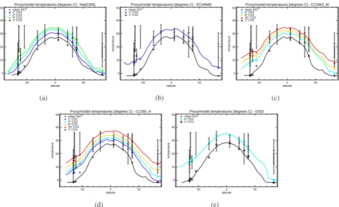
Figure 7 shows the terrestrial temperature model–data comparison for each model. Those models which have been run at high CO2(both CCSM models), show good agreement with the data across all latitudes. The other models do not simulate such high temperatures, but, as with SST, it does appear that if they had been run at higher CO2, the model– data agreement would have been better. The HadCM model appears to be somewhat of an outlier in the Northern Hemi-sphere high latitudes, as it shows less polar amplification than the other models (see Sect. 4.3), an effect also seen in SST.

A quantitative indication of the model–data comparison for each simulation cannot currently be used to rank the models themselves, because the actual CO2 forcing is not well constrained by data. However, it could give an indication of the range of CO2concentrations which are most consistent with the data. Given the sparseness of the SST and terrestrial data, any score should be treated with some caution. This is confounded by the uneven spread of the data; for example, there is a relatively high concentration of terrestrial data in North America. There are also issues associated with the dif-ferent land–sea masks in the difdif-ferent models, which mean that the number of proxy data locations at which there are de-fined modelled values differs between the models. Therefore, we generate a simple mean error score for each simulation,

σ, for both SST (σsst) and land air temperature (σlat) by av-eraging the error in temperature anomaly at the location of each ofN data points:

σsst=

1

N

X

(SSTm_e −SSTm_p −SSTd_e+SSTd_p), (1)

σlat=

1

N

X

(12)

1728 D. J. Lunt et al.: EoMIP

18

Lunt et al: EoMIP

-50 0 50

latitude -20

0 20 40

temperature

2* CO2 4* CO2 6* CO2 1* CO2

proxy surface temperature

(a)

-50 0 50

latitude -20

0 20 40

temperature

2* CO2 1* CO2

(b)

-50 0 50

latitude -20

0 20 40

temperature

4* CO2 8* CO2 16* CO2 1* CO2

(c)

-50 0 50

latitude -20

0 20 40

temperature

2* CO2 4* CO2 8* CO2 16* CO2 1* CO2

(d)

-50 0 50

latitude -20

0 20 40

temperature

4* CO2 1* CO2

(e)

Fig. 7. Comparison of modelled SAT with proxy-derived temperatures, SAT vs. latitude. The simulations at

×

1 CO

2

are pre-industrial

ref-erence simulations. For the model results, the continous lines represent the zonal mean, and the symbols represent the modelled temperature

at the same location (longitude,latitude) as the proxy data. For the proxy data, the symbols represent the proxy temperature, and the error

bars represent the range, as given by Huber and Caballero (2011).

Proxy/model temperatures [degrees C]

-50 0 50

latitude 0

10 20 30 40 50

temperature

(a)

-50 0 50

latitude 0

10 20 30 40 50

temperature

(b)

Fig. 8. Zonal ensemble mean model (middle thick black line), and data, presented as an anomaly relative to present/pre-industrial. Outer

thick black lines indicate

±

2 standard deviations in the models. Coloured lines represent each individual model simulation in the ensemble,

with the colour indicating CO

2

level as in Figures 5 and 7. (a)

[

SST

e

−

SST

p

]

. (b)

[

LAT

e

−

GAT

p

]

. For this Figure, the ensemble consists

of the best simulation from each model, as highlighted in bold in Table 2. Descriptions of the proxy error bars are given in the captions to

Fig. 7. Comparison of modelled SAT with proxy-derived temperatures, SAT vs. latitude. The simulations at×1 CO2are pre-industrial

refer-ence simulations. For the model results, the continous lines represent the zonal mean, and the symbols represent the modelled temperature at the same location (longitude, latitude) as the proxy data. For the proxy data, the symbols represent the proxy temperature, and the error bars represent the range, as given by Huber and Caballero (2011).

but proceed with caution, being mindful that there is a con-siderable uncertainty in the score itself. Values ofσ for each model simulation are given in Table 2. For each model, the best results are obtained for the highest CO2level which was simulated (a result which also applies if an RMS score is used in place of a mean error score). The CCSM H model at 16×CO2has the best (i.e. lowest absolute) values ofσ. However, as noted before, it appears that other models would also obtain goodσ scores if they had been run at sufficiently high CO2. A “best-case” multi-model ensemble can be cre-ated by averaging the simulations from each model which have the lowest values of σ (it turns out that those mod-els with the bestσlat also have the bestσsst). These are the models highlighted in bold in Table 2. The model–data com-parison for this multi-model ensemble is shown in Figs. 8 and 9. The 2 standard-deviation width of the “best-case” ensemble overlaps the uncertainty estimates of every terres-trial and ocean proxy data point. However, the high latitude southwest Pacific SST estimates are right at the boundary of consistency. The terrestrial data shows very good agreement with the model ensemble, and both data and models show a similar degree of polar amplification (see Sect. 4.3).

By regressing the CO2 levels andσ values in Table 2, it is possible (for those models with more than one Eocene

simulation) to provide a first-order estimate of the CO2level, for each model, which could give the best agreement with the proxy estimates. For HadCM, CCSM H, and CCSM W, usingσsstthis is 2600 ppmv, 4300 ppmv, and 4900 ppmv, re-spectively, and usingσlatthis is 2800 ppmv, 4500 ppmv, and 6300 ppmv, respectively. These estimates come with many caveats, not least that the uneven and sparse data spread means that the absolute minimum mean error,σ, is not nec-essarily a good indicator of the correct global mean tempera-ture. However, they do indicate the magnitude of the range of CO2values that could be considered consistent with model results. These values are significantly higher than those pre-sented for this time period in the compilation of Beerling and Royer (2011).

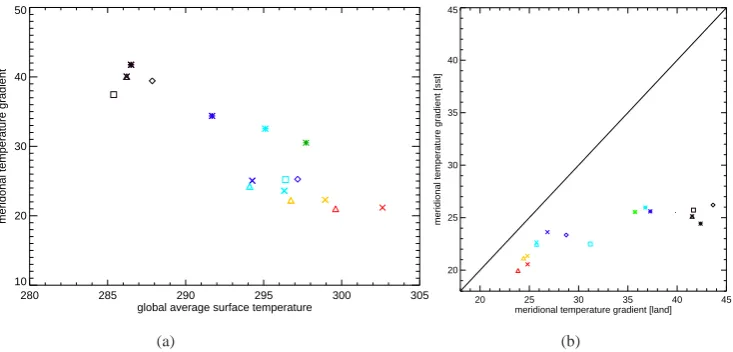
4.3 Meridional gradients and polar amplification

The changes in meridional temperature gradient are sum-marised in Fig. 10, which shows the surface temperature dif-ference between the low latitudes (|φ|<30◦) and the high latitudes (|φ|>60◦) as a function of global mean temper-ature, and how this is partitioned between land and ocean warming (Fig. 10b,φis latitude in degrees). All the Eocene simulations have a reduced meridional surface temperature

(13)

D. J. Lunt et al.: EoMIP 1729

18

Lunt et al: EoMIP

-50 0 50 latitude -20

0 20 40

temperature

2* CO2 4* CO2 6* CO2 1* CO2 proxy surface temperature

(a)

-50 0 50 latitude -20

0 20 40

temperature

2* CO2 1* CO2 proxy surface temperature

(b)

-50 0 50 latitude -20

0 20 40

temperature

4* CO2 8* CO2 16* CO2 1* CO2 proxy surface temperature

(c)

-50 0 50 latitude -20

0 20 40

temperature

2* CO2 4* CO2 8* CO2 16* CO2 1* CO2 proxy surface temperature

(d)

-50 0 50 latitude -20

0 20 40

temperature

4* CO2 1* CO2 proxy surface temperature

(e)

Fig. 7. Comparison of modelled SAT with proxy-derived temperatures, SAT vs. latitude. The simulations at×1 CO2are pre-industrial

ref-erence simulations. For the model results, the continous lines represent the zonal mean, and the symbols represent the modelled temperature at the same location (longitude,latitude) as the proxy data. For the proxy data, the symbols represent the proxy temperature, and the error bars represent the range, as given by Huber and Caballero (2011).

-50 0 50

latitude 0

10 20 30 40 50

temperature

(a)

-50 0 50

latitude 0

10 20 30 40 50

temperature

(b)

Fig. 8. Zonal ensemble mean model (middle thick black line), and data, presented as an anomaly relative to present/pre-industrial. Outer

thick black lines indicate±2 standard deviations in the models. Coloured lines represent each individual model simulation in the ensemble, with the colour indicating CO2level as in Figures 5 and 7. (a)[SSTe−SSTp]. (b)[LATe−GATp]. For this Figure, the ensemble consists

of the best simulation from each model, as highlighted in bold in Table 2. Descriptions of the proxy error bars are given in the captions to Figures 5 and 7.

Fig. 8. Zonal ensemble mean model (middle thick black line), and data, presented as an anomaly relative to present/pre-industrial. Outer thick black lines indicate±2 standard deviations in the models. Coloured lines represent each individual model simulation in the ensemble, with the colour indicating CO2level as in Figs. 5 and 7. (a)[SSTe−SSTp]. (b)[LATe−GATp]. For this figure, the ensemble consists of the

best simulation from each model, as highlighted in bold in Table 2. Descriptions of the proxy error bars are given in the captions to Figs. 5 and 7.

Lunt et al: EoMIP

19

180W 150W 120W 90W 60W 30W 0 30E 60E 90E 120E 150E 180E 90S

60S 30S 0 30N 60N 90N

Eocene_ensemble

-20.0 -16.0 -12.0 -8.0 -4.0 0.0 4.0 8.0 12.0 16.0 20.0 Temperature (Celsius)

180W 150W 120W 90W 60W 30W 0 30E 60E 90E 120E 150E 180E 90S

60S 30S 0 30N 60N 90N

Eocene_ensemble

(a)

180W 150W 120W 90W 60W 30W 0 30E 60E 90E 120E 150E 180E 90S

60S 30S 0 30N 60N 90N

Eocene_ensemble

180W 150W 120W 90W 60W 30W 0 30E 60E 90E 120E 150E 180E 90S

60S 30S 0 30N 60N 90N

Eocene_ensemble

(b)

Fig. 9. Ensemble mean modelled Eocene warming, presented as an anomaly relative to present/pre-industrial. (a) [SSTe−SSTp]. (b)

[LATe−GATp]. The ensmble consists of the best simulation from each model, as highlighted in bold in Table 2.

280 285 290 295 300 305

global average surface temperature 10

20 30 40 50

meridonal temperature gradient

(a)

20 25 30 35 40 45

meridional temperature gradient [land] 20

25 30 35 40 45

meridional temperature gradient [sst]

(b)

Fig. 10. (a) Meridional surface temperature gradientGST|φ|>60−GST|φ|<30, where|φ|is the absolute value of the latitude in degrees, as Fig. 9. Ensemble mean modelled Eocene warming, presented as an anomaly relative to present/pre-industrial. (a)[SSTe−SSTp]. (b)[LATe−

GATp]. The ensemble consists of the best simulation from each model, as highlighted in bold in Table 2.

gradient compared with the pre-industrial, and the gradi-ent reduces further as CO2 increases, i.e. polar amplifica-tion increases (Fig. 10a). However, there is a high degree of inter-model variability in the absolute Eocene gradient, with HadCM appearing to be an outlier with a relatively high Eocene gradient. There is some indication that the models are trending towards a minimum gradient of about 20◦C. This, along with our energy flux analysis (see Sect. 5), supports previous work (Huber et al., 2003) that implied that merid-ional temperature gradients of the order 20◦C were physi-cally realistic, even without large changes to meridional heat transport. Compared with pre-industrial, the meridional sur-face temperature gradient reduces more on land than over ocean (Fig. 10b). For HadCM, this applies also to the Eocene simulations as CO2 increases. However, for the two CCSM

models, the meridional temperature gradient is reduced by a similar amount over land and ocean as a function of CO2, with some indication, at maximum (×16) CO2, that the SST gradient starts reducing more over ocean than over land. This implies that when considering changes relative to the mod-ern, it is possible to have substantially different temperature changes over land compared with over ocean at the same lat-itude. This is also clear from comparing Fig. 3 with Fig. 4, and shows the importance of differentiating terrestrial and oceanic signals when considering the consistency between different proxy data, and between data and models.

(14)