www.earth-syst-dynam.net/3/49/2012/ doi:10.5194/esd-3-49-2012
© Author(s) 2012. CC Attribution 3.0 License.
Earth System
Dynamics
Comparison of physically- and economically-based
CO
2
-equivalences for methane
O. Boucher
Laboratoire de M´et´eorologie Dynamique, Institut Pierre Simon Laplace, CNRS – UMR8539, Universit´e Pierre et Marie Curie, 4 place Jussieu, 75252 Paris Cedex 05, France
Correspondence to: O. Boucher ([email protected])
Received: 4 January 2012 – Published in Earth Syst. Dynam. Discuss.: 13 January 2012 Revised: 25 April 2012 – Accepted: 11 May 2012 – Published: 22 May 2012
Abstract. There is a controversy on the role methane (and other short-lived species) should play in climate mitiga-tion policies, and there is no consensus on what an optimal methane CO2-equivalence should be. We revisit this question
by discussing some aspects of physically-based (i.e. global-warming potential or GWP and global temperature change potential or GTP) and socio-economically-based climate metrics. To this effect we use a simplified global damage potential (GDP) that was introduced by earlier authors and investigate the uncertainties in the methane CO2-equivalence
that arise from physical and socio-economic factors. The me-dian value of the methane GDP comes out very close to the widely used methane 100-yr GWP because of various com-pensating effects. However, there is a large spread in possible methane CO2-equivalences from this metric (1–99 %
inter-val: 10.0–42.5; 5–95 % interinter-val: 12.5–38.0) that is essentially due to the choice in some socio-economic parameters (i.e. the damage cost function and the discount rate). The main fac-tor differentiating the methane 100-yr GTP from the methane 100-yr GWP and the GDP is the fact that the former metric is an end-point metric, whereas the latter are cumulative met-rics. There is some rationale for an increase in the methane CO2-equivalence in the future as global warming unfolds,
as implied by a convex damage function in the case of the GDP metric. We also show that a methane CO2-equivalence
based on a pulse emission is sufficient to inform multi-year climate policies and emissions reductions, as long as there is enough visibility on CO2prices and CO2-equivalences for
the stakeholders.
1 Introduction
Methane (CH4) is one of the greenhouse gases that are
present in trace concentrations in the Earth’s atmosphere. Its concentration has increased steadily since the beginning of the industrial era, from 715 ppbv in 1750 to 1774 ppbv in 2005 (Forster et al., 2007). The radiative efficiency of methane is larger than that of carbon dioxide (CO2), so
that methane is the second most important anthropogenic greenhouse gas, although its concentration only increased by about 1 ppmv. Methane is directly responsible for a ra-diative forcing (RF) of 0.48 W m−2in 2005, compared to a RF of 1.66 W m−2for carbon dioxide (Forster et al., 2007). Methane emissions also contribute an indirect RF through changes in tropospheric ozone, stratospheric water vapour and CO2concentrations.
It has been shown that a multi-gas mitigation strategy is cheaper than a CO2-only mitigation policy (e.g. van Vuuren
et al., 2006), because it offers more flexibility in emission re-ductions across industrial sectors, space and time. A multi-gas approach, such as the Kyoto protocol, requires defin-ing CO2-equivalences for the non-CO2 gases. Such CO2
to account for the oxidation of methane into CO2.
Alterna-tively, methane emissions from fossil reservoirs should be reported both as CH4and CO2emissions in national
invento-ries (Gillenwater, 2008), which is not the case at the moment (IPCC, 2006).
There are different views held among climate change stakeholders regarding the importance of methane emission reductions in mitigation policies (Boucher, 2010). Some ar-gue that methane anthropogenic emissions should be curbed now and to a large extent, because, given the short atmo-spheric lifetime of methane, this will lead to a rapid de-crease in RF and consequently to a rapid slowdown of cli-mate change. The same argument can be applied to other short-lived species, such as precursors to tropospheric ozone – another greenhouse gas – or black carbon – an aerosol species that contribute to global warming. This view was ini-tially promoted by Hansen et al. (2000) and is held by some scientists and environmental groups. A more ambitious sion reduction target for methane does not mean that emis-sions of carbon dioxide should not be reduced, but overall this line of thinking argues for a larger CO2-equivalence for
methane.
Others argue that the emphasis should currently be on CO2 emission reductions, because a significant fraction of
the CO2emitted today will stay in the atmosphere for as long
as centuries. Given that mitigation of climate change bears a cost for society, and that only a fraction of public wealth can be spent on climate change, it is further argued that it is more important to start reducing CO2 emissions now or to invest
in research and development in order to decrease CO2
sions more cheaply and more quickly later on. Methane emis-sion reductions can come in a few decades time, because the atmospheric concentration of methane will respond quickly when these occur. This line of thinking argues for a smaller CO2-equivalence for methane.
It is unfortunate however that the public debate on the methane CO2-equivalence is often largely disconnected from
physical and socio-economic considerations. Ideally, the methane CO2-equivalence should rely on a suitable climate
metric that seeks to compare the climate effects of differ-ent greenhouse gases. IPCC (2009) reviewed existing climate metrics and made the point that a climate metric is a function of the climate policy. There are essentially two classes of climate metrics: physically-based and socio-economically-based metrics.
Physically-based metrics compare the relative effects of forcing agents in terms of a physical quantity of the cli-mate system, such as the cumulative radiative forcing in the case of the GWP or the global mean surface temperature change in the case of the global temperature change potential (GTP, Shine et al., 2005, 2007). Socio-economically-based metrics compare the relative costs of forcing agents on the climate system. This can be done in a cost-benefit fram-ing that seeks to optimise the emission and concentration pathways of CO2and non-CO2forcing agents. In that case
the CO2-equivalence is defined as the ratio of the marginal
costs of abatement of the non-CO2gas with that of CO2and
is equal to the ratio of cumulative damages caused by unit emissions of the two gases (Kandlikar, 1996). Such a CO2
-equivalence varies in time as we progress along some eco-nomic optimum, which may also evolve over time as more knowledge becomes available. This approach was used by Manne and Richels (2001), who showed that for a climate target of 2◦C, the methane CO2-equivalence should increase
from 5–10 at the beginning of the 21st century to 40–50 at the end of the 21st century. However, when they introduced a further climate target to limit the rate of global warming to 0.2◦C per decade, Manne and Richels (2001) found that the methane CO2-equivalence takes a value in the range 20–30
during all of the 21st century. The cost-effective temperature change potential introduced by Johansson (2012) can be seen as a simplified version of this metric that reduces to the GTP before the climate target is reached but can be extended be-yond that. Shine et al. (2007) introduced a time horizon that is a function of the proximity to a target year, which makes the physical metric dynamic, and reproduces qualitatively the results of Manne and Richels (2001).
A socio-economically-based climate metric can also be framed as the ratio of the climate damages caused by unit emissions of the two gases along some a priori concentration or temperature pathway (Kandlikar, 1996). This is the con-cept of the economic damage index introduced by Hammitt et al. (1996), which we refer to here as a global damage po-tential (GDP). Tol et al. (2008) showed how different existing climate metrics could be reconciled under a restrictive set of assumptions.
The simplicity of the GWP, with the lack of robustness of other metrics, has led to its adoption as the metric for CO2
-equivalence in the Kyoto protocol, with the consequence of casting the concept in stone (Shine, 2009). Earlier alternative metrics such as those of Hammitt et al. (1996) and Kandlikar (1996) have somewhat become forgotten, while there is still active literature on GWP (e.g. Boucher et al., 2009; Reisinger et al., 2010; Gillett and Matthews, 2010; Reisinger et al., 2011). Only the concept of GTP has recently been gaining some momentum as an alternative (IPCC, 2009; Fuglestvedt et al., 2010).
In the real world, CO2-equivalences are used in a
num-ber of different contexts. In the United Nations Framework Convention on Climate Change (UNFCCC) and the Ky-oto prKy-otocol, the GWP with a time horizon of 100 yr is used to estimate the total (i.e. CO2-equivalent) greenhouse
gas emissions for each country, and emission targets are also formulated in terms of CO2-equivalent emissions. A
CO2-equivalence is also required by policymakers to guide
the breakdown of their emission reduction target between gases within their own countries. Where a multi-gas emis-sion trading scheme (ETS) exists, a CO2-equivalence is
CO2-equivalences when deciding between different
invest-ments aimed at cutting emissions. A legitimate question is whether the different usages of CO2-equivalences
identi-fied above call for the same or different metrics. A related question is how to value pulse (i.e. one-off) and sustained (i.e. perennial) emission reductions of greenhouse gases such as methane.
The objectives of this study are threefold:
1. to revisit the concept of GDP and its sensitivity to input variables,
2. to compare the GWP and GTP with a simplified GDP in terms of their uncertainties and future time evolution, 3. and to discuss whether different usages of CO2
-equivalences require one or more climate metrics, e.g. in the context of perennial emission reduction.
We define the different metrics in Sect. 2, compare them in Sect. 3, and finally discuss the use of CO2-equivalences in
Sect. 4.
2 Definition of climate metrics used in this study
2.1 Global warming potential
The methane GWP is defined as the ratio of the methane and CO2absolute GWP at a starting timetin the future:
GWPCH4(t )=
AGWPCH4(t )
AGWPCO2(t ) =
TH R
0
RFCH4(t +t 0)dt0
TH R
0
RFCO2(t +t0)dt0
(1)
where RF(t+t0) is the radiative forcing at time t+t0 of a pulse emission of 1 kg occurring at timetand TH is an arbi-trary time horizon. The time horizon is usually set to 100 yr, but other values can be used, or it can decrease in time. 2.2 Global temperature change potential
The methane GTP is defined as the ratio of the absolute GTP of methane and CO2for a starting timetin the future:
GTPCH4(t )=
AGTPCH4(t )
AGTPCO2(t )
= δTCH4(t +TH) δTCO2(t +TH)
(2) where δT (t+ TH) is the global mean surface temperature (GMST) at a time horizon TH, caused by a pulse emission of 1 kg of either CO2or CH4occurring at timet.
2.3 Global damage potential
We define a simplified GDP for methane as the ratio of the absolute GDP of CH4and CO2for a pulse emission at a
start-ing timetin the future:
GDPCH4(t )=
AGDPCH4(t )
AGDPCO2(t )
= ∞ R
t0=0
[D(1T (t+t0)+δT
CH4(t+t
0))−D(1T (t+t0))]/(1+ρ)t0
dt0
∞ R
t0=0
[D(1T (t+t0)+δT
CO2(t+t0))−D(1T (t+t0))]/(1+ρ)t
0
dt0
(3)
where D is a damage cost function, δTCH4(t+t
0) and
δTCO2(t+t
0)are the GMST changes at timet+t0due to pulse
emissions of 1 kg of CH4and CO2at time t superimposed
on a trajectory of GMST change1T (t+t0), andρ is a dis-count rate, which is discussed in the next section. Integrating climate damage over time is justified, because climate im-pacts either depend on the repetitiveness of climate extremes (e.g. droughts, floods, ...) or on the cumulative amount of warming (e.g. sea level rise, glacier melting, sea-ice melting, permafrost thawing). Moreover, time-integrated damage un-derlies most cost-benefit analysis of climate change.
It should be noted that, if we omit potential future changes in radiative efficiencies and residence times, AGDPCH4,
AGDPCO2 and GDPCH4 are independent oft, if1T (t )≡0
or ifDis a linear function of1T, but are a function of the baseline yeartotherwise. In a warming climate (i.e.1T in-creases with time), GDPCH4increases with the baseline year,
ifDis a convex function of1T, which is usually the case. 2.4 Parametrising and sampling parametric
uncertainties
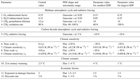
Our list of variable parameters, their central value and their uncertainties are summarised in Table 1.
We consider a set of simplified underlying scenarios that sample possible future (mitigated) worlds under the form of a linear trend in GMST for one century, followed by a trend twice as small for another century and then a stabilisation. The equation for the GMST change is therefore
1T (t )=1T0+αt /100 ift≤100 yr
1 T (t )=1T0+α+α(t−100)/200 if 100≤t≤200 yr
1T (t )=1T0+3α/2 if 200 yr≤t
(4)
where1T0= 0.7◦C is the observed present-day warming, the
parameterαvaries between 1 and 4◦C century−1and all val-ues are considered equiprobable (i.e. we assume a flat dis-tribution). This lower bound (i.e. 1◦C) is consistent with the range of climate projections for 2100 given in IPCC (2007), while the upper bound is consistent with an upper climate projection with little mitigation.
We then need to convert pulses of CO2 and CH4
emis-sions into their corresponding GMST changes,δTCO2(t
0)and
δTCH4(t
0). The first step involves estimating the RFs in
re-sponse to the pulse emissions. For CO2 we use the simple
equation provided in Forster et al. (2007), which is also used in Boucher and Reddy (2008). For CH4 we assume an
lifetime. We assume a Gaussian distribution for this parame-ter with a standard deviation of 1 yr, which is consistent with a rough 10 % uncertainty in the methane sources and sinks. We follow Ramaswamy et al. (2001) to estimate the direct radiative forcings (in W m−2) by CO2 and CH4. Although
the RF induced by a pulse emission of CO2(CH4) depends
on the background concentration of CO2(CH4and N2O), we
neglect these dependencies and assume constant present-day values, as it is the case for instance in GWP calculations. The total methane radiative forcing can then be written as RFtotalCH
4 =RF
alone
CH4 1+FO3 +FH2O
+RFCH4⇒CO2 (5)
whereFO3 andFH2Oare the enhancement factors for the O3
and H2O indirect effects and the last term corresponds to the
methane oxidation effect, whose calculation follows Boucher et al. (2009). We takeFO3 andFH2Oequal to 0.25 and 0.15,
respectively, with a 0.05 standard deviation and a Gaussian distribution of the uncertainties. The uncertainty onFO3 is
consistent with the uncertainty on the ozone forcing, as given by Forster et al. (2007) in terms of a 5 to 95 % confidence in-terval. The uncertainty onFH2Ois larger and reflects our
lim-ited understanding of the stratospheric water vapour budget. The rate of CH4conversion to CO2 varies from 0.60 to 1.0
and follows a flat distribution (Boucher et al., 2009). Finally, we assume that the RF by CO2 follows a Gaussian
distri-bution with a standard deviation set to 5 % of the RF value (Forster et al., 2007).
In a second step we convert the time profile of RF into a time profile of GMST change, through the integration of a GMST impulse response function, as done in Boucher and Reddy (2008) and Fuglestvedt et al. (2010):
δT (t0)=
t0 Z
0
RF(t00) δTp(t0−t00)dt00. (6)
The impulse response function,δTp, is parameterised as the sum of two exponential decay functions with time scalesτ1
andτ2of 8.4 and 410 yr, and climate sensitivitiesλ1andλ2
of 0.631 and 0.429 K (W m−2)−1, which is a fit to a climate model (Boucher and Reddy, 2008):
δTp(t )= λ1 τ1
exp
−t
τ1
+λ2
τ2
exp
−t
τ2
. (7)
We vary the time scales and their associated climate sensi-tivities within a ±30 % range using flat distributions. This representation of uncertainties is somewhat arbitrary but re-sults in an equilibrium climate sensitivity ranging from 2.7 to 5.1◦C for a doubling of CO2, while also sampling
uncertain-ties on the transient climate response.
There is relatively little in the scientific literature to jus-tify a particular damage function (e.g. Weitzman, 2010). An exponent function of the GMST change is often chosen to approximate the fact that the damage function is presumably convex (e.g. Tol et al., 1998):
D(1T )=β1Tγ (8)
whereγ is an exponent andβ is a constant. The constantβ
plays no role as we assume here the same value for CH4and
CO2. It should be noted that this assumption may not hold,
because CO2 has a direct impact on terrestrial ecosystems
and ocean acidification beyond its radiative impact (Hunt-ingford et al., 2011). The exponentγ determines the sensi-tivity of climate impacts with temperature change. While a quadratic damage function (γ= 2) is often chosen, the shape of the damage function is uncertain (Warren et al., 2006). The damage cost function can also be parametrised as a polyno-mial function of the GMST change, but we use Eq. (8) in-stead for simplicity. We consider a range of 1.5 to 2.5 forγ
with a central value of 2 and a flat distribution. A larger expo-nent for the damage cost function implies a less impacted or more “adaptable” world in the short term, relative to the long term, and puts more weight on long-lived species. This is a smaller range than in earlier work from Kandlikar (1996) and Hammitt et al. (1996), who both considered linear (γ= 1), quadratic (γ= 2) and cubic (γ= 3) damage functions. Catas-trophic climate change would imply a more convex damage function than implied by a quadratic or cubic function. We will test the linear and cubic damage functions in Sect. 3.1 for completeness and consistency with previous studies. We will also investigate and discuss the structural uncertainties caused by the damage function in Sect. 3.5.
Table 1. List of parameters going into the calculations of the methane GWP, GTP and GDP. For each parameter the table provides the central
value, the uncertainty range, and the values chosen to estimate the smallest and the largest possible methane CO2-equivalence.
Parameter Central PDF shape and Parameter value Parameter value
value uncertainty range for smallest GDP for largest GDP
Methane atmospheric cycle and radiative forcing
1. O3enhancement factor 0.25 Gaussian: s.d. 0.05 0.15 0.35
2. H2O enhancement factor 0.15 Gaussian: s.d. 0.05 0.05 0.25
3. CH4perturbation lifetime 12 yr Gaussian: s.d. 1 yr 10 14
4. CH4oxidation rate 80 % Flat: 60–100 % 60 % 100 %
Carbon dioxide atmospheric cycle and radiative forcing
5. CO2radiative forcing Gaussian: s.d. 5 % +10 % −10 %
Climate sensitivity
6. Time scaleτ1 8.4 yr Flat:±30 % −30 % +30 %
7. Climate sensitivityλ1 0.631 K (W m−2)−1 Flat:±0.2 K (W m−2)−1 0.831 K (W m−2)−1 0.431 K (W m−2)−1
8. Time scaleτ2 410 yr Flat:±30 % +30 % −30 %
9. Climate sensitivityλ2 0.429 K (W m−2)−1 Flat:±0.18 K (W m−2)−1 0.249 K (W m−2)−1 0.609 K (W m−2)−1
Climate scenario
10. 21st century warming 2.5◦C Flat: 1–4◦C 4◦C 1◦C
Economic factors
11. Exponent in damage function 2 Flat: 1.5–2.5 2.5 1.5
12. Discount rate 2 % Flat: 1–3 % 1 % 3 %
2.5 How do GWP, GTP and GDP relate to each other?
Neither the GWP, nor the GTP introduced by Shine et al. (2005, 2007) is a straightforward special case of Eq. (3). The GWP is a function of the RF rather than a function of the GMST change (i.e.δT (t0)≡RF(t0)). It is consistent with a linear damage function (γ= 1). There is no under-lying climate change (i.e. 1T (t )= 0); It has no discount-ing (i.e. ρ= 0), and the integration is made only up to a fixed time horizon. The GTP depends linearly on the GMST change (i.e. γ= 1); there is no underlying climate change (i.e. 1T (t )= 0). It is for a fixed time horizon rather than a cumulative function (i.e. D=δTH1T with δ being here
the Dirac function), and it has no discounting (i.e. ρ= 0). The GTP is therefore an end-point metric, whereas the GWP and the GDP are both cumulative metrics. A cumulative ver-sion of the GTP has been proposed by Gillett and Matthews (2010) (under the name of mean GTP or MGTP) and Peters et al. (2011) (under the name of integrated GTP or iGTP). It is in fact equivalent to a GDP with a linear damage func-tion, no discount rate and a fixed time horizon in Eq. (3). All three metrics are for pulse emissions of CH4 and CO2, and
metrics for sustained emissions have also been proposed. We will compare results from the different metrics in the next section.
3 Calculations of the methane CO2-equivalences
3.1 Comparison between the different CO2-equivalences
We now compare the methane CO2-equivalence from the
GWP, GTP and GDP metrics. Both the GWP and GTP re-quire the choice of a time horizon. The 100-yr time horizon that is frequently used corresponds more or less to the typi-cal time stypi-cale, on which the climate change problem will be faced and should be addressed. It should be noted that the choice of a time horizon is implicitly related to the choice of a discount rate (the two quantities have inverse dimensions), although it is difficult to establish a one-to-one relationship between the two quantities. We stick here to the 100-yr time horizon, but revisit this issue in Sect. 3.2 where we discuss time-evolving metrics and Sect. 3.5 where we discuss struc-tural uncertainties.
The 100-yr GTP for methane (3.9 and 6.2 with and with-out CH4 conversion to CO2) is much lower than the
100-yr GWP (25.2 and 27.2), as already noted by Shine et al. (2007) and Gillett and Matthews (2010). The methane GDPs estimated from the central values of the parameters are 24.3 and 26.3 without and with the CH4conversion to CO2,
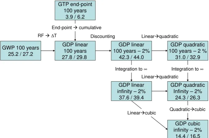
Fig. 1. Sensitivity of the methane CO2-equivalence (without/with the conversion of methane into CO2) to the construction of the climate
metric (see text for more details).
value of 25. This is consistent with the finding of Fuglestvedt et al. (2003), who showed how discount rate and damage function exponent can be combined to produce a methane GDP that is equivalent to the methane GWP for a given time horizon. This similarity in values for a quadratic dam-age function and a discount rate of 2 % and a time horizon of 100 yr can be explained through a number of compensat-ing effects (as illustrated in Fig. 1). Considercompensat-ing a cumula-tive function of the GMST change rather than a cumulacumula-tive function of RF increases the methane CO2-equivalence only
slightly. Discounting contributes to increase the methane CO2-equivalence substantially (i.e. by 14–15 units for a
lin-ear GDP and a time horizon of 100 yr) by giving more weight to the earlier climate impacts of methane. Integrating the methane and CO2 AGDP to infinity rather than to a 100-yr
time horizon only decreases the methane CO2-equivalence
by about 5 units because of the effect of discounting. Going from a linear to a quadratic damage cost function decreases the methane CO2-equivalence by about 13 units from 37.6
and 39.4 to 24.3 and 26.3. Overall, the compensation of ef-fects between the 100-yr GWP and our simple GDP is mostly between the opposing effects of discounting at a rate of 2 % and going from a linear to a quadratic damage cost function. The effect is much larger when going from an end-point GTP to a cumulative function of GMST change over 100 yr, as already noted by Gillett and Matthews (2010). Whether a pulse emission metric measures an end-point or a cumula-tive quantity is therefore a key factor differentiating existing metrics, at least for the longer time horizons
The large differences in GDP evaluated for linear, quadratic and cubic damage functions should be noted, with
values of 37.6/39.4, 24.3/26.3 and 14.4/16.5, respectively. These values are larger than those of Hammitt et al. (1996) and Kandlikar (1996), but the sensitivities to parameters are similar. As discussed above, there is little literature to jus-tify one or the other value for the exponent, but a quadratic function is often used.
3.2 Future evolution in methane CO2-equivalence
The methane GWP can vary in time, because the atmospheric residence times and radiative efficiencies of marginal pulses in CO2and CH4change over time. Previous authors have
in-vestigated how the GWP and GTP evolve for different but constant-in-time background levels, and similar changes can be expected for time-varying changes in the background lev-els. Caldeira and Kasting (1993) found that the decreasing radiative efficiency of CO2when the concentration increases
compensates for an increase in atmospheric residence time, as the ability of the ocean to absorb CO2 decreases. This
question was revisited by Reisinger et al. (2011), who found that the 100-yr absolute GWP of CO2 can be expected to
decrease as the CO2 background concentration increases.
Changes in methane residence time and radiative efficiencies can also affect its GWP (Br¨uhl, 1993). Reisinger et al. (2011) estimated that the 100-yr methane GWP can change by up to 20 % due to the combined effects of future changes in radia-tive efficiencies and residence times of CO2and CH4. The
O. Boucher: The methane CO2equivalence 55
background (fixed) concentrations and climate in the GWP calculations, they did not attempt to include time-evolving concentrations and climate in the GWP calculation itself. However, we can expect these effects to be of similar mag-nitude, and we estimate a±20 % range in the methane GWP due to changes in the CH4and CO2radiative efficiencies and
atmospheric lifetimes in future climates.
As anticipated earlier, the GDP increases with the start-ing time for the GDP calculation (variablet in Eq. 3, which is different from a time horizon). For our choice of central value parameters (i.e. a quadratic damage cost function and a 2 % discount rate), the GDP increases from a present-day value of 24.3 to 34.6 in 100 yr and 37.6 in 200 yr. This in-crease is due to the convexity of the damage cost function in a warming climate.
Other climate metrics can also be time-evolving. For in-stance, the methane CO2-equivalence implied by the GTP
increases when the time horizon is shortened as the climate target is approached. Global cost potential (e.g. Manne and Richels, 2001) or variants of the GTP (e.g. Johansson, 2012) are also designed to evolve with time. Generally speaking, there is some rationale for the methane CO2-equivalence to
increase with time, as climate change becomes more of a problem or is going to require more and more effort to com-bat. It is nevertheless possible to construct a climate metric where the methane CO2-equivalence decreases with time or
goes up and down, as discussed further in Sect. 3.5. This is the case, for instance, if a constraint on the rate of climate change is added to the climate metric (Manne and Richels, 2001). It is also possible that increased knowledge calls for some revision on the climate policy, which as a result brings down the methane CO2-equivalence. This would be the case,
for instance, if the climate sensitivity turns out to be less than expected (which would buy society some time) or if a thresh-old has been passed unintentionally and there is limited ad-ditional damage to be expected until one approaches the next threshold.
3.3 Sensitivity to individual parameters
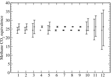
Figure 2 shows the ranges in methane GDP when each of the input parameters are varied within some reasonable range and all other parameters are held to their central values (see Table 1). For parameters that follow a Gaussian distribution, we vary the parameters within±2σfor this sensitivity study. The GDP, as we defined it, shows very little sensitivity to the details of the climate impulse response function and the methane to CO2conversion factor. It has a medium
sensitiv-ity to uncertainties in the O3and H2O enhancement factors
and the CO2radiative forcing, a somewhat larger sensitivity
to the the uncertainties on the methane perturbation lifetime and the underlying warming scenario. Finally, it exhibits a large sensitivity to the shape of the temperature damage func-tion (our exponentγ) and the largest sensitivity to the choice of discount rateρwithin the 1 to 3 % range. It is notable that
1 2 3 4 5 6 7 8 9 10 11 12
0 5 10 15 20 25 30 35 40
Methane CO
2
equivalence
Fig. 2. Uncertainty range in the methane GDP without and with methane conversion when individual parameters from Table 1 (listed from 1 to 12) are varied within the ranges specified in the Table and all other parameters are held to their central values. The central values are 24.3 and 26.3 without and with CH4conversion to CO2, respectively.
Fig. 2. Uncertainty range in the methane GDP without and with
methane conversion when individual parameters from Table 1 (listed from 1 to 12) are varied within the ranges specified in the table and all other parameters are held to their central values. The
central values are 24.3 and 26.3 without and with CH4conversion
to CO2, respectively.
the largest sensitivity is from the choice of socio-economic parameters, which are potentially less constrained and more value-laden than the physical parameters.
3.4 Total uncertainty
Although the choices of the central value and range are guided by the existing literature, we recognize that there is some degree of expert and value judgement in some of these parameters. We run a 10 000 point Monte Carlo calculation that sample the uncertainties in all of these variables (as-suming errors are independent), which affect the methane GWP, GTP and GDP. Because we consider a large number of parameters, the overall uncertainty is not overly sensitive to small variations in the uncertainty ranges that could arise from a particular expert judgement.
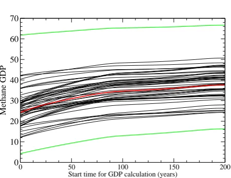
Figure 3 shows how the 50 first members of the Monte Carlo simulation evolve over time, along with our minimum, maximum and central values for the GDP. The kink that oc-curs around year 100 in some of the members is because of the change in the rate of global warming in that year, as evi-dent from Eq. (4). One can note that the increase in GDP over the next 200 yr is largest for the smallest present-day GDP, at least in relative terms. A smaller present-day methane CO2
-equivalence implies a steeper relative increase over time in the next 100 yr. The rest of the section is now focused on the present-day GDP value.
Table 2. Minimum, maximum, central values, mean, standard deviation, 1–99 % and 5–95 % uncertainty ranges for the 100-yr GWP, 100-yr
GTP and GDP.
Metric Minimum Maximum Central Value Mean Standard 1–99 % 5–95 %
(Median) Deviation Range Range
100-yr GWP w/o CO2 16.4 37.3 25.2 25.3 2.8 19.0–32.5 20.5–30.5
100-yr GWP w CO2 17.9 39.8 27.2 27.3 2.8 21.0–34.5 22.5–32.5
100-yr GTP w/o CO2 1.0 12.3 3.9 4.1 1.8 1.5–7.5 2.0–6.5
100-yr GTP w CO2 2.6 15.1 6.2 6.3 1.8 4.0–10.0 4.5–9.0
GDP w/o CO2 4.3 61.8 24.3 24.7 6.7 10.0–42.5 12.5–38.0
GDP w CO2 5.9 63.9 26.3 26.7 6.7 12.5–44.5 15.0–40.0
O. Boucher: The methane CO2equivalence 17
0 50 100 150 200
Start time for GDP calculation (years) 0
10 20 30 40 50 60 70
Methane GDP
Fig. 3. Methane GDP as a function of the start time for the first 50 members of our Monte-Carlo simulations when randomly perturbing the input parameters with the PDFs specified in Table 1. The red line is for our best guess estimate and the green lines are for the minimum and maximum values for input parameters as specified in Table 1. The figure shows the case without the CH4conversion to CO2.
Fig. 3. Methane GDP as a function of the start time for the first 50
members of our Monte Carlo simulations when randomly perturb-ing the input parameters with the PDFs specified in Table 1. The red line is for our best guess estimate and the green lines are for the minimum and maximum values for input parameters, as specified
in Table 1. The figure shows the case without the CH4conversion
to CO2.
confidence interval in the methane 100-yr GTP (2.0–6.5) is significantly different to the (3.9–13.5) range reported by Reisinger et al. (2010). This appears to be due to differences in the methane AGTP rather than in the CO2AGTP. The
dis-crepancy may partly be explained by the fact that Reisinger et al. (2010) include the effect of the climate-carbon feed-back in their calculation of the methane AGTP, when we do not. Further work is required to understand the differences in methane GTP from different authors.
The median values for the GDP are the same as the central values quoted above. The uncertainty on the methane GDP is significant with a standard deviation of 6.7. It is significantly larger than the uncertainty on the 100-yr GWP and GTP, for which the standard deviations are 2.8 and 1.8, respectively. In that sense, it is a less robust climate metric than GWP, but it offers more flexibility for adjustment (on e.g. the shape of
18 O. Boucher: The methane CO2equivalence
0 10 20 30 40 50 60
CH4 GWP / GTP / GDP 0
0.05 0.1 0.15 0.2
Probability
GWP100 GTP
100
GDP
GWP100 with CO2 effect GTP100 with CO2 effect GDP with CO
2 effect
Fig. 4. Probability distribution function of the methane CO2-equivalence (GWP with 100 years time horizon, GTP with 100 years time horizon, and GDP) obtained from randomly perturbing the input parameters with the PDFs specified in Table 1. The dashed lines account for the CHFig. 4. Probability distribution function of the methane CO4conversion to CO2. 2
-equivalence (GWP with 100-yr time horizon, GTP with 100-yr time horizon, and GDP) obtained from randomly perturbing the input pa-rameters with the PDFs specified in Table 1. The dashed lines
ac-count for the CH4conversion to CO2.
damage function and the discount rate) as our knowledge on climate change and its impacts progress, as already noted by Hammitt et al. (1996).
The maximum values for the methane GDP, which can be obtained from the parameter ranges in Table 1, are 61.8 and 63.9 without and with the CH4conversion to CO2,
re-spectively. This maximum value is about 2.5 times larger than the 100-yr GWP for methane. The minimum values for the methane CO2-equivalence that can be built are 4.3
and 5.9 without and with CH4 conversion to CO2,
respec-tively. This is 5 to 6 times less than the 100-yr GWP, but fairly close to the central value for the 100-yr GTP. These minimum and maximum values for the methane GDP are ac-tually well outside the 1–99 % uncertainty ranges, which are 10.0–42.5 and 12.5–44.5 without and with the CO2
O. Boucher: The methane CO2equivalence 57
3.5 Sensitivity to some structural uncertainties
We investigate here the sensitivity of our results to some of the structural uncertainties embedded in the GDP met-ric. As noted earlier, there is no consensus on the shape of the damage function and an exponent function was chosen for simplicity. Other shapes have been proposed, such as a hockey stick (Tol et al., 1998), an S-shaped or sigmoid func-tion (Ambrosi et al., 2003) or a sum of sigmoid funcfunc-tions. Hockey-stick damage functions may be appropriate in cost-benefit analysis (they essentially imply that there is a thresh-old GMST change, above which we should mitigate at any cost), but would cause some inconsistency in the GDP calcu-lation as the temperature change trajectory is prescribed in-dependently from the damage function. Therefore, we only consider sigmoid damage functions here as an alternative to an exponent function. The sigmoid damage function in arbi-trary unit can be written as
D(1T )=1+tanh
1T −1T
1
dT
(9) where1T1 is a threshold temperature change and dT
de-fines the stiffness of the changes around the threshold (taken to be 0.5◦C). With such a damage function, the impacts are initially small and then increase sharply before reaching a plateau. Although the plateau may not be a realistic feature, a sigmoid function represents the existence of a threshold around a given GMST change. We use a value1T1of 2◦C
and the lower bound of our warming scenario as a sensitivity test. We also consider the sum of two or three sigmoid func-tions centred on thresholds of 4 and 6◦C and associated with double and triple damages:
D(1T )=1+tanh
1T −1T
1 dT
+2 tanh
1T−1T
2 dT
(10) and
D(1T )=1+tanh
1T −1T
1 dT
+2 tanh
1T −1T
2 dT
+3 tanh
1T−1T
3 dT
. (11)
These damage functions are considered along with our me-dian and upper bound warming scenarios, respectively. It should be noted that a damage function that corresponds to multiple thresholds of increasing severity becomes similar in shape to an exponent function.
Figure 5 shows the time evolution of the methane CO2
-equivalence for a range of climate metrics, including those corresponding to the sigmoid damage functions defined above. For the GWP and GTP metrics, we show how the CO2-equivalence would increase if the time horizon is
short-ened from 100 yr down to 1 yr. This implies a faster increase in time than for any of the exponent functions chosen here. It also appears that the use of a sigmoid or a sum of sigmoids
0 50 100 150 200
Time in the future (years) 0
10 20 30 40 50 60 70 80 90 100
Methane CO
2
-equivalence
γ=1 ρ=2% median γ=2 ρ=2% median γ=3 ρ=2% median 1 sigmoid minimum 2 sigmoids median 3 sigmoids maximum GWP decreasing time horizon GTP decreasing time horizon
Fig. 5. Time evolution of the methane CO2-equivalence for a set of climate metrics: GDP with linear, quadratic and cubic damage functions, GDP with one sigmoid damage function, GDP with the sum of two or three sigmoid damage functions, GWP with decreasing time horizon (from 100 years to 1 year), GTP with decreasing time horizon (from 100 years to 1 year). The legend box indicates if the minimum, median or maximum warming scenario was used. The figure shows the case without the CH4conversion to CO2.
Fig. 5. Time evolution of the methane CO2-equivalence for a set of
climate metrics: GDP with linear, quadratic and cubic damage func-tions, GDP with one sigmoid damage function, GDP with the sum of two or three sigmoid damage functions, GWP with decreasing time horizon (from 100 yr to 1 yr), GTP with decreasing time hori-zon (from 100 yr to 1 yr). The legend box indicates if the minimum, median or maximum warming scenario was used. The figure shows
the case without the CH4conversion to CO2.
for the damage function can result in up and down for the methane CO2-equivalence, but these stay in the same range
as for the exponent damage functions. A smaller value for dT would result in a larger range of values; however, there is little literature to support the concept of a rapid transition around a threshold under future global warming.
It has been argued that damage from climate change is also a function of the rate of change (Tol, 1996; O’Neill and Oppenheimer, 2004). Manne and Richels (2001) have shown how this translates into the methane CO2-equivalence
for their metric. However, there is little quantitative informa-tion on how damage responds to the rate of climate change. Moreover, incorporating a constraint on the rate of change can only be done properly if the concentration pathways of both long-lived and short-lived climate forcers are optimized, which is not compatible with the simple approach taken here with the GDP. For these reasons we do not attempt to further examine this issue.
rate of 2 % with GDP values of 20.0 and 22.0 without and with the CH4to CO2conversion effect, respectively. We also
test extreme values of the discount rates of 0.5 % and 5 %, with corresponding GDP values 7.8/9.9 and 49.6/51.2, re-spectively. However, it should be noted that such values find little support in the scientific literature on the economics of climate change.
4 Interpreting the methane CO2-equivalence
Most climate metrics that have been defined are for pulse emissions. Climate metrics for sustained emissions have been proposed (e.g. Shine et al., 2005) and used in some studies (e.g. Jacobson, 2002; Dessus et al., 2008). Metrics for sustained emissions give larger CO2-equivalences than
their pulse emission counterpart for short-lived species such as methane or black carbon (Shine et al., 2005). It is some-times argued that a metric for sustained emissions should be used to trade perennial emission reductions. To disprove this we introduce a generalised sustained GDP (denoted GDPs),
which compares the relative discounted climate effects of CH4and CO2emissions overnyears:
GDPs= n−1
P
t=0
AGDPCH4(t )/(1+ρ)
t
n−1 P
t=0
AGDPCO2(t )/(1+ρ)t
=
n−1 P
t=0
∞ R
t0=0
D 1T (t+t0)+δT
CH4(t
0)
−D(1T (t+t0))
/(1+ρ)t+t0
dt0
n−1 P
t=0
∞ R
t0=0
D 1T (t+t0)+δTCO2(t
0)
−D(1T (t+t0))
/(1+ρ)t+t0
dt0
. (12)
It should be noted that the individual pulses do not add to the
1T trajectory in this equation.
Let us try to reconcile the viewpoint of a policymaker who wants to define an equivalence between CH4 and CO2 that
is based on a climate target and the viewpoint of an investor who wants to maximize the value of their investment in the context of the financial tools set up by the policymaker. We assume there is an upfront cost,XCH4, and a running cost, YCH4(t ), to reduce CH4emissions by 1 kg yr
−1, and likewise
for 1 kg yr−1of CO2, with the costs being notedXCO2 and YCO2(t ).
The investor wants to pay back their investment by avoid-ing payavoid-ing a greenhouse gas tax or buyavoid-ing emission credits, or by selling emission credits if emissions were reduced be-yond expectation. In a fluid market, emission reductions will take place at increasing costs until
XCO2+
n−1 X
t=0
YCO2(t )/(1+ρ)
t = n−1 X
t=0
PCO2(t )/(1+ρ)
t (13)
wherePCO2(t )is the price of 1 kg of CO2, which evolves
over time. We have discounted both the CO2price and the
CO2 emission reduction cost to reflect uncertainties on the
future. The discount rate needs not to be the same as in Eq. (3) as long as it is the same discount rate used in the LHS and RHS of Eq. (13). One can then write an analogous equation to Eq. (13) but for CH4emission reductions.
Ratio-ing the two equations gives
XCH4 + n−1
P
t=0
YCH4(t )/(1+ ρ) t
XCO2 + n−1
P
t=0
YCO2(t )/(1+ρ) t
=
n−1
P
t=0
PCH4(t )/(1+ρ) t
n−1
P
t=0
PCO2(t )/(1+ρ) t
(14)
wherePCH4(t )is the price of 1 kg of CH4, which can also
evolve over time.
For the policy to be most effective, the policymaker wants the ratio of the discounted CH4and CO2prices to be equal
to the ratio of their climate benefits:
n−1
P
t=0 ∞
R
t0=0
D 1T (t+t0)+δTCH4(t
0 )
−D(1T (t+t0))
/(1+ρ)t+t0dt0
n−1
P
t=0 ∞
R
t0=0
D 1T (t+t0
)+δTCO2(t
0 )
−D(1T (t+t0 ))
/(1+ρ)t+t0 dt0
=
n−1 P
t=0
PCH4(t )/(1+ρ)
t
n−1 P
t=0
PCO2(t )/(1+ρ)t
. (15)
Noting,RCH4(t ), the ratio between the CH4and CO2prices,
the previous equation becomes n−1
P
t=0
AGDPCO2(t )GDPCH4(t )/(1+ρ)
t
n−1 P
t=0
AGDPCO2(t )/(1+ρ)t
=
n−1 P
t=0
PCO2(t ) RCH4(t )/(1+ρ)
t
n−1 P
t=0
PCO2(t )/(1+ρ)t
. (16)
The equation above is verified if the variations of PCO2(t )
follow those of AGDPCO2(t )and if the variations ofRCH4(t )
follow those of GDPCH4(t ). Said differently, the price of CO2
needs to increase as the absolute GDP of CO2increases over
time, and the CO2-equivalence of methane for pulse emission
needs to increase as its GDP increases over time. The investor can then use Eqs. (13) and (14) to optimise their strategy for emission reductions.
There are several implications of the above: (i) there is no scientific reason for the methane CO2-equivalence to be
con-stant over time; (ii) there is no need to introduce a metric for sustained emissions as long as the methane CO2-equivalence
for pulse emission evolves over time; and (iii) there needs to be enough visibility from policymakers on how the price of CO2and the methane CO2-equivalence are going to vary
CO2and CH4investment in a way that is effective for
min-imising the impacts of climate change. It should be noted that the conclusions reached here hold even if a different pulse climate metric had been used to calculate the methane CO2
-equivalence.
5 Conclusions
We defined a simplified GDP for methane as the ratio of the discounted cumulative climate change impacts due to the pulse emission of 1 kg of methane relative to 1 kg of CO2.
The simplified GDP is a function of 12 parameters, which we have varied in order to explore the sensitivity of the methane CO2-equivalence to various parameter choices. We produced
a probability distribution function for the methane GDP by varying input parameters within some reasonable ranges.
Our findings can be summarised as follows:
1. If the damage cost function is a convex function of the GMST change, as it is usually considered, the methane GDP increases as global warming unfolds. The GDP (as defined here) can be used consistently as we approach and go past a climate target in a stabilisation scenario. 2. The median value of the methane GDP is 24.3, which is
very close to the 100-yr methane GWP. This is because replacing the cumulative function of the RF in the GWP with a quadratic function of the GMST in the GDP is compensated by the introduction of a 2 % discount rate, which gives more importance to the short lifetime of methane.
3. There is a large spread in our GDP calculations (larger than the spread in GWP and GTP) when we vary in-put parameters within some reasonable ranges. The largest uncertainties come from uncertainties or judge-ment value on two economic parameters: the degree of convexity of the damage cost function and the discount rate. It should be noted that the choice of the discount rate is related to the choice of a time horizon when the GWP or GTP metric is used.
4. The 1–99 % uncertainty ranges for the methane GDP are 10.0–42.5 and 12.5–44.5 without and with the CH4
to CO2conversion effect, respectively. This uncertainty
range only includes parametric uncertainties and not structural uncertainties. It should be noted however that the analysis spans rather large intervals of parametric uncertainties.
5. The main factor differentiating the methane 100-yr GTP from the methane 100-yr GWP and the GDP is the fact that the former metric is an end-point metric, whereas the latter are cumulative metrics. More work is required to understand differences in the methane GTP estimates between different authors.
6. There is some rationale for an increase in the methane CO2-equivalence in the future as global warming
un-folds. This is implied by a convex damage function, in the case of the GDP metric or by shortening the time horizon as the climate target is approached in the case of an end-point metric such as the GTP. The ensemble GDP calculation suggests that the relative increase is more for the smaller values of the GDP.
7. Reconciling the legitimate objectives of a policymaker and an investor willing to invest money in order to de-crease CH4emissions in the long term requires that both
the price of CO2and the methane CO2-equivalence for
a pulse emission vary over time in some known and visible way. There is no need for policy-makers to in-troduce an additional metric for sustained emission to make perennial investment decisions as long as there is enough visibility on future prices and CO2-equivalences
for the stakeholders.
Our GDP remains a simplified metric. One assumption in particular merits more investigation. Climate impacts vary geographically and across activities, and parametrising the damage cost function as a power of the GMST is probably an oversimplification. Moreover, there is an increasing recogni-tion that different species have different impacts on the Earth system. For instance, CO2 has a radiative effect, a
fertilisa-tion effect on plants and an acidificafertilisa-tion effect on the ocean, while CH4has an indirect effect on ozone, which may further
affect the carbon cycle (Collins et al., 2010). These different effects may result in different impacts on ecosystem services, and this needs to be factored in climate metrics (Hunting-ford et al., 2011). Finally, the very large sensitivity to the dis-count rate suggests that more work should be done to better frame this concept into socio-economic scenarios for climate change adaptation and mitigation.
Acknowledgements. O. B. would like to thank two anonymous
referees, Andy Reisinger, Glen Peters and Jan Fuglestvedt for their useful comments on the discussion paper.
Edited by: P. Friedlingstein
References
Ambrosi, P., Hourcade, J.-C., Hallegatte, S., Lecocq, F., Dumas, P., and Ha-Duong, M.: Optimal control models and elicitation of at-titudes towards climate change, Environ. Model. Assess., 8, 135– 147, 2003.
Boucher, O.: Quel rˆole pour les r´eductions d’´emission de m´ethane dans la lutte contre le changement climatique?, La M´et´eorologie, 68, 35–40, 2010.
Boucher, O., Friedlingstein, P., Collins, B., and Shine, K. P.: Indirect GWP and GTP due to methane oxidation, Environ. Res. Lett., 4, 044007, doi:10.1088/1748-9326/4/4/044007, 2009.
Br¨uhl, C.: The impact of the future scenarios for methane and other chemically active gases on the GWP of methane, Chemosphere, 26, 731–738, 1993.
Caldeira, K. and Kasting, J. F.: Insensitivity of global warming po-tentials to carbon dioxide emission scenarios, Nature, 366, 251– 253, 1993.
Collins, W. J., Sitch, S., and Boucher, O.: How vegetation impacts affect climate metrics for ozone precursors, J. Geophys. Res., 115, D23308, doi:10.1029/2010JD014187, 2010.
Dessus, B., Laponche, B., and Le Treut, H.: R´echauffement clima-tique: importance du m´ethane, La Recherche, 417, 46–49, 2008. Forster, P., Ramaswamy, V., Artaxo, P., Berntsen, T., Betts, R. A., Fahey, D. W., Haywood, J. A., Lean, J., Lowe, D. C., Myhre, G., Nganga, J., Prinn, R., Raga, G., Schulz, M., and Van Dorland, R.: Changes in atmospheric constituents and in radiative forcing, in: Climate Change 2007: The Physical Science Basis, Contribu-tion of Working Group I to the Fourth Assessment Report of the Intergovernmental Panel on Climate Change, Cambridge Univer-sity Press, 129–234 pp., 2007.
Fuglestvedt, J. S., Berntsen, T. K., Godal, O., Sausen, R., Shine, K. P., and Skodvin, T.: Metrics of climate change: assessing radia-tive forcing and emission indices, Climatic Change, 58, 267–331, 2003.
Fuglestvedt, J. S., Shine, K. P., Berntsen, T., Cook, J., Lee, D. S., Stenke, A., Skeie, R. B., Velders, G. J. M., and Waitz, I. A.: Transport impacts on atmosphere and climate: metrics, Atmos. Environ., 44, 4648–4677, 2010.
Gillenwater, M.: Forgotten carbon: indirect CO2in greenhouse gas
emission inventories, Environ. Sci. Policy, 11, 195–203, 2008. Gillett, N. P. and Matthews, H. D.: Accounting for carbon
cy-cle feedbacks in a comparison of the global warming ef-fects of greenhouse gases, Environ. Res. Lett., 5, 030411, doi:10.1088/1748-9326/5/3/034011, 2010.
Hallegatte, S.: A Proposal for a New Prescriptive Discount-ing Scheme: The Intergenerational Discount Rate, Fondazione Eni Enrico Mattei Working Papers, Working Paper 206, avail-able from http://www.bepress.com/feem/paper206, (last access: 27 March 2012), 2008.
Hammitt, J. K., Jain, A. K., Adams, J. L., and Wuebbles, D. J.: A welfare-based index for assessing environmental effects of greenhouse-gas emissions, Nature, 381, 301–303, 1996. Hansen, J., Sato, M., Ruedy, R., Lacis, A., and Oinas, V.: Global
warming in the twenty-first century: An alternative scenario, Proc. Natl. Acad. Sci. USA, 97, 9875–9880, 2000.
Heal, G.: Discounting and climate change: an editorial comment, Climatic Change, 37, 335–343, 1997.
Huntingford, C., Cox, P., Mercado, L., Sitch, S., Bellouin, N., Boucher, O., and Gedney, N.: Highly contrasting effects of differ-ent climate forcing agdiffer-ents on ecosystem services, Philos. T. Roy. Soc. A, 369, 2026–2037, doi:10.1098/rsta.2010.0314, 2011. IPCC: 2006 IPCC Guidelines for National Greenhouse Gas
Inven-tories, available from http://www.ipcc-nggip.iges.or.jp/public/ 2006gl/index.html (ast access: 17 May 2012), 2006.
IPCC: Contribution of Working Group I to the Fourth Assess-ment Report of the IntergovernAssess-mental Panel on Climate Change, 2007, edited by: Solomon, S., Qin, D., Manning, M., Chen, Z.,
Marquis, M., Averyt, K. B., Tignor, M., and Miller, H. L., Cam-bridge University Press, CamCam-bridge, UK and New York, NY, USA, 2007.
IPCC: Meeting Report of the Expert Meeting on the Science of Al-ternative Metrics, edited by: Plattner, G.-K., Stocker, T. F., Midg-ley, P., and Tignor, M., IPCC Working Group I Technical Support Unit, University of Bern, Bern, Switzerland, 75 pp., 2009. Jacobson, M. Z.: Control of fossil-fuel particulate black
car-bon and organic matter, possibly the most effective method of slowing global warming, J. Geophys. Res., 107, 4410, doi:10.1029/2001JD001376, 2002.
Johansson, D. J. A.: Economics- and physical-based metrics for comparing greenhouse gases, Climatic Change, 110, 123–141, 2012.
Kandlikar, M.: Indices for comparing greenhouse gas emissions: integrating science and economics, Energy Econ., 18, 265–282, 1996.
Manne, A. S. and Richels, R. G.: An alternative approach to es-tablishing trade-offs among greenhouse gases, Nature, 410, 675– 677, 2001.
Nordhaus, W. D.: Discounting in economics and climate change: an editorial comment, Climatic Change, 37, 315–328, 1997. O’Neill, B. C. and Oppenheimer, M., Climate change impacts are
sensitive to the concentration stabilization path, P. Natl. Acad. Sci. USA, 101, 16411–16416, 2004.
Pearce, D., Groom, B., Hepburn, C., and Koundouri, P.: Valuing the future, recent advances in social discounting, World Econom., 4, 121–141, 2003.
Peters, G. P., Aamaas, B., Bernsten, T., and Fuglestvedt, J.: The inte-grated global temperature change potential (iGTP) and relation-ships between emission metrics, Environ. Res. Lett., 6, 044021, doi:10.1088/1748-9326/6/4/044021, 2011.
Ramaswamy, V., Boucher, O., Haigh, J., Hauglustaine, D., Hay-wood, J., Myhre, G., Nakajima, T., Shi, G., and Solomon, S.: Radiative Forcing of Climate Change, IPCC Third Assessment Report Climate Change 2001: The Scientific Basis, edited by: Houghton, J. T., Ding, Y., Griggs, D. J., Noguer, M., van der Lin-den, P. J., Dai, X., Maskell, K., and Johnson, C. A., Cambridge University Press, Cambridge, UK and New York, USA, 349–416, 2001.
Reisinger, A., Meinshausen, M., Manning, M., and Bodeker, G.:
Uncertainties of global warming metrics: CO2 and CH4,
Geo-phys. Res. Lett., 37, L14707, doi:10.1029/2010GL043803, 2010. Reisinger, A., Meinshausen, M., and Manning, M.: Future changes in global warming potentials under representative concentra-tion pathways, Environ. Res. Lett., 6, 024020, doi:10.1088/1748-9326/6/2/024020, 2011.
Sherwood, S. C., Discounting and uncertainty – A non-economist’s view, Climatic Change, 80, 205–212, 2007.
Shine, K. P.: The global warming potential – the need for an inter-disciplinary retrial, Climatic Change, 96, 467–472, 2009. Shine, K. P., Fuglestvedt, J. S., Hailemariam, K., and Stuber, N.:
Al-ternatives to the global warming potential for comparing climate impacts of emissions of greenhouse gases, Climatic Change, 68, 281–302, 2005.
Stern, N.: Stern Review on The Economics of Climate Change, HM Treasury, London, available from http://www.hm-treasury.gov. uk/sternreview index.htm, (last access: 12 January 2012), 2007. Tol, R. S. J., The damage costs of climate change towards a dynamic
representation, Ecol. Econom., 19, 67–90, 1996.
Tol, R. S. J. and Fankhauser, S.: On the representation of impact in integrated assessment models of climate change, Environ. Model. Assess., 3, 63–74, 1998.
Tol, R. S. J., Berntsen, T. K., O’Neill, B. C., Fuglestvedt, J. S., Shine, K. P., Balkanski, Y., and Makra, L.: A unifying frame-work for metrics for aggregating the climate effect of differ-ent emissions, ESRI Working Paper 257, Economic and Social Research Institute, Dublin, Irland, http://www.esri.ie/UserFiles/ publications/20080924144712/WP257.pdf, (last access: 12 Jan-uary 2012), 2008.
UK Green Book, Appraisal and Evaluation in Central Government, Treasury Guidance, available from http://www.hm-treasury.gov. uk/d/green book complete.pdf, (last access: 27 March 2012), 2011.
van Vuuren, D. P., Weyant, J., and de la Chesnaye, F.: Multi-gas sce-narios to stabilize radiative forcing, Energy Econom., 28, 102– 120. 2006.
Warren, R., Hope, C., Mastrandrea, M., Tol, R., Adger, N., and Lorenzoni, I.: Spotlighting Impacts Functions in Inte-grated Assessment, Research Report Prepared for the Stern Review on the Economics of Climate Change, available from http://www.tyndall.ac.uk/content/spotlighting, last access: 12 January 2012, Tyndall Centre for Climate Change Research, Working Paper 91, September 2006.
Weitzman, M. L.: A review of the Stern Review on the economics of climate change, J. Econom. Literat., XLV, 703–724, 2007. Weitzman, M. L.: What is the “damages function” for global