Published online July 10, 2013 (http:// www.sciencepublishinggroup.com/j/ijepp) doi: 10.11648/j.ijepp.20130102.11
CFD based parametric analysis of gas flow in a
counter-flow wet scrubber system
Bashir Ahmed Danzomo
1, *, Momoh-Jimoh Enyiomika Salami
1, Raisuddin Mohd Khan
1,
Mohd Iskhandar Bin Mohd Nor
21Department of Mechatronics Engineering, International Islamic University, P. O. Box 10, 50728, Kuala Lumpur, Malaysia
2Chemical Engineering Department, University of Malaya, 50603, Kuala Lumpur, Malaysia
Email address:
[email protected](B. A. Danzomo)
To cite this article:
Bashir Ahmed Danzomo, Momoh-Jimoh Enyiomika Salami, Raisuddin Mohd Khan, Mohd Iskhandar Bin Mohd Nor. CFD Based Para-metric Analysis of Gas Flow in A Counter-Flow Wet Scrubber System. International Journal of Environmental Protection and Policy.Vol. 1, No. 2, 2013, pp. 16-23. doi: 10.11648/j.ijepp.20130102.11
Abstract:
Environmental protection measures regarding industrial emissions and tightened regulations for air pollution led to the selection of a counter-flow wet scrubber system based on applicability and economic considerations.The flow dynamics of gas transporting particulate matter and gaseous contaminants is a key factor which should be considered in the scrubber design. In this study, gas flow field were simulated using ANSYS Fluent computational fluids dynamic (CFD) software based on the continuity, momentum and k-ε turbulence model so as to obtain optimum design of the system, im-prove efficiency, shorten experimental, period and avoid dead zone. The result shows that the residuals have done a very good job of converging at minimum number of iterations and error of 1E-6. The velocity flow contours and vectors at the inlet, across the scrubbing chamber and the outlet shows a distributed flow and the velocity profiles have fully conformed to the recommended profile for turbulent flows in pipes. The total pressure within the scrubber cross-section is constant while the minimum and maximum pressure drops was obtained to be 0.30pa and 3.03pa which has conformed to the rec-ommended pressure drop for wet scrubbers. From the results obtained, it can be deduced that the numerical simulation us-ing CFD is an effective method to study the flow characteristics of a counter-flow wet scrubber system.Keywords:
Computational Fluid Dynamics, Counter-Flow Wet Scrubber, Parametric Analysis, Gas Flow1. Introduction
A counter-flow wet scrubber system is an air pollution control device that uses liquid spray to control particles contained in a particulate matter (PM) and gaseous con-taminants that are being emitted from industrial production. The simplest type of the scrubber is the cylindrical or rec-tangular system in which air and contaminants passes into a chamber where it contacts a liquid spray produced by spray nozzles located across the flow passage. As indicated by [1], counter-flow scrubbers have important advantage when compared to other air pollution control devices. They can collect flammable and explosive dusts safely, absorb gase-ous pollutants, collect mists, cool hot gas streams and it has the potential to save 35 to 40 percent over the cost of con-ventional air pollution control equipment for brick kilns while meeting new standards for the control of waste gas (dust) emissions from cement fabrication, hydrogen fluoride, hydrogen chloride (HCl) and particulate matter (PM) [1].
produces better designs. Hudson [3], Kennedy et al. [4] and Minghua et al. [5] indicated that, computational fluid dynamics (CFD) approach has promising applications in both dry and wet counter-flow scrubber systems for indus-trial air pollution applications. It has the benefit of devel-oping a virtual prototype which can evaluate and compare design alternatives without material, construction and test-ing cost, the advantage of enabltest-ing and improvtest-ing engi-neering design with tight margins, simulating complex fluid flow phenomena at a reduced cost and demonstrating project feasibility prior to construction as in [6,7,8,9].
The main objective of this study is to perform a CFD based parametric numerical analysis of the gas flow dy-namics of a counter-flow wet scrubber system so as to ex-plore the velocity and pressure field profiles and optimize the gas-PM flow in the scrubber system so as to avoid dead zone within the systems cross section.
2. Materials and Method
2.1. The Case Study Specifications
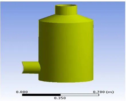
The studied wet scrubber has been designed using hy-draulic similitude method by considering data obtained from cement industry as shown in Table 1. Schematic diagram of the system is described in Figure 1.
Table 1. Summary of Kiln Shop Exhaust PM-Laden Gas Data
Operating Parameter Operating Data
Volume Flow Rate 104,885 m3/hr
Mass Flow 119,084 kg/hr
Gas Temperature 105 0C
Dust Burden (Inlet) 62,500 µg/m3
Dust Burden (Outlet) 25,000 µg/m3
Source: Ashaka Cement Company [10]
Figure 1. Geometric Sketch of the Scrubber
Considering the fact that, the scrubber gas outflow is our subject of concern in this study; a curved transition using hood design approach was provided so as to create shape and good flow characteristics of the gas out of the scrubber with minimum friction loss. However, this transition was not provided at the slurry exit, because its flow characteris-tics have not been considered in the study.
2.2. Mathematical Modeling
The appropriate governing equations for the gas flow are the incompressible Nervier Stokes Equation (NSE) for a single phase flow obtained from the conservation of mass and momentum described by Caiting, et al. [7].
Continuity equation
( )
=
0
∂
∂
i ix
U
(1) Momentum equation i g i j g j i g eff j i i j g i g g g x U x U x x P x U U ρ µ ρ + ∂ ∂ + ∂ ∂ ∂ ∂ + ∂ ∂ − = ∂ ∂( ) (2)Where, i and j are the direction vectors for the three co-ordinates (x, y, and z) while Ugi and Ugj are the three veloc-ity components (u, v, w) of the gas flow, µeff is the effec-tive dynamic viscosity of gas, ρgis the gas density, P is the gas pressure and ρgi is the gas volume force in i-direction respectively.
To avoid the unnecessary consumption of the computer time for the solution of the full-scale, turbulence model for predicting the effects of turbulence in the gas phase should be considered. Averaging is often used to simplify the solu-tion of the governing equasolu-tions of turbulence, but models are needed to represent scales of the flow that are not re-solved. One of the most effective viscosity models for the simulations of the turbulent flow is the Harlow-Nakayama
k-ε model of the turbulent flow described in (3) and (4). The model provides the time averaged values of velocities and pressure of the gas or air throughout the system.
k c x U x U x U k c x x x U equation i J j i j i t i i t i i 2 2 1 ) (
ε
ρ
µ
ε
ε
δ
µ
µ
ε
ρ
ε
ε − ∂ ∂ + ∂ ∂ ∂ ∂ + ∂ ∂ ∂ + ∂ = ∂ ∂ − (4)Where k is the turbulent kinetic energy, ε is the turbulent kinetic energy dissipation rate; µt is viscosity coefficient of turbulent flow while δk, δε, c1, c2 are constants; c1 = 1.44, c2 = 1.92, δk = 1.0, δε = 1.3 [7]. The standard k-ε model was based on the hypothesis of the isotropic eddy-viscosity, which was modeled through the flow fields of the turbulent kinetic energy and the specific dissipation rate. According to [11], the model leads to stable calculations that converg-es easily and allows reasonable predictions for many flows. Also, [7] indicated that k-ε is the most commonly used tur-bulence model which has many advantages; its concept is simple and it has been implemented in many commercial CFD codes. The model has demonstrated the capability to simulate many industrial processes effectively as in [6, 12, 13, and 14].
2.3. Numerical Computation Methods
A dimension of the scrubber in Figure 1 has been used to generate a 3D geometry of the scrubber system using CAD. The geometry was then imported into ANSYS Fluent [15] for processing.
As shown in Figure 2, the pipe geometry for the scrubbing liquid spray and the slurry outlet duct were suppressed from the main geometry so as to analyse only the gas flows across the scrubbing chamber.
Figure 2. Scrubber Geometries in ANSYS Fluent Workbench
Using the ANSYS Fluent [15] workbench and mesh windows the volume for the flow dynamics was filled and the boundary condition defined. The calculation domain of the scrubber geometry was applied to produce good mesh
profile by using efficient meshing parameters such as; the growth rate and mesh refinement as shown in Figure 3.
A growth rate of 1.4 and a refinement of 3 were used across the scrubber inlets, outlets and the wall parts so as to provide a smooth flow transition across the system.
Figure 3. Boundary Condition and Mesh Profile of the Scrubber Geome-tries
This yielded a statistics of 91,051 nodes and 459,870 elements and an aspect ratio of 5.98832 and skewness of 0.6078. However, these values are within the required range of mesh skewness ≤ 1.0 and aspect ratio ≤ 10 respec-tively. For the boundary condition, velocity inlet has been selected at the gas inlet while pressure outlet was chosen for the gas outlet.
Values for the inlet velocities were chosen from the range of USEPA and NACAA [16], Ngala et al. [17] and Garba [18] recommended PM transport velocities; 0.32, 0.79 and 1.27m/s. The simulation starts by identifying and applying conditions at the domain boundaries and then solving the governing equations on the computational mesh iteratively as a steady-state. Since this is a pressure based solution method, the PISO (Pressure Implicit with Splitting of Operators) algorithm recommended by ANSYS Fluent [19] for solving steady flow calculations (especially when the solution involves turbulence model) has been used. Also, [19] indicated that generally for triangular and tetrahedral meshes, a more accurate result is obtained by using the second-order discretization.
There are six differential equations to be solved in 3D which resulted to six residuals for convergence; continuity,
x-velocity, y-velocity, z-velocity and k-ε turbulent equations
1. The gas phase flow was only considered in the scrub-ber and no liquid phase is taken into account,
2. The flow is stable and isothermal, so heat exchange among the phase is not considered,
3. The gas is regarded as incompressible,
4. The PM transport velocity recommended by USEPA and NACAA [16] was considered for the simulation.
3. Results and Discussion
From the simulation experimentations, the residuals does a very good job of converging at approximately 590, 500, and 550 iterations at inlet velocities of 0.32, 0.79 and 1.27m/s as shown in Figures 4, 5 and 6.
Figure 4. Residuals for the Continuity, k-Epsilon and X, Y, Z Velocities at 0.32m/s
Figure 5. Residuals for the Continuity, k-Epsilon and X, Y, Z Velocities at 0.79m/s
Figure 6. Residuals for the Continuity, k-Epsilon and X. Y, Z at 1.27m/s
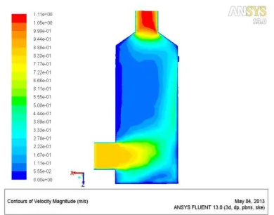
Graphic displays of the velocity fields which includes velocity contours describing the gas flows from the inlet, across the scrubbing camber to the outlet for the three inlet velocities considered in the study is shown in Figures 7, 8 and 9 (a and b)respectively.
Figure 7a. Y-Coordinate Contour Display of the Gas Flow across the Scrubber at 0.32m/s
Figure 7b. X-Coordinate Contour Display of the Gas Flow across the Scrubber at 0.32m/s
Figure 8b. X-Coordinate Contour Display of the Gas Flow across the Scrubber at 0.79m/s
Figure 9a. Y-Coordinate Contour Display of the Gas Flow across the Scrubber at 1.27m/s
Figure 9b. X-Coordinate Contour Display of the Gas Flow across the Scrubber at 0.79m/s
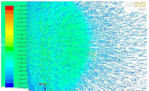
The velocity contours in X and Y coordinates above de-scribing the gas flow across the scrubber shows a more distributed flow across the spray chamber for a 0.32m/s velocity which are further supported by the velocity vector displays across the chamber shown in Figures 10, 11 and 12.
Figure 10. Velocity Vector of the Gas Flow within the Geometry
For the other velocities; 0.79 and 1.27m/s, the gas is par-tially distributed across the centre and fully distributed across the side walls.
Figures 10 and 11 shows a stream line flow along the scrubber inlet and the outlet ducts at 0.32m/s which have conformed to the Bernoulli’s theorem
Figure 11. Velocity Vector of the Gas Flow at Inlet 0.32m/s
Figure 12. Velocity Vector of the Gas Flow towards the Exit at 0.32m/s
Figure 13. Velocity Profile across a Cylindrical Pipe for Laminar and Turbulent Flows
As shown in figure 13, if the flow in a pipe is laminar, the velocity distribution at a cross section will be parabolic in shape with the maximum velocity at the centre being about twice the average velocity in the pipe.
In turbulent flow, a fairly flat velocity distribution exists across the section of pipe, with the result that the entire fluid flows at a given single value.
The velocity of the fluid in contact with the pipe wall is essentially zero and increases the further away from the wall. To validate the gas flow into the scrubber system, velocity profiles for the three velocities along the inlet duct was plotted as shown in Figures 14, 15 and 16.
Figure 14. Velocity Profile for the Inlet Gas at 0.32m/s
Figure 15. Velocity Profile for the Inlet Gas at 0.79m/s
Since turbulent model was considered in the CFD simu-lation, from the above figures it can be seen that the veloc-ity profiles has fully conformed to the recommended profile for turbulent flows in pipes and cylinders.
According to USEPA and NACAA [16], pressure drop
across a wet scrubber system is an important parameter in evaluating the performance and operations of the system especially for PM removal. The pressure drop is a meas-urement of the resistance to flow as the gas passes from one point to another point and is simply the arithmetic difference between the static pressure at the scrubber inlet and outlet (measured at right angles to the flow). The value of the pressure drop takes into account the amount of energy loos during wet scrubbing process. According to [22], the system pressure is computed using the gauge pressure (pressure measured in a system) and the atmospheric pressure given as;
atm gauge system
P
P
P
=
+
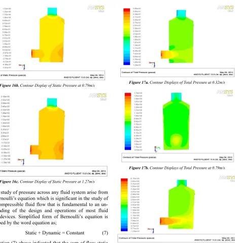
(5)The ANSYS Fluent [15] uses pressure gauge to measure the static pressure which is also the scrubber systems pres-sure at the inlet and outlet as shown in Figures 17a, 17b and 17c for the three velocities.
As shown above, for the 0.32m/s velocity the static gauge pressure was obtained to be 0.309pa and 0.0164 at the inlet and the outlet of the system. Also, for the 0.79m/s, the static gauge pressure was obtained to be 1.32pa and 0.00442pa at the inlet and outlet. However, a static gauge pressure of 3.16pa and 0.131pa at the inlet and outlet for the 1.27m/s was obtained. The pressure drop, ∆P for the three flows velocities was computed using the relation
) 2 ( )
1
( system system
P
P
P
=
−
∆
(6)Comparison between the dynamic similitude pressure obtained from the recommended pressure drop for spray tower scrubber and the computed pressure drop from the CFD analysis shown in Table 2 indicated a closer agree-ment between the two.
Table 2. Comparison between the Recommended and Computed Pressure Drop
Gas Velocity (m/s)
Recommended Pressure Drop
(pa)
Computed Pressure Drop using CFD
(pa)
0.32 0.47 0.30
0.79 1.7 1.32
1.27 2.93 3.03
Figure 16b. Contour Display of Static Pressure at 0.79m/s
Figure 16c. Contour Display of Static Pressure at 1.27m/s
The study of pressure across any fluid system arise from the Bernoulli’s equation which is significant in the study of an incompressible fluid flow that is fundamental to an un-derstanding of the design and operations of most fluid based devices. Simplified form of Bernoulli’s equation is described by the word equation as;
Static + Dynamic = Constant (7)
Equation (7) above indicated that the sum of flow static and dynamic pressure is constant along a streamline of flu-id flow.
According to [20], the sum of these two pressures is termed as the total pressure. Figures 18a, 18b and 18c shows total pressure contours for the three velocities. For 0.32m/s velocity which is the velocity at which the scrub-ber performed optimally in the simulation analysis, the total pressure is almost constant across the spray chamber. But the pressure is higher across the inlet and slightly lower along the exit. For 0.79 and 1.27m/s velocities, the total pressure is slightly higher and approximately constant within the chamber. This indicated that the proposed scrubber has conformed to the Bernoulli’s equation espe-cially at velocity of 0.32m/s. Total Pressure at 0.32m/s 1.27m/s
Figure 17a. Contour Displays of Total Pressure at 0.32m/s
Figure 17b. Contour Displays of Total Pressure at 0.79m/s
Figure 17c. Contour Displays of Total Pressure at 1.27m/s
4. Conclusion
par-ametric analysis conducted, it can be concluded that the numerical simulation using Ansys Fluent CFD is an effec-tive method of studying the flow characteristics of a coun-ter-flow wet scrubber system.
References
[1] Frank, R. S. and Nancy, W. E. 2005. Environmental Engi-neers Mathematics Handbook, CRC Press, Florid, USA, pp. 208-249.
[2] United States Environmental Protection Agency (USEPA) and National Association of Clean Air Agencies (NACAA). 2012. Control of Particulate Matter Emissions. APTI 413 Module 8 Student Manual, 39-40. Online: (www.epa.gov/apti/Materials/APTI413student/413StudentM anual/SM_ch8.pdf).
[3] Hudson Product Corporation. 2011. Air Cooled Heat Ex-changer Modeling with CFD.
[4] Kennedy, C., Diwakar, P., Leonad, J.R. and Rosendall, B. 2011. Computation Based Engineering of Multiphase Pro-cess Using CFD, Bechtel Technology Journal, vol. 3, No. 1.
[5] Minghua, B., Qiufang W. and Yu, Z. 2010. Numerical Sim-ulations of Dust Removal Device for Quicklime Slacking, Environmental and Chemical Engineering College, Yanshan University.
[6] Goniva C., Pirker, S., Tukovoc, Z., Feilmayr, C. and Burgler, T. 2009. Simulation of Off-Gas Scrubbing by a Comgined Eulerian-Lagrangian Model, 7th International Conference on CFD in the Minerals and Processing Industries, Melbourne, Australia.
[7] Caiting L., Shanhong L., Guangming, Z., Fei W., Dayong W., Hongliang, G. And Wei G. 2008. Airflow Simulation of an Umbrella Plate Scrubber, IEEE Conference Publications, The 2nd Conference on Bioinformatics and Biomedical Engi-neering, (ICBBE-2008), Shanghai, China.
[8] Shan-hong L., Cai-ting L, Guang-ming Z., Si-min L., Fei W. and Da-yong W. 2008. CFD Simulation on Performance of New type Umbrella Plate Scrubber, Transactions of Nonfer-rous Metals Society of China, vol. 18, pp 488-492.
[9] Dudek, S .A., Rogers, J. A. and Gohara, W. E. 1999. Com-putational Fluid Dynamics (CFD) Model for Predicting a Two-Phase Flow in Flue Gas Desulfurization Wet Scrubber,
EPRI-DOE-EPA Combined Utility in Air Pollution Control Symposium, Atlanta, Georgia, USA.
[10] Ashaka Cement plc., Gombe State, Nigeria. 2011.
[11] Karthik, T. S. D. 2011. Turbulence Models and their Appli-cations, Department of Mechanical Engineering, Indian In-stitute of Technology, Madras, India.
[12] Hendawi, M., Molle B. And Folton C. 2005. Measurement Accuracy Analysis of Sprinkler Irrigation Rainfall in Rela-tion to Collector Shape, Journal of IrrigaRela-tion and Drainage Engineering, vol. 131, no. 5, pp. 477-483.
[13] Lee, C. W., Palma, P. C. and Simmons, K. 2005. Compari-son of Computational Image Velocimetry Data for the Air-flow in an Aero-engine Bearing Chamber, Journal of Engi-neering for Gas Turbines and Power, vol. 127, no. 4, pp. 697-703.
[14] Xiang, R. B. And Lee, K. W. 2005. Numerical Study of Flow Field in Cyclones of Different Height, Journal of Chemical Engineering Process, vol. 44, no. 8, pp. 877-883. ANSYS Fluent 13.0 Inc., 2010. USA.
[15] United States Environmental Protection Agency (USEPA) and the National Association of Clean Air Agencies (NACAA). 2010. APTI: 4 1 3 Control of Particulate Matter Emissions , 5th Edition, Chapter 10 Student Manual. Online: (http://www.epa.gov/apti/Materials/APTI%20413%20studen t/413%20Student%20Manual/SM_ch%2010.pdf).
[16] Ngala, G. M. Sulaiman, A. I. and Sani, M. U. 2008. Air Pollution Control in Cement Factory Using Horizontal Type Wet Scrubber, Continental Journal of Applied Sciences, vol. 3, No. 1.
[17] Garba, M. N. 2005. Gas Particle Separation Using Wet Scrubber Method, M.Eng Thesis, Department of Mechanical Engineering, Bayero University Kano, Nigeria.
[18] ANSYS Fluent 12.0 Inc., 2009. USA.
[19] Yunus A. C. and John M. C. 2006. Fluid Mechanics: Fun-damentals and Applications, International Edition, McGraw Hill Publication, pp.185-201.
[20] Munson, B. R., Young, D. F., Okishi, T. H. and Huebsch. 2010. Fundamentals of Fluid Mechanics, Sixth Edition, John Wiley and Sons, pp. 332-374.
[21] Engireering ToolBox, 2013. Online: