Published online February 2, 2015 (http://www.sciencepublishinggroup.com/j/ijepe) doi: 10.11648/j.ijepe.20150401.14
ISSN: 2326-957X (Print); ISSN: 2326-960X (Online)
Open source software based modeling of MEPE test system
for stability studies
Kyaw Myo Lin
1, *, Wunna Swe
2, Pyone Lai Swe
11
Power System Research Unit, Department of Electrical Power Engineering, Mandalay Technological University, Mandalay, Myanmar
2
Power System Research Unit, Technological University of Monywa, Sagaing Region, Myanmar
Email address:
[email protected] (K. M. Lin), [email protected] (W. Swe), [email protected] (P. L. Swe)
To cite this article:
Kyaw Myo Lin, Wunna Swe, Pyone Lai Swe. Open Source Software Based Modeling of MEPE Test System for Stability Studies. International Journal of Energy and Power Engineering. Vol. 4, No. 1, 2015, pp. 23-31. doi: 10.11648/j.ijepe.20150401.14
Abstract:
This paper presents an implementation of MEPE test system in Power System Analysis Toolbox (PSAT)—free and open source software. This paper mainly focuses on the application of newly developed hydro turbine and governor model with detailed dynamic power system models on Myanmar national grid because the power system network is largely supplied by hydro power. This paper also demonstrates the rotor angle stability analysis of test system including classical small signal stability and transient stability criteria. Transient stability assessments of national grid test system are carried out through nonlinear time domain simulation by applying both large and small disturbances. Moreover, a statistical t-test is performed to ensure the effective of proposed model to deal with dynamic problem of the power system.Keywords:
Power System Modeling, MEPE Test System, Small Signal Stability, Transient Stability1. Introduction
The power system stability is defined as that property of a power system that enables it to remain in a state of operating equilibrium under normal operating conditions and to regain an acceptable state of equilibrium after being subjected to a disturbance [1]. Stability of a power system is dependent on the set of parameters describing the dynamic properties of each of its elements. Of particular importance are those parameters belonging to machines, e.g., generators, turbines, and/or governors. They play a major role in rotor angle stability which is classified into two types: small signal stability and transient stability [1]. These two types of stability are widely and intensively employed for stability security assessment at network control centers and for planning purposes.
In power system stability studies, the term transient stability usually refers to the ability of the synchronous machines to remain in synchronism during the brief period following large disturbances, such as severe lightning strikes, loss of heavily loaded transmission lines, and loss of generation stations or short circuits on buses [2]. To correct forecast dynamic responses and assess system stability, accurate modeling of power systems is highly important. The system model should be capable of
representing the behavior of the real system as close as possible. Incomplete modeling may lead to incorrect simulation results, which could in turn result in costly consequences in operation.
The Myanmar electricity network is largely supplied by hydro power while supplying large consumption in the YESB area and central region through weak transmission lines. Hydro power in Myanmar accounts for more than three-quarter (about 76%) of net production of electric generation [3]. In hydro power production systems, the functions of hydro turbine and governors cannot be neglected because they participate in primary frequency control of power system [4]. Features of hydro generators are substantially different from those of thermal generators, and their respective modeling needs to be done appropriately [5].
these facts are already implemented in industrialized commercial software. High cost, license restrictions, and limited freedom of core software modifications are the hurdles of the type of proprietary software.
Moreover, none of free and open source software (FOSS) alternatives has been utilized for the modeling of MEPE power system. The previous studies on national grid [7] are just only based on power system models developed in POWER Toolboxes [8], which was developed by Prof. Hadi Saadat. Science the toolbox doesn’t cover the dynamic modeling of detailed power system, only classical models were being utilized in step-by-step numerical simulation of transient stability assessment to get the critical clearing time (CCT) [9]. And then, the previous one was out of area on small signal stability study because of lack of dynamic system models. Moreover, none of free and open source software (FOSS) alternatives has been utilized for the modeling of MEPE test system. Hence, an alternative would be to utilize free and open source power system software that that encompasses both transient and small signal models.
In this paper, power system dynamic models of MEPE test system are developed using Power System Analysis Toolbox (PSAT) – free and open source software. PSAT [10] is an educational open source software for power system analysis study [11]. The toolbox covers fundamental and necessary routines for power system studies such as power flow, small signal stability analysis and time domain simulation. PSAT is suitable candidate as power system analysis software which is capable of performing core stability analyzes.
The main objective of this paper is to conduct research on the dynamic modeling, simulation and assessment long-term power system dynamics of MEPE grid using detailed dynamic power system models in PSAT. The study model includes a newly developed hydro turbine and hydro governor model [5] which is capable of representing the actual dynamic behavior of hydro units.
The rest of the paper is organized as follows. Section 2 expresses the test system characteristics and dynamic modeling. Simulation and results with two different hydro turbine models of MEPE test system are presented and discussed in section 3 and 4, for small signal stability and for transient stability studies, respectively. Finally, conclusions are drawn in section 5.
2. MEPE Test System
Myanmar has in installed capacity of approximately
3,460 MW of energy generation, which is composed primary of 2,660 MW (about 76%) of hydro capacity, 550 MW (about 16 %) of gas-fired capacity, 165 MW (about 5%) of steam capacity and 120 MW (3.5%) of coal-fired capacity [12, 13]. Currently, the total installed capacity of the hydropower plants is 2,660 MW with a firm capacity of 1,504 MW, out of which 860 MW is in reservoir-based plants and the rest in run-of plants. Hydro account for about 76 percent of installed capacity and 65 percent of electricity production [12]. The system analyzed in this study is a conceptualization of MEPE grid circa 2014. It is based on a system data proposed by KEPCO (MEPE consultant) and the staffs of power system department of MEPE.
2.1. System Characteristics
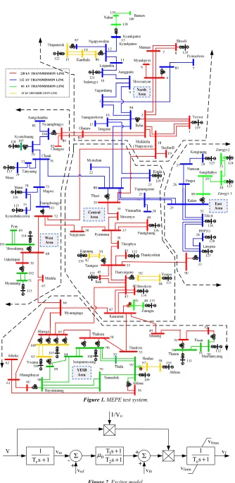
The system under study, MEPE test system is depicted in Fig. 1. The voltage levels of test system are 230 kV, 132 kV, 66 kV, and 33 kV respectively. The grid has no direct connections to other grids of neighboring countries. The five areas of MEPE test system are:
1)“West” with two hydro stations and four thermal generations and some loads,
2)“North” with four hydro units and some loads,
3)“East” with only one coal-fired station and five hydro stations and some loads,
4)“Central” with much loads and eight hydro units, and 5)“YESB” with heavy loads and seven thermal stations.
2.2. Dynamic Modeling
Dynamic models of synchronous generators, exciters, turbines, and governors for MEPE power system are implemented in PSAT. All models used are documented in the PSAT manual.
2.2.1. Generator Models
Two synchronous machine models are used in the system: three rotor windings for the salient-pole machines of hydro power plants and four rotor windings for the round-rotor machines of thermal plants. These two types of generators are described by five and six state variables, respectively. All generators have no mechanical damping and saturation effects are neglected.
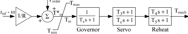
2.2.2. Automatic Voltage Regulator Models
Figure 1. MEPE test system.
Figure 2. Exciter model.
1 s T
1
r + Ts 1
1
e +
1 s T
1 s T
2 1
0 +
+
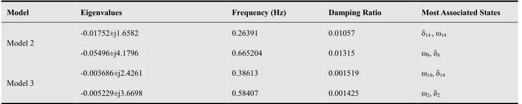
2.2.3. Turbine and Governor Models
In PSAT, there are three models of turbine and governors: namely Model 1, Model 2 and Model 3. The first one is a thermal generator model while the second is a simplified
model. As such, the system’s hydro generator is temporarily represented by Model 2 while that of thermal is represented by Model 1. Block diagrams of these two models are depicted in Fig. 3 and Fig. 4, respectively.
Figure 3. Turbine governor model used of thermal generator: Model 1.
Figure 4. Turbine governor model for simple hydro generator: Model 2.
W. Li et al. recently developed hydro turbine and governor models in PSAT [5]. The block diagram of Model 3 is shown in Fig. 5. Hydro turbine and governor are normally combined
together for representation. The block consists of a typical hydro turbine governor and a linearized hydro turbine model where the corresponding elements are depicted in Fig. 5.
Figure 5. Turbine and governor model used for typical hydro generator: Model 3.
The linearized turbine is the classical hydro turbine model in power system stability analysis, corresponding to ideal turbine and inelastic penstock with water inertial effect considered. For these models, limits of mechanical torque are checked at the initialization step. It can be also observed those mechanical torques are limits are in p.u. with respect to the mechanical power rating.
3. Small Signal Stability Analysis
Small signal stability is defined as the ability of a power system to maintain its synchronism after being subjected to a small disturbance [2]. The small signal dynamic behavior of power systems can be determined by eigenvalues analysis, which is a well-established linear-algebra analysis method [14], if a dynamic power system model is available. In an analysis of the system stability, eigenvalues of a power system
model have been derived and evaluated. Through analyzing eigenvalues, characteristics of system dynamic states are understood without a time domain simulation.
Before fulfilling eigenvalue analysis, it is necessary to calculate power flow. To conduct a load flow study, Bus No. 119 (Yeywa Station) is selected as the slack bus and other generating buses have been used as voltage controlled bus. Runge-Kutta power flow solver is applied for state variables initialization.
3.1. Eigenvalue Analysis of Test System
For linear analysis of test system, the benchmark system is implemented with Model 1 and Model 2 as well as Model 1 and Model 3. Plot of eigenvalues of test system implementing Model 2 and Model 3 are illustrated in Fig. 6 and Fig. 7, showing their respective local enlargement.
1 s T
1 s T
5 4
+ +
1 s T
1 s T
c 3
+ + 1
s T
1
s +
1 s T
1 s T
2 1
+ +
s T 1
K
p 1
+ s
K2
s T 1
s δT
r r
+
s T a 1
s )T a a a (a a
w 11
w 23 11 21 13 23
Figure 6. Eigenvalues of MEPE test system with Model 2.
The system has 315 states with Model 2 while 372 states with Model 3; the number corresponds to the same number of eigenvalues. The small signal stability analysis has been carried out for the benchmark system and all eigenvalues for the MEPE system, either with Model 2 or with Model 3, are located in the left half plane, which indicates systems are stable. It can be seen from the figures that all eigenvalues have negative real part so that the system is said to be inherently dynamically stable. Comparing the figures, it can be observed that there are more eigenvalues have lower damping ratios in the system with Model 3 than that with Model 2.
Figure 7. Eigenvalues of MEPE test system with Model 3.
For the system with Model 3, there are six paired complex eigenvalues located outside the 10% damping line. For the system with Model 3, there are twelve paired complex eigenvalues located outside the 10% damping line because of Model 2 doesn’t compose of nonlinear dynamic and only represents simple and classical model.
Table 1 provides the two lowest damping modes, their corresponding frequencies and damping ratios and the most associated state variables for both scenarios; corresponding the case with Model 2 and the case with Model 3.
Table 1. Linear analysis results of the two lowest damping modes.
Model Eigenvalues Frequency (Hz) Damping Ratio Most Associated States
Model 2
-0.01752±j1.6582 0.26391 0.01057 δ14 , ω14
-0.05496±j4.1796 0.665204 0.01315 ω8, δ8
Model 3
-0.003686±j2.4261 0.38613 0.001519 ω14, δ14
-0.005229±j3.6698 0.58407 0.001425 ω2, δ2
3.2. Mode Shades of Test System
The interarea modes are named so because in these modes, the participating machines divide into two groups, and the two groups oscillate against each other. If the interarea modes are poorly damped, or unstable, then the two groups may lose synchronism completely and this leads to system breakdown. The phenomenon of all the machines dividing into two groups may be better understood by the help of mode shapes. Mode shapes are the polar plots of the eigenvectors of a mode corresponding to the desired states. Modes shapes, or the right eigenvectors, give an insight into the relative activity of state variables in each mode.
They are obtained from the right eigenvectors, vi, in the
following equation;
r r
i i i
Av =λv (1)
The larger the magnitude of the element in r i
v , the more observable of that state variable is. In this research, the state variable, generator speed (ωi), is used for analysis. Mode
shape plots of generator speed of the corresponding case studies in Table 1 are illustrated in Fig. 8 and Fig. 9, respectively.
In all the cases, the two groups of machines oscillating against each other can easily be observed. The division of machines into opposing groups is evident in both the cases. In all figures above, the two largest magnitudes of the mode shape elements represents the generator speed: ω14 and ω2.
These two larger magnitudes are pointing out the most observable state variables.
It can be observed that ω14 is the most observable in Mode 1
of both models whereas ω8 is the most observable in Mode 3
of first case and ω2 for the later. These observations will later
be useful in input signal selection for damping control design.
-30 -20 -10 0
-20 -10 0 10 20
Real
Im
a
g
5% damping line
1% damping line 0% damping line 10% damping line
-50 -40 -30 -20 -10 0
-60 -40 -20 0 20 40 60
Real
Im
a
g
10% damping line 5% damping line
(a) Mode 1: 0.23691 Hz
(b) Mode 3: 0.665204 Hz
Figure 8. Mode shape of test system implementing Model 2.
(a) Mode 1: 0.38613 Hz
(b) Mode 3: 0.58407 Hz
Figure 9. Mode shape of test system implementing Model 3.
4. Transient Stability Analysis
Transient stability of an electrical power system refers to the ability of the system to settle at the stable equilibrium point in the post-fault system subsequent to a specific fault scenario. This stability problem can be studied either as a system stability or a structural stability problem.
4.1. Time Domain Simulation Study with Existing and Developed Models
To evaluate the transient stability of the MEPE test system, a three phase fault is applied at Bus No.22 (Myinchan Station) at t=5 s and removed at t=5.02 s. The reason why the fault is set on this bus is to decrease the fault influence on critical generators, and the same time so that the dominant power flow is not disturbed. This allows for a good comparison of the performance of the turbine and governor models implemented in MEPE test system of this article. This allows for a good comparison of the performance of the turbine and governor models implemented in MEPE benchmark system of this research.
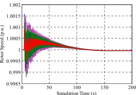
In the MEPE benchmark system, thermal turbine and governors for the 13 thermal generating stations are modeled as Model 1 while the rest hydro turbine and governors will take use of Model 2 or Model 3, respectively. Fig. 10 and 11 depict the response of the generators rotor speeds in the MEPE benchmark system with Model 2 and Model 3, respectively.
Figure 10. Response of test system with Model 2.
Figure 11. Response of test system with Model 3.
2.5e-05 5e-05
30
210
60
240 90
270 120
300 150
330
180 0
2e-05 4e-05
30
210
60
240 90
270 120
300 150
330
180 0
1e-05 2e-05
3e-05
30
210
60
240 90
270 120
300 150
330
180 0
0.0001 0.0002
0.0003 0.0004
30
210
60
240
90
270 120
300 150
330
180 0
0 50 100 150 200
0.996 0.998 1 1.002 1.004 1.006 1.008
Simulation Time (s)
R
o
to
r
S
p
e
e
d
(
p
.u
)
0 50 100 150 200
0.9985 0.999 0.9995 1 1.0005 1.001 1.0015 1.002
Simulation Time (s)
R
o
to
r
S
p
e
e
d
(
p
.u
Comparing these two simulation results, it can be easily found out that the system with Model 2 recovers to steady state faster than that with Model 3. It is because Model 2 doesn’t compose of nonlinear dynamic and only represents simple and classical model. Since Model 3 represents detail dynamic model of hydro turbine and governor, the system oscillates around the steady state than with Model 2. Moreover, in the system with Model 3, there are particular frequencies around a steady value, “1”, even when the system already gets back to steady state. In fact, this is a normal and common phenomenon in large power system called system oscillations. It is system internal swing resulting from electric power flowing from one area to another in order to keep the balance of consumption and generation.
The state of this type of oscillation was conducted in many literatures. From that comparison, it can be recommended that Model 3 represents the characteristics of hydro turbine and governor although there are some assumptions in modeling. Therefore, using Model 3 is suitable for modeling of Myanmar electric power system.
4.2. Transient Stability Assessment of Test System
To evaluate the Transient Stability Assessment (TSA) of national grid test system, recently faulted lines and stations are considered as scenarios. The major breakdown happened recently at Belin Substation (Bus2) on September 12, 2014. This breakdown is considered as the three-phase fault disturbance and time domain simulation is done.
Moreover, to demonstrate the one line tripping of double circuit line, the three-phase fault is considered at Bus 88 (Thazi Station) and breaker opening is set up on one line of Thazi-Yepaungsone 132 kV double circuit transmission line. And also, the tie-line openings set up are observed to analysis the effect of tie-line power flow on transient stability assessment. As space is limited, the simulation results of all scenarios are not illustrated.
For the deadly three-phase fault short circuit at Belin Substation compound (which happened on second week of September, 2014) due to GCB blow-out, the fault must be cleared before loss of synchronism. This situation is demonstrated in Fig. 12 and 13, respectively.
Figure 12. Unstable conditions of rotor speed oscillations due to fault at
Belin Substation.
The time-dial settings of breakers installed at the stations connected to Belin are more than 2 s. Moreover, the maximum current limits between the stations were not confirmed for control process. Therefore, there was no line tripping during the faulted time and the overall system loosed synchronism.
Figure 13. Plot of unstable voltage profile due to fault at Belin Substation.
Figure 14. Stable swings of rotor speed due to fault at Belin Substation.
According to time domain simulation with developed models, considering line tripping of Belin-Thapyaywa (heavy loaded line), the CCT is 0.11264 s. Thus, the breaker set up must be restored according to the results.
Figure 15. Plot of voltage profile for stable condition after fault clearing at
Belin Station.
0 0.5 1 1.5 2
0.7 0.8 0.9 1 1.1 1.2
Simulation Time (s)
R o to r S p e e d ( ra d /s /3 1 4 .1 5 )
Unstabe Oscillations of Generator Rotor Speed due to Fault at Bus #2
0 1 2 3 4 5 6
0 0.2 0.4 0.6 0.8 1 1.2 1.4
Simulation Time (s)
V o lt a g e M a g n it u d e ( p .u .)
Bus Voltage Oscillation due to Fault at Bus#2
Unstable Condition of Bus Voltages due to No Line Trip
0 5 10 15
0.985 0.99 0.995 1 1.005 1.01 1.015
Simulation Time (s)
R o to r S p e e d ( ra d /s /3 1 4 .1 5 )
Rotor Speed Oscillation due to Fault at Bus#2
0 1 2 3 4 5
0 0.2 0.4 0.6 0.8 1 1.2
Simulation Time (s)
V o lt a g e M a g n it u e ( p .u .)
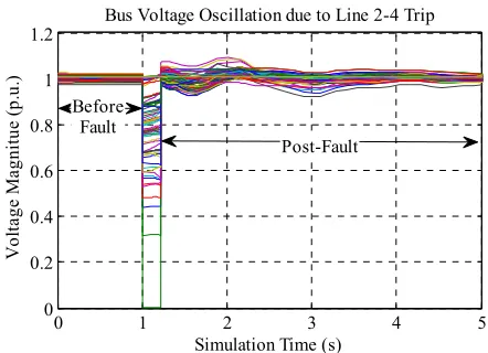
Bus Voltage Oscillation due to Line 2-4 Trip
Post-Fault Before
The following table, Table 2, summarizes the TSA on MEPE test gird in PSAT. Since maintaining synchronism between various parts of such power systems increasingly difficult and instability has disturbing effects on power system
parameters, the power system should be designed and operated so that the instability is improbable and will occur only rarely by applying various effective improving methods.
Table 2. Summary of Transient Stability Assessment.
Faulted Bus Opening Line Fault Clearing Time (sec) Critical Clearing Time (sec) TSA
2 2-18 0.11262
0.11264 Stable
2 2-18 0.11265 Unstable
9 9-82 0.15852
0.15853 Stable
9 9-82 0.15855 Unstable
23 23-88(1) 0.24910
0.24915 Stable
23 23-88(1) 0.24920 Unstable
47 47-53 0.20040
0.20045 Stable
47 47-53 0.20050 Unstable
66 66-47 0.19978
0.19995 Stable
66 66-47 0.20001 Unstable
76 76-88 0.120045
0.12006 Stable
76 76-88 0.12007 Unstable
85 85-3 0.10118
0.10119 Stable
85 85-3 0.10120 Unstable
88 88-76 0.21164
0.21165 Stable
88 88-76 0.21165 Unstable
104 104-79 0.21178
0.21186 Stable
104 104-79 0.22011 Unstable
To confirm about the newly developed model, statistical t-test is applied between two systems (with Model 2 as well as with Model 3) responses to the faults. The following section will explain about this test.
4.3. Statistical t-Test for Transient Stability Assessment
In this section, the statistical t-test is applied to evaluate the effectiveness of the developed models. The procedure of implementing t-test is not described because it can be easily observed in many literatures. Therefore, proposed hypothesis and observed results will be discussed. To prove with t-test, two samples (or treatments) are required. The data input for
t-test are the critical clearing time (CCT) of test system. The two scenarios are also considered with different fault locations. With the provision of time domain simulation with Trapezoidal rule, the CCT of two scenarios with same faulted buses are selected and used as two data set inputs for t-test.
This test decides that “Is there a specific difference between two scenarios or not?” Since the effective CCT of test systems are analyzing, a suitable null hypothesis would be that there is no difference in CCT between the two scenarios.
Let the null hypothesis: H0 = −µ1 µ2 =0.
Let the alternative hypothesis: H1= −µ1 µ2 >0.
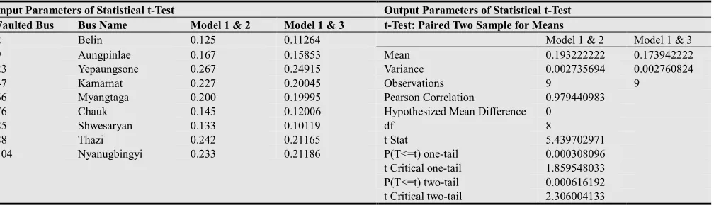
Table 3. Input and output parameters of statistical t-test.
Input Parameters of Statistical t-Test Output Parameters of Statistical t-Test Faulted Bus Bus Name Model 1 & 2 Model 1 & 3 t-Test: Paired Two Sample for Means
2 Belin 0.125 0.11264 Model 1 & 2 Model 1 & 3
9 Aungpinlae 0.167 0.15853 Mean 0.193222222 0.173942222
23 Yepaungsone 0.267 0.24915 Variance 0.002735694 0.002760824
47 Kamarnat 0.227 0.20045 Observations 9 9
66 Myangtaga 0.200 0.19995 Pearson Correlation 0.979440983
76 Chauk 0.145 0.12006 Hypothesized Mean Difference 0
85 Shwesaryan 0.133 0.10119 df 8
88 Thazi 0.242 0.21165 t Stat 5.439702971
104 Nyanugbingyi 0.233 0.21186 P(T<=t) one-tail 0.000308096
t Critical one-tail 1.859548033
P(T<=t) two-tail 0.000616192
t Critical two-tail 2.306004133
The problem requests a 5% level of significance which equates to a 95% level of certainty. Therefore, the significance level α=0.05 is established for 95% confidence interval. In the result table, the values of the mean (µ) of each data sample, the variance ( 2
d
S ), the number of observations (n), the null hypothesis (that there is no difference between the population means), the degree of freedom (df), the calculated t value (t
For most purposes, it should be used a two-tailed test rather than one-tailed test. According to the two-tailed test, the probability of getting calculated t value by chance alone is shown. That probability is extremely low, so the means are significantly different. The means for the CCT are significantly different at p = 6.1619 x 10⁻⁴. In other words, there is a probability of about 3 in 5, 000 that it would be get the observed difference between the means by chance alone. So, it can be reasonably confident that the mean CCT for test system using newly developed models is less than those using the existing models. The result decides to reject the null hypothesis, H0.
Therefore, one can conclude from this test that there is a significant moral difference between the two models. For the real case power system, the breaker must be tripped within a short duration of fault clearing time. By using the newly developed model, it can be predicted the CCT of test system more precisely than by using simple model.
5. Conclusion
This paper presents the Myanmar National grid model of which the novelty being its implementation in a free and open source software; namely Power System Analysis Toolbox (PSAT). The model takes into account detailed modeling of the dynamics which play an important role in the assessment of the system’s behavior. Of particular significance is the implementation of the recently developed hydro turbine and governor model in PSAT with the MEPE test system since more than three quarters of the national grid electric generating stations are hydro power plants.
To demonstrate the importance of accurate modeling, rotor angle stability analyses (small signal stability as well as transient stability) of the MEPE test grid model modeling with hydro turbine and governor models compared with the test system employing the existing models in PSAT.
The results highlight the importance of detailed modeling in real case off-line power system analysis using free and open source software.
Acknowledgements
The first author would like to thank to his teachers and colleagues from MTU for their support and understanding during this research. The first author would like to express his sincere thanks to his teachers for guiding him to do the research on the right track, both on practical and scientific manners. The authors greatly express sincere thanks to all persons whom will concern to support in preparing this research article and for their technical feedback on important
issues. The authors wish to express sincere appreciation to the faculty and staffs of MEPE for providing the required data and information. Last but not least, the authors gratefully acknowledge the aid of Prof. Dr. Federico Milano of School of Electrical, Electronic and Communications Engineering, University College Dublin for providing PSAT as a FOSS to the power engineering community.
References
[1] P. Kundur, Power System Stability and Control, The ERPI Power System Engineering Series, 1994, pp.17.
[2] P. Kundur, J. Paserba, V. Ajjarapu, A. Anderson, C. Canizares, N. Hatziargyriou, D. Hill, C. Taylor, T. V. Cutsem, “Definition and classification of power system stability – IEEE/CIGRE joint task force on stability terms and definition,” IEEE Trans Power Syst., vol.19, no.3, pp. 1387-1401, 2004.
[3] Myint Aung, Present and Future Power Sector Development in Myanmar, MEPE, Nay Pyi Taw, 2012.
[4] J. Machowski, J. W. Bialek, J. R. Bumby, Power System Dynamics (Stability and Control) 2nd ed., Wiley, 2008. [5] W. Li, L. Vanfretti, Y. Chompoobutrgool, “Development and
implementation of hydro turbine and governor models in a free and open source software package, Int. J. Simulation Modelling Practice and Theory, vol. 24, pp. 84-102, 2012.
[6] B. B. Sharp, D. B. Sharp, Water Hammer: Practical Solutions, Butterworth-Heinmann, 1998.
[7] K. M. Lin, W. Swe and P. L. Swe, “Computer-aided transient stability analysis of multi-machine power system,” Proceedings of WASET09, vol. 56 (B), pp. 140-144, August, 2009.
[8] H. Saadat, Power System Analysis, 4th ed., McGraw-Hill, Singapore, 2004.
[9] K. M. Lin, “ Computer Aided Transient Stability Analysis of Myanmar Electric Power System,” WYTU, Yangon, 2010. [10] F. Milano, PSAT, Matlab-based Power System Analysis
Toolbox, 2009.
(http://www.power.uwaterloo.ca/∼fmilano/downloads.html) [11] F. Milano, “An Open Source Power System Analysis Toolbox,”
IEEE Trans Power Syst., vol. 20, no.3, pp. 1199-1206, 2005. [12] Kyaw Swar Soe Naing, “Fuel mix requirements for power
generation in Myanmar,” MEPE, Nay Pyi Taw, 2013.
[13] Asia Development Bank, Energy Sector Initial Assessment Myanmar, 2013.