The global dynamical complexity of the human brain network

R E S E A R C H

Open Access

The global dynamical complexity of the

human brain network

Xerxes D. Arsiwalla

and Paul F. M. J. Verschure

*Correspondence: [email protected] 1_{Synthetic Perceptive Emotive and} Cognitive Systems (SPECS) Lab, Center of Autonomous Systems and Neurorobotics, Universitat Pompeu Fabra, Barcelona, Spain Full list of author information is available at the end of the article

Abstract

How much information do large brain networks integrate as a whole over the sum of their parts? Can the dynamical complexity of such networks be globally quantified in an information-theoretic way and be meaningfully coupled to brain function? Recently, measures of dynamical complexity such as integrated information have been proposed. However, problems related to the normalization and Bell number of partitions

associated to these measures make these approaches computationally infeasible for large-scale brain networks. Our goal in this work is to address this problem. Our formulation of network integrated information is based on the Kullback-Leibler divergence between the multivariate distribution on the set of network states versus the corresponding factorized distribution over its parts. We find that implementing the maximum information partition optimizes computations. These methods are

well-suited for large networks with linear stochastic dynamics. We compute the integrated information for both, the system’s attractor states, as well as non-stationary dynamical states of the network. We then apply this formalism to brain networks to compute the integrated information for the human brain’s connectome. Compared to a randomly re-wired network, we find that the specific topology of the brain generates greater information complexity.

Keywords: Brain networks, Neural dynamics, Complexity measures

Introduction

From a computational neuroscience perspective, the brain is oftentimes abstracted as a complex information processing network, that integrates sensory inputs from multi-ple modalities in order to generate action and cognition. In this paper, we ask a much simpler question: viewing the brain as a dynamical network of neural masses, how can one compute the information integrated by such networks in the course of dynamical transitions from one state to another? A possible approach, among others, is to look at information-theoretic complexity measures that seek to quantify information generated by all causal sub-processes in such a network. One candidate measure for global dynam-ical complexity is integrated information, usually denoted as. It was first introduced in neuroscience as a complexity measure for neural networks, and by extension, as a pos-sible correlate of consciousness itself (Tononi et al. 1994). It is defined as the quantity of information generated by a network as a whole, due to its causal dynamical interac-tions, and one that is over and above the information generated independently by the disjoint sum of its parts. As a complexity measure,seeks to operationalize the intuition

that complexity arises from simultaneous integration and differentiation of the network’s structural and dynamical properties. As such, the interplay of integration and differen-tiation in a network’s dynamics is hypothesized to generate information that is highly diversified yet integrated, thereby creating patterns of high complexity. The aim of this paper is to develop mathematical tools for computing integrated information (analytically when possible, otherwise numerically) for large networks. We then apply this framework to the large-scale structural connectivity network of the human brain.

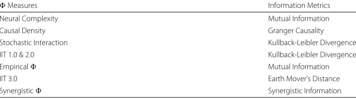
Let us begin with a brief review of the rich history of this field. The earliest propos-als defining integrated information were made in the pioneering work of (Tononi 2004; Tononi and Sporns 2003; Tononi et al. 1994). Since then, considerable progress has been made towards development of a normative theory as well as applications of integrated information (Arsiwalla and Verschure 2013; 2016a; Balduzzi and Tononi 2008; 2009; Barrett and Seth 2011; Krohn and Ostwald 2016; Mediano et al. 2016; Oizumi et al. 2014; Tononi 2012). Similar information-based approaches have also been successfully applied to many-body problems in other domains, such as, for the problem of estimat-ing microstates of statistical mechanical ensembles (Arsiwalla 2009). In fact, there are now several candidate measures of integrated information such as neural complexity (Tononi et al. 1994), causal density (Seth 2005),from integrated information theory: IIT 1.0, 2.0 & 3.0 (Balduzzi and Tononi 2008; Oizumi et al. 2014; Tononi 2004), stochas-tic interaction (Ay 2015; Wennekers and Ay 2005), empirical(Barrett and Seth 2011) and synergistic(Griffith 2014; Griffith and Koch 2014), plus several variations of these (see Tegmark (2016) for an overview). Table 1 summarizes these measures along with corresponding information metrics upon which they have been based.

Many of the above measures have been useful in different domains of validity. How-ever, applications to realistic data and in particular to large-scale networks have proven computationally challenging. With a focus on developing computational tools, we discuss three of the above measures in more detail. The measure of (Balduzzi and Tononi 2008) has been quite useful for discrete-state, deterministic, Markovian systems with the max-imum entropy distribution. On the other hand, the measure of (Barrett and Seth 2011) has been applied to continuous-state, stochastic, non-Markovian systems and in princi-ple, admits dynamics with any empirical distribution (although in practice, it is easier to use assuming Gaussian distributions). The formulation in (Barrett and Seth 2011) is based on mutual information, whereas (Balduzzi and Tononi 2008) uses a measure based on the Kullback-Leibler divergence. Note however, that in some cases the measure of (Barrett and Seth 2011) can take negative values and that complicates its interpreta-tion. The Kullback-Leibler based definition computes the information generated during

Table 1Candidate measures of integrated information shown alongside information metrics used in their respective formulations

Measures Information Metrics

Neural Complexity Mutual Information

Causal Density Granger Causality

Stochastic Interaction Kullback-Leibler Divergence

IIT 1.0 & 2.0 Kullback-Leibler Divergence

Empirical Mutual Information

IIT 3.0 Earth Mover’s Distance

state transitions and as we shall see remains positive in the regime of stable dynamics. This makes it easier to interpret as an integrated information measure. Both measures (Balduzzi and Tononi 2008; Barrett and Seth 2011) make use of a normalization scheme in their formulations. Normalization inadvertently introduces ambiguities in computa-tions. The normalization is actually used for the purpose of determining the partition of the network that minimizes the integrated information, but a normalization dependent choice of partition ends up influencing the value and interpretation of. An alternate measure based on the Earth Mover’s distance was proposed in (Oizumi et al. 2014). This does away with the normalization problem (though the current version is not formulated for continuous-state variables). However, the formulation of (Oizumi et al. 2014) lies out-side the scope of standard information theory and is still very difficult for performing computations on large networks.

A comment on network partitions is relevant at this point. The three measures of discussed above, make use of what is called the minimum information partition or minimum information bi-partition (MIP/MIB). The issue with this partitioning is that it leads to a combinatorial explosion in the number of configurations to be evaluated when working with networks having a large number of nodes. As a result, applica-tion of the above measures to compute integrated informaapplica-tion of very large networks remains challenging, particularly for the scale of networks obtained from neuroimaging data. On the other hand, in earlier work (Arsiwalla and Verschure 2013), we have intro-duced a formulation of integrated information that overcomes both, the normalization and combinatorial problem by using a different partitioning of the network called the maximum information partition (MaxIP), which opens the prospect of large-scale appli-cations. However, the formulation in (Arsiwalla and Verschure 2013) was only applicable for uncorrelated node dynamics, which may not be realistic enough for many biological systems.

In this paper, we seek to go beyond (Arsiwalla and Verschure 2013; 2016a; 2016b), starting with an extension of the formalism to include node correlations and also non-stationarity. In order to do that, we solve the discrete-time Lyapunov equation, the solution of which, is then used to get fully analytic expressions forwith network correla-tions. We consider networks with linear stochastic dynamics, which generate multivariate time-series signals. Furthermore, our networks are plastic, in the sense that connection weights are scalable using a global coupling parameter. We computeas a function of this coupling. We also extend our framework to include non-stationary dynamics. This gives usas a function of time, computed through the temporal evolution of the system. The stationary solution yieldsat the fixed-point attractor, whereas the non-stationary solution leads toelsewhere in the phase space of the system.

Stochastic integrated information

Mathematical formulation

We consider networks with linear stochastic dynamics. The state of each node is given by a random variable pertaining to a given probability distribution. These variables may either be discrete-valued or continuous. However, for many biological applications, Gaussian distributed, continuous-valued state variables are fairly reasonable abstractions (for example, aggregate neural population firing rate, EEG or fMRI signals). The state of the networkXtat time tis taken as a multivariate Gaussian variable with distribution

PXt(xt). xt denotes an instantiation of Xt with components xit (igoing from 1 ton, n being the number of nodes). When the network makes a transition from an initial state X0 to a stateX1 at time t = 1, observing the final state generates information about

the system’s initial state. The information generated equals the reduction in uncertainty regarding the initial stateX0. This is given by the conditional entropyH(X0|X1). In order

to extract that part of the information generated by the system as a whole, over and above that generated individually by its parts, one computes the relative conditional entropy given by the Kullback-Leibler divergence of the conditional distributionPX0|X1=x(x)of the system with respect to the joint conditional distributionsr_k=1P_Mk

0|Mk1=mof its non-overlapping sub-systems demarcated with respect to a partitionPr of the system intor distinct sub-systems. Denoting this as_Pr, we have

Pr

X0→X1=x

= DKL

PX0|X1=x

r

k=1 P_Mk

0|Mk1=m

(1)

where for anrpartitioned system, the state variableX0 can be decomposed as a direct

sum of state variables of the sub-systems

X0=M10⊕M20⊕ · · · ⊕Mr0= r

k=1

Mk0 (2)

and similarly,X1decomposes as

X1=M11⊕M21⊕ · · · ⊕Mr1= r

k=1

Mk1 (3)

For stochastic systems, it is useful to work with a measure that is independent of any specific instantiation of the final statex. So we average with respect to final states to obtain an expectation value from Eq. (1). After some algebra, we get

Pr(X0→X1)= −H(X0|X1)+

r

k=1 H

Mk0|Mk1

(4)

The state variable at each time t = 0 and t = 1 follows a multivariate Gaussian distribution

X0∼N(x¯0,(X0)) X1∼N(x¯1,(X1)) (5)

The generative model for this system is equivalent to a multi-variate auto-regressive process (Barrett et al. 2010)

X1=AX0+E1 (6)

whereAis the weighted adjacency matrix of the network andE1is Gaussian noise. Next, taking the mean and covariance respectively on both sides of this equation, while holding the residual independent of the regression variables, yields

¯

x1=Ax¯0 (X1)=A(X0)AT+(E) (7)

In the absence of any external inputs, stationary solutions of a stochastic linear dynam-ical system as in Eq. (6) are fluctuations about the origin. Therefore, we can shift coordinates to set the meansx¯0and consequentlyx¯1to the zero. The second equality in

Eq. (7) is the discrete-time Lyapunov equation and its solution will give us the covariance matrix of the state variables.

The conditional entropy for a multivariate Gaussian variable was computed in (Barrett and Seth 2011)

H(X0|X1)=

1

2nlog(2πe)− 1

2log [det(X0|X1)] (8) which is fully specified by the conditional covariance matrix. Inserting this in Eq. (4) yields

_Pr(X0→X1)=

1 2log

r

k=1det

Mk₀|Mk₁ det(X0|X1)

(9)

Now, in order to compute the conditional covariance matrix we make use of the identity (proof of this identity for the Gaussian case was demonstrated in (Barrett et al. 2010))

(X|Y)=(X)−(X,Y)(Y)−1(X,Y)T (10)

The appropriate covariance we will need to insert in this expression is

(X0,X1)≡

(X0− ¯x0) (X1− ¯x1)T

=(X0)AT (11)

which gives for the conditional covariance

(X0|X1)=(X0)−(X0)AT(X1)−1A(X0)T (12)

And similarly for the sub-systems

Mk0|Mk1

=Mk0

−Mk0

AT k

Mk1 −1

A_kMk0 T

(13)

wherekindexes the partition such thatMk₀denotes thekthsub-system att =0 andA_k denotes the restriction of the adjacency matrix to thekthsub-network.

Further, for linear multi-variate systems, a unique fixed point always exists. We try to find stable stationary solutions of the dynamical system. In that regime, the multi-variate probability distribution of states approaches stationarity and the covariance matrix converges, such that

t= 0 andt =1 refer to time-points taken after the system converges to the fixed point. Then the discrete-time Lyapunov equations can be solved iteratively for the stable covari-ance matrix (Xt). For networks with symmetric adjacency matrix and independent

Gaussian noise, the solution takes a particularly simple form

(Xt)=

1−A2−1(E) (15)

and for the parts, we have

(Mk0)=(X0)_k (16)

given by the restriction of the full covariance matrix on the kth sub-network. Note that Eq. (16) is not the same as Eq. (15) on the restricted adjacency matrix as that would mean that the sub-network has been explicitly severed from the rest of the sys-tem. Indeed, Eq. (16) is precisely the covariance of the sub-network while it is still part of the network and yields the integrated and differentiated information of the whole network that is greater than the sum of these connected parts. Inserting Eqs. (12), (13), (15) and (16) into Eq. (9) yields as a function of network weights for symmetric and correlated networks. For the case of asymmetric weights, the entries of the covariance matrix cannot be explicitly expressed as a matrix equation. How-ever, they may still be solved by Jordan decomposition of both sides of the Lyapunov equation.

The maximum information partition

Following (Arsiwalla and Verschure 2013; Edlund et al. 2011), the maximum information partition (MaxIP) is defined as the partition of the system into its irreducible parts. This is the finest partition and is unique as there is only one way to combinatorially reduce a system into all of its sub-units. This partition can directly be found by construction and does not require a normalization scheme for sampling through the space of multi-partitions in order to search for the one that either maximizes or minimizes the integrated information. Consequently, the resulting value ofcomputed using the MaxIP is free from normalization dependencies.

Moreover, the MaxIP also helps reduce computational cost. This can be seen as fol-lows. Prescriptions using the MIP/MIB are typically evaluated for a large class of network bi-partitions, whereas the MaxIP is uniquely defined. The number of bi-partitions of a set ofnelements is given by the sum of binomial coefficients[_pn/₌₁2] nCp, wherenCp = n!/p! (n−p)! withn!= n×(n−1)× · · · ×1 and [n/2] denotes the nearest integer less that or equal ton/2. Among all possible bi-partitions, MIP/MIB prescriptions usually restrict to those that divide the system into approximately equal parts. This still leaves us withnC[n/2]configurations for whichhas to be computed. Table 2 summarizes how this number scales with network size from a single node to a million nodes.

Table 2Scaling of network configurations upon computingusing the MIP/MIB versus using the MaxIP for networks withnnodes

No. of nodesn No. of equal part bi-partitions= n_C

[n/2] No. of MaxIPs= nCn

1 1 1

10 252 1

100 1.01_×1029 ₁

1000 2.70×10299 1

1000000 7.90×10301026 ₁

irreducible units, subtracting the information of a composite (when treating the compos-ite as a part) from the information of the whole system will always produce a smaller than that obtained by subtracting the information of each irreducible unit of the network from that of the whole network. Thereforecomputed using the MaxIP is the max-imum possible integrated information of the system compared tocomputed using any other partition of the network. In that sense, unlike the MIP or MIB, the MaxIP in fact captures the complete information integrated by the network and is therefore a more natural choice for quantifying whole versus parts.

Analytic solutions for

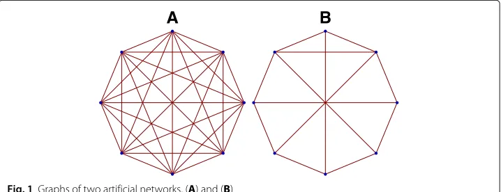
Now that we have a rigorous analytic formulation of integrated information, let us first demonstrate examples of computations performed using artificial networks. In Fig. 1 we consider two artificial networks. For these cases, we want to compute the exact analytic solution for. Each of these networks have 8 dimensional adjacency matrices with bi-directional weights (though our analysis does not depend on that and works as well with directed graphs). We want to computeas a function of network weights, which we keep as free parameters. However, in order to constrain the space of parameters, we shall set all weights to a single parameter, the global coupling strengthg. This gives usas an analytic function ofg.

for attractor states

We first computein the stationary regime, that is, when the system has converged to its fixed-point attractor state. The results for the two networks labeled a and b respectively are shown in Eqs.(17), (18) respectively. These are computed for a single time-step,

A

B

corresponding to the stable stationary solution of the system.

A = 1 2log

1−43g28

1−50g2_+49g48 (17)

B = 1 2log

B1·B2·B3·B4·B5

−1+g24_1−8g2_+4g46_1−17g2_+72g4_−64g6_+16g88 (18) where

B1 =

1−15g2+56g4−56g6+16g8

B2 =

1−15g2+54g4−54g6+16g8

B3 =

1−22g2+159g4−426g6+336g8−80g102

B4 =

1−21g2+147g4−401g6+374g8−136g10+16g122

B5 =

1−23g2+183g4−612g6+835g8−526g10+152g12−16g142 (19)

Note that the mathematical framework described above is in no way limited by the size of the network and thus, in principle, can be applied to networks of any size, to yield exact results. The only practical difficulty would be in the form of available computing hard-ware resources. Hence, for very large data networks, such as those from brain imaging, numerical computations ofwould be more practical to perform.

for non-stationary dynamics

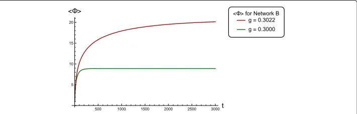
The mathematical formulation developed above can also be used to computeat non-stationary points in the solution space of networks with linear stochastic dynamics. We show this explicitly for Network B in Fig. 1. We computefor the complete tempo-ral evolution of the system starting from an initial condition att = 0 until the system stabilizes at the fixed point attractor. In the non-stationary case, Eqs. (14), (15) and (16) no longer hold. However, everything up to and including Eq. (13) are valid. Hence, the covariance matrix(Xt)is simply computed recursively following Eq. (7). Subsequently, (Xt)andare both computed for each time-pointt.

Figure 2 shows the multivariate time-series signals generated by Network B for two different coupling strengthsg. The critical value ofgfor this network is 0.3023, at which the dynamics becomes unstable. Forg ≤0.3023, the system converges to the fixed-point at the origin. In Fig. 3 we plot temporal profiles offor both the above values ofg, which shows increasing integrated information for stronger coupled networks.

Application to brain connectomics

Fig. 2Simulated time-series data for Network B following the generative model in Eq. (6). The plot on theleft shows simulated data corresponding to network coupling strengthg=0.3000 and variance of noiseσ=1. The plot on therightrefers to data from the same network with couplingg=0.3022 and the same noise amplitude. Each plot shows 8 time-series profiles, corresponding to the 8 nodes of the network (note that several of these profiles intersect or overlap with each other, hence in theaboveplots they appear to be clustered together). The time-series for each node is shown in a different color and the color scheme is the same for the plot on theleftand the one on theright. Stability of the system is guaranteed until the critical coupling atg₌0.3023. Closer to the critical point, the system takes longer to converge to the fixed-point attractor atx₌0

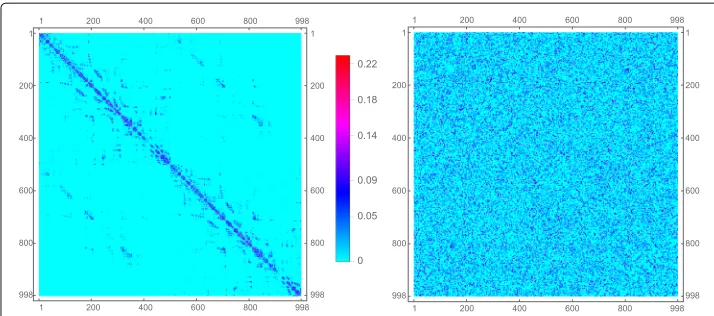
trajectories across the entire white matter. From this, connection weights between pairs of ROIs are determined, resulting in a weighted network of structural connectivity across the entire brain. We have displayed the data in matrix form as a 998 dimensional matrix on the left-hand side of Fig. 4. The 998 voxels (ROIs) represent nodes of the network. Each node is physically a population of neurons. The edges are weighted fiber counts between populations. Additionally, we include a global coupling variableg, multiplying the entire matrix, that can be used to tune the overall strength of the weights.

To simulate brain dynamics, one may chose from among a variety of possible mod-els, discussed in (Arsiwalla et al. 2013, 2015a,b; Galán 2008). To run these simulations, one may use customizable tools such as those described in (Betella et al. 2014a,b; 2013; Omedas et al. 2014). The simplest model among the ones mentioned above is the linear stochastic Wilson-Cowen model. In fact, it can be seen from (Galán 2008) that Eq. (6) is precisely a special case of the discrete-time limit of the linear stochastic Wilson-Cowen model. That is what we use here. The brain’s state of spontaneous activity or resting-state is usually identified as the attractor state of these models. This corresponds to finding

Fig. 4Left: Connectivity matrix of human cerebral white matter.Right: Randomized version of the same matrix, preserving network weights. The data consists of white matter fiber tracts from 998 cortical voxels. The connectivity matrix on theleftis a weighted matrix with thecolor-bar(in themiddle) indicating connection strengths. The randomized matrix on therightis obtained by randomly shuffling positions of weights from the connectivity matrix

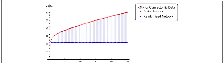
stable stationary solutions of the system. This is precisely the regime in which we com-putein bits as a function of the couplingg. The results are shown in the red profile in Fig. 5. Further, in order to contrast this result with a null model, we also rewired the edges of the connectome network randomly, while preserving the magnitude of the weights. This generates the randomized data matrix shown on the right-hand side of Fig. 4. We also compute for this matrix. The resulting profile is the blue curve in Fig. 5. For extremely small couplings, the two networks are indistinguishable onscores, how-ever, asg grows, the architecture of the brain’s network turns out to perform better at integrating information than its randomized counterpart.

While Fig. 5 depicts the fixed-point behavior ofas a function ofg, in Fig. 6 we show the full time-course offor both the connectome network as well as its randomized counterpart at a specific value of the couplingg = 1.488. The non-stationary behavior is computed using linearized dynamics as discussed above. Asymptotic values ofin Fig. 6 converge to those in Fig. 5 atg = 1.488. Once again we find that the connectomic

Fig. 6A comparison of temporal profiles offor the brain connectome network versus its randomized counterpart, both computed at a fixed couplingg=1.488. The asymptotes of these profiles match the stationary values ofin Fig. 5 for the given coupling

network completely dominates its randomized counterpart in the quantity of information it integrates and this difference only gets more pronounced upon approaching the attrac-tor state. Note that for a more thorough comparison, one might also want to check the above against an entire distribution of random networks. However, the main point of this paper is to demonstrate a systematic computation of how much information a realistic large network integrates. Functionally, what this corresponds to in terms of brain func-tion or disease is an interesting quesfunc-tion by itself. A possible approach towards addressing those issues would be to perform computations as the one demonstrated above for a large repertoire of neuroimaging studies ranging from task-based paradigms to disease states and use that to calibrate brain functional states on a scale of information complexity. Another question on which there is still no consensus concerns consciousness (Arsiwalla et al. 2016a). While it is generally agreed that information integration is a necessary com-ponent of phenomenological consciousness, by itself, it may not be sufficient (Arsiwalla et al. 2016b, Verschure 2016).

Discussion

In this paper, we have demonstrated a computational framework, built on a rich body of earlier work on information-theoretic complexity measures and applied it to compute the integrated information of large networks endowed with linear stochastic dynamics. Integrated information is interesting as a global measure of a system’s dynamical com-plexity. Whereas local complexity measures such as Granger causality, transfer entropy or synergistic mutual information have been very successful at quantifying local infor-mation processes of complex systems (Wibral et al. 2014), global measures such as integrated information serve to complement local measures and give insights on the system’s collective behavior.

neural activity on this network, we compute the integrated information of this dynamical system during state transitions for both, stationary as well as non-stationary dynamics. For the linearized system, the stationary solution corresponds to the network’s resting state attractor. The computed integrated information depends on both, the structural anatomy as well as the network’s dynamical operating point, that is, the value of the global couplingg.

We see potentially useful applications of our information-based measures for other types of physiological data as well, for example, tracing studies or detailed microscopic connectivity data. As for neuroimaging studies, information-based methods offer a useful way to quantify complexity of brain functions. The clinical utility of our measure would be in identifying information-based differences between healthy subjects and patients of neurodegenerative diseases. Just as we identified a transitionary phase after which an anatomical network strongly differs in information integration and differentiation from a randomly rewired network, similar comparative analysis for patients compared to healthy controls might provide a quantification of the extent of the disorder and even provide an analytic way to suggest diagnostic surgical rewiring to restore network processing.

Acknowledgements

This work has been supported by the European Research Council’s CDAC project: “The Role of Consciousness in Adaptive Behavior: A Combined Empirical, Computational and Robot based Approach” (ERC-2013- ADG 341196).

Authors’ contributions

All authors contributed to this work. Both authors read and approved the final manuscript.

Competing interests

The authors declare that they have no competing interests. Both authors read and approved the final manuscript.

Author details

1_{Synthetic Perceptive Emotive and Cognitive Systems (SPECS) Lab, Center of Autonomous Systems and Neurorobotics,}

Universitat Pompeu Fabra, Barcelona, Spain.2_{Institució Catalana de Recerca i Estudis Avançats (ICREA), Barcelona, Spain.}

Received: 16 July 2016 Accepted: 24 November 2016

References

Arsiwalla XD (2009) Entropy functions with 5d chern-simons terms. J High Energy Phys 2009(09):059

Arsiwalla XD, Betella A, Martínez E, Omedas P, Zucca R, Verschure P (2013) The Dynamic Connectome: a Tool for Large Scale 3D Reconstruction of Brain Activity in Real Time. In: Rekdalsbakken W, Bye R, Zhang H (eds). 27th European Conference on Modeling and Simulation. ECMS, Alesund (Norway). doi:107148/2013-0865-0869

Arsiwalla XD, Dalmazzo D, Zucca R, Betella A, Brandi S, Martinez E, Omedas P, Verschure P (2015a) Connectomics to semantomics: Addressing the brain’s big data challenge. Procedia Comput Sci 53:48–55

Arsiwalla XD, Herreros I, Moulin-Frier C, Sanchez M, Verschure PF (2016a) Is consciousness a control process? In: Nebot A, Binefa X, Lopez de Mantaras R (eds). Artificial Intelligence Research and Development. IOS Press, Amsterdam. pp 233–238. doi:10.3233/978-1-61499-696-5-233

Arsiwalla XD, Herreros I, Verschure P (2016b) On three categories of conscious machines. In: Lepora NF, Mura A, Mangan M, Verschure PF, Desmulliez M, Prescott TJ (eds). Biomimetic and Biohybrid Systems: 5th International Conference, Living Machines 2016, Edinburgh, UK, July 19–22, 2016. Proceedings. Springer International Publishing, Cham. pp 389–392. doi:10.1007/978-3-319-42417-0_35

Arsiwalla XD, Verschure PF (2013) Integrated information for large complex networks. In: The 2013 International Joint Conference on Neural Networks (IJCNN). pp 1–7. doi:10.1109/IJCNN.2013.6706794

Arsiwalla XD, Verschure P (2016a) Computing information integration in brain networks. In: Wierzbicki A, Brandes U, Schweitzer F, Pedreschi D (eds). Advances in Network Science: 12th International Conference and School, NetSci-X 2016, Wroclaw, Poland, January 11-13, 2016, Proceedings. Springer International Publishing, Cham. pp 136–146. doi:10.1007/978-3-319-28361-6_11

Arsiwalla XD, Verschure PF (2016b) High integrated information in complex networks near criticality. In: Villa AEP, Masulli P, Pons Rivero AJ (eds). Artificial Neural Networks and Machine Learning – ICANN 2016: 25th International Conference on Artificial Neural Networks, Barcelona, Spain, September 6–9, 2016, Proceedings, Part I. Springer International Publishing, Cham. pp 184–191. doi:10.1007/978-3-319-44778-0_22

Arsiwalla XD, Zucca R, Betella A, Martinez E, Dalmazzo D, Omedas P, Deco G, Verschure P (2015b) Network dynamics with brainx3: A large-scale simulation of the human brain network with real-time interaction. Front Neuroinformatics 9(2). doi:10.3389/fninf.2015.00002

Balduzzi D, Tononi G (2008) Integrated information in discrete dynamical systems: motivation and theoretical framework. PLoS Comput Biol 4(6):e1000091

Balduzzi, D, Tononi G (2009) Qualia: the geometry of integrated information. PLoS Comput Biol 5(8):e1000462 Barrett AB, Barnett L, Seth AK (2010) Multivariate granger causality and generalized variance. Phys Rev E 81(4):041907 Barrett AB, Seth AK (2011) Practical measures of integrated information for time-series data. PLoS Comput Biol

7(1):e1001052

Betella A, Bueno EM, Kongsantad W, Zucca R, Arsiwalla XD, Omedas P, Verschure PF (2014a) Understanding large network datasets through embodied interaction in virtual reality. In: Proceedings of the 2014 Virtual Reality International Conference. ACM, New York. pp 23:1–23:7. doi:10.1145/2617841.2620711

Betella, A, Cetnarski R, Zucca R, Arsiwalla XD, Martinez E, Omedas P, Mura A, Verschure PFMJ (2014b) BrainX3: embodied exploration of neural data. In: Proceedings of the 2014 Virtual Reality International Conference. ACM, Laval. pp 37:1–37:4. doi:10.1145/2617841.2620726

Betella A, Martínez E, Zucca R, Arsiwalla XD, Omedas P, Wierenga S, Mura A, Wagner J, Lingenfelser F, André E, et al (2013) Advanced interfaces to stem the data deluge in mixed reality: placing human (un) consciousness in the loop. In: ACM SIGGRAPH 2013 Posters. ACM, New York. pp 68:1–68:1. doi:10.1145/2503385.2503460

Edlund JA, Chaumont N, Hintze A, Koch C, Tononi G, Adami C (2011) Integrated information increases with fitness in the evolution of animats. PLoS Comput Biol 7(10):e1002236

Galán RF (2008) On how network architecture determines the dominant patterns of spontaneous neural activity. PLoS One 3(5):e2148

Griffith V (2014) A principled infotheoretic\phi-like measure. arXiv preprint arXiv:1401.0978

Griffith V, Koch C (2014) Quantifying synergistic mutual information. In: Prokopenko M (ed). Guided Self-Organization: Inception. Springer Berlin Heidelberg, Berlin. pp 159–190. doi:10.1007/978-3-642-53734-9_6

Hagmann P, Cammoun L, Gigandet X, Meuli R, Honey CJ, Wedeen VJ, Sporns O (2008) Mapping the Structural Core of Human Cerebral Cortex. PLoS Biol 6(7):15

Honey CJ, Sporns O, Cammoun L, Gigandet X, Thiran JP, Meuli R, Hagmann P (2009) Predicting human resting-state functional connectivity from structural connectivity. Proc Natl Acad Sci 106(6):2035–2040

Krohn S, Ostwald D (2016) Computing integrated information. arXiv preprint arXiv:1610.03627

Mediano PA, Farah JC, Shanahan M (2016) Integrated information and metastability in systems of coupled oscillators. arXiv preprint arXiv:1606.08313

Oizumi M, Albantakis L, Tononi G (2014) From the phenomenology to the mechanisms of consciousness: integrated information theory 3.0. PLoS Comput Biol 10(5):e1003588

Omedas P, Betella A, Zucca R, Arsiwalla XD, Pacheco D, Wagner J, Lingenfelser F, Andre E, Mazzei D, Lanatá A, Tognetti A, de Rossi D, Grau A, Goldhoorn A, Guerra E, Alquezar R, Sanfeliu A, Verschure PFMJ (2014) Xim-engine: a software framework to support the development of interactive applications that uses conscious and unconscious reactions in immersive mixed reality. In: Proceedings of the 2014 Virtual Reality International Conference. ACM, New York. p 26. doi:10.1145/2617841.2620714

Seth AK (2005) Causal connectivity of evolved neural networks during behavior. Netw Comput Neural Syst 16(1):35–54 Tegmark M (2016) Improved measures of integrated information. arXiv preprint arXiv:1601.02626

Tononi G (2004) An information integration theory of consciousness. BMC Neurosci 5(1):42

Tononi, G (2012) Integrated information theory of consciousness: an updated account. Arch Ital Biol 150(2-3):56–90 Tononi G, Sporns O (2003) Measuring information integration. BMC Neurosci 4(1):31

Tononi G, Sporns O, Edelman GM (1994) A measure for brain complexity: relating functional segregation and integration in the nervous system. Proc Natl Acad Sci 91(11):5033–5037

Verschure PF (2016) Synthetic consciousness: the distributed adaptive control perspective. Phil Trans R Soc B 371(1701):20150448

Wennekers T, Ay N (2005) Stochastic interaction in associative nets. Neurocomputing 65:387–392

Wibral M, Vicente R, Lizier JT (2014) Transfer entropy in neuroscience(Wibral M, Vicente R, Lizier JT, eds.). Springer Berlin Heidelberg, Berlin. doi:10.1007/978-3-642-54474-3_1

Submit your manuscript to a

journal and benefi t from:

7Convenient online submission 7Rigorous peer review

7Immediate publication on acceptance 7Open access: articles freely available online 7High visibility within the fi eld

7Retaining the copyright to your article