e-ISSN: 2278-067X, p-ISSN: 2278-800X, www.ijerd.com
Volume 11, Issue 01 (January 2015), PP.09-17
The Geometric Characteristics of the Linear Features in Close
Range Photogrammetry
Abo El-Hassan Rahil
1, Alzaed, A
21Prof. Civil Eng. Dept., College of Engineering, Taif University, KSA
Permanent Address: Civil Eng.Dept. College of Eng., Minoufiya University, Sheben El Kom, Egypt
2
Assist. Prof. Arch. Eng. Dept., College of Engineering, Taif University, KSA.
Abstract:- The accuracy of photogrammetry can be increased with better instruments, careful geometric characteristics of the system, more observations and rigorous adjustment. The main objective of this research is to develop a new mathematical model of two types of linear features (straight line, spline curve) in addition to relating linear features in object space to the image space using the Direct Linear Transformation (DLT). The second main objective of the present paper is to study of some geometric characteristics of the system, when the linear features are used in close range photogrammetric reduction processes. In this research, the accuracy improvement has been evaluated by adopting certain assessment criteria, this will be performed by computing the positional discrepancies between the photogrammetrically calculated object space coordinates of some check object points, with the original check points of the test field, in terms of their respective RMS errors values. In addition, the resulting least squares estimated covariance matrices of the check object point's space coordinates. To perform the above purposes, some experiments are performed with synthetic images. The obtained results showed significant improvements in the positional accuracy of close range photogrammetry, when starting node, end nodes, and interior node on straight line and spline curve are increased with certain specifications regarding the location and magnitude of each type of them.
Keywords:- Accuracy -linear features - geometric characteristics- close range photogrammetry.
I.
INTRODUCTIONAccording to torlegard (1981), the price for an increased accuracy has to be paid with better instruments, careful geometrical characteristics of the system, more observations and rigorous adjustment. Generally, the geometric characteristics of the system are composed of base to object distance ratio, camera axis convergence, number and disposition of the control points and number of the camera stations. In this study, the linear features will be used in the photogrammetric reduction processes. This means that the linear features (the straight line feature and the spline curve) will be used instead of the control points, to perform the photogrammetric reduction processes. One of the main objectives of the present paper is to study the effect of disposition, number of the linear features and number of points that defined the linear features.In this paper; we give short background to the linear features. Simulated cases studies will be given. The obtained results will be presented and discussed from which the essential conclusions and recommendations will be given.
BACKGROUND
In this section we provide a short introductions to linear features used instead of control points. The straight line feature represents one of the most common features which have been preferred because it is found in any image (Roads, Industrial Images, and Buildings ….etc). The way of obtaining the image space information of the linear feature take into consideration a straight line feature in the object space projected as a straight linear feature in the focal plane of the camera.
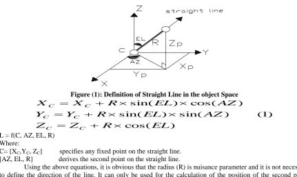
STRAIGHT LINE REPRESENTATION
The straight line feature may be described in several ways. One of them is used to describe the straight linear feature in the three dimensional space mathematically using a fixed point (C) and the curvilinear coordinates of the second point (AZ, EL, R) which both construct the equation of the straight line.
This representation has a physical meaning and can be constructed in the field directly. Referring to any ground coordinates system, point (C) has the coordinates C = [XC, YC, ZC]
Figure (1): Definition of Straight Line in the object Space
) cos(
) 1 ( )
sin( )
sin(
) cos(
) sin(
EL R
Z Z
AZ EL
R Y
Y
AZ EL
R X
X
C C
C C
C C
L = f(C, AZ, EL, R) Where:
C= [XC,YC, ZC] specifies any fixed point on the straight line.
[AZ, EL, R] derives the second point on the straight line.
Using the above equations, it is obvious that the radius (R) is nuisance parameter and it is not necessary to define the direction of the line. It can only be used for the calculation of the position of the second point, which is needed to satisfy the equation of the line. So, the line can be defined only by five parameters, and (R) will be a constant, which has no effect in the adjustment. In this research, (R) is considered as a scalar factor.
2D INTERPOLATION SPLINE REPRESENTATION
A brief discussion of the 2D space Spline feature interpolation will be presented first. Given (m) data set of nodes (control points) [(X1, Y1), (X2, Y2), (X3, Y3) ... (Xm, Ym)] Within the range between the starting point
(a) and the end point (b), there are (m-l) intervals between them. Where each control point is considered as a node in the case of the 2D interpolation spline. These intervals are known as spans. In the cubic polynomial, each span has four coefficients to be determined.
3 3
2 2
1
0
(
)
(
)
(
)
)
(
X
ia
ja
jX
ia
jX
ia
jX
iSY
(2)
Where, 1 < j < m-1 and 1 < i < m.
These give (4m-4) parameters that are needed to describe the spline. From the continuity that inherited in the nature of the spline and also from the first and second derivatives at the (m-2) interior nodes, there are 3 (m-2) equations on the spline (S).
Figure (2): Represents the Spline Curve Interpolation
Next the requirement that the spline (S) passes through the nodes [(X1, Y1), (X2, Y2), (X3, Y3) ...
(Xm, Ym)] as SYj = SY(Xj) gives another (m) equation. Thus, two conditions are needed for the solution of the
Figure (3): Constraints Applied on 2D Spline Curve
Y=(X) = 0 YJ(X) = YJ+1(X) Y¯J(X) = Y¯J+1(X) Y=J(X) = Y=J+1(X)
Y=(X) = 0
DEVELOPMENT OF 3D MATHEMATICAL SPLINE CURVE
Curve (C) in space may be represented with respect to a 3D Cartesian coordinates system being given, we can represent a spline curve by three methods.
A parametric representation of the curve (C), by a vector function r(t) = [x(t), y(t), z(t)]
Parametric representations are useful in many applications, for instance, in mechanics, where (t) represents the time that a body moves along a curve.
Figure (4): Parametric Representations of a Curve in Space
Another type of representation of a curve (C) in space is y = f(x) & z = g(x)
Here, y = f(x) is the projection of (C) into the xy-plane, and Z = g(x) is the projection of (C) into the xz-plane. The third type is the representation of a curve in space as the intersection of two surfaces
F(x, y, z) = 0 and G(x, y, z) = 0
In this section, a new representation of a spline (S) curve feature is presented. A spline S : {S1, S2, S3, ………
Sm-1 } will consist of two- dimensional cubic polynomials SY (Xi) and SZ(Xi) from the three dimensional data
(Xi, Yi, Zi).
From the above, we can see that spline (S) is composed of two individuals one-dimensional polynomial as well as to one-variable, this is shown as:
3 3
2 2
1 0
3 3
2 2
1 0
)
(
)
(
)
(
)
(
)
(
)
(
)
(
)
(
)
(
)
(
i j i
j i j j
i j i
j i j j
i
i i i
j
X
b
X
b
X
b
b
X
a
X
a
X
a
a
X
X
SZ
X
SY
X
S
(3) According to the previous analysis in the 2D interpolation spline, there are no redundancies available in the mathematical model to reduce the effect of the random errors. So, we have to reformulate the mathematical model by considering some of control points as nodes and the others as support points to the interpolation spline. This method is called the form fitting spline. Suppose data sets of (n) control points are available, and (m) control points are selected as nodes. A spline (S) that consists of (m-l) spans will have (m) nodes. This set of nodes consists of (m-2) interior nodes as well as two exterior nodes. The exterior nodes will be called the end points because of their unique positions on the spline (S).
II.
THE
PROPOSED
MATHEMATICAL
MODEL
between a point (XI, YI, ZI) in object space and its corresponding image space coordinates (xi, yi) can be stated
by the linear fractional equations:
1
11 10 9 8 7 6 5
i i i i i i iZ
L
Y
L
X
L
L
Z
L
Y
L
X
L
y
1
11 10 9 4 3 2 1
i i i i i i iZ
L
Y
L
X
L
L
Z
L
Y
L
X
L
x
(4)Where:
L1, L2, L3…L11 are the transformation parameters
Xi, Yi and Zi are the object space coordinates
The mathematical model for calculation the object space coordinates from the direct linear transformation (DLT) coefficients can be stated as follows:
i i I I I i i i i i i y L x L Z Y X L L y L L y L L y L L x L L x L L x 8 4 7 11 6 10 5 9 3 11 2 10 1
9 (5)
Ifwe use the lines as a control points (or in other word by substituting from equation 1 into equation 4), the mathematical model can be stated as follows:
sin(
)
cos(
)
sin(
)
sin(
)
cos(
)
1
)
cos(
)
sin(
)
sin(
)
cos(
)
sin(
11 10 9 4 3 2 1
EL
R
Z
L
AZ
EL
R
Y
L
AZ
EL
R
X
L
L
EL
R
Z
L
AZ
EL
R
Y
L
AZ
EL
R
X
L
x
C C C C C C i
sin(
)
cos(
)
sin(
)
sin(
)
cos(
)
1
)
cos(
)
sin(
)
sin(
)
cos(
)
sin(
11 10 9 9 8 6 5
EL
R
Z
L
AZ
EL
R
Y
L
AZ
EL
R
X
L
L
EL
R
Z
L
AZ
EL
R
Y
L
AZ
EL
R
X
L
y
C C C C C Ci (6)
And if we use the spline curves as a control points (or in other word by substituting from equation 3 into equation 4), the mathematical model can be stated as follows:
( )
( ) ( ) ( )
( ) ( ) ( )
1) ( ) ( ) ( ) ( ) ( ) ( ) ( 3 3 2 2 1 0 11 3 3 2 2 1 0 10 9 4 3 3 2 2 1 0 3 3 3 2 2 1 0 2 1 i j i j i j j i j i j i j j i i j i j i j j i j i j i j j i i X b X b X b b L X a X a X a a L X L L X b X b X b b L X a X a X a a L X L x
( )
( ) ( ) ( )
( ) ( ) ( )
1) ( ) ( ) ( ) ( ) ( ) ( ) ( 3 3 2 2 1 0 11 3 3 2 2 1 0 10 9 9 3 3 2 2 1 0 8 3 3 2 2 1 0 6 5 i j i j i j j i j i j i j j i i j i j i j j i j i j i j j i i X b X b X b b L X a X a X a a L X L L X b X b X b b L X a X a X a a L X L
y (7)
III.
METHODOLOGY
This section describes experiments performed with synthetic images, to evaluate the accuracy obtained from the above mentioned influencing parameters, when the linear features used as control in the 3D space under 1) varying number of linear features (the straight lines & the spline curves as control), 2) different number of fixed points on the straight line, 3) different nodes (control points) on the spline curve. A total of 42 object points, forming a cube with side of 8 meters, will be used as control points, while the rest will be used as check points. To study the geometric characteristics as an essential parameters influencing accuracy, two cases will be taken into consideration, namely double station geometry and three stations geometry. Four different experiments were performed, to assess the influence of the above mentioned parameters. All the double station photographs were performed horizontally in a convergent imaging with 42˚ convergent angle and base distance ratio of one. The first experiment has been performed to study the influence of increasing the number of straight lines upon the accuracy. The solution will be repeated, using different numbers of straight lines, starting with four and ending up with ten increasing one straight line at a time. The second experiment was for studying the effect of increasing the number of points per each straight line; upon the accuracy, 8 pairs were taken for the object array, using four fixed straight lines as control, starting with 3 points and ending up with 10 points per each of the four fixed straight lines, increasing one point at a time. The third experiment was for evaluating the influence of increasing the number of spline curve upon the accuracy, 8 pairs were taken for the object array, starting with 3 spline curves and ending up with ten spline curves increasing one spline curve at a time. The fourth experiment has been performed to evaluate the effect of increasing the interior nodes per each spline curve upon the accuracy. In this experiment, 8 pairs were taken for the object array, using four fixed spline curve, starting with 3 nodes per each spline curve and ending up with 10 nodes per each of the four chosen fixed spline curve increasing one node at a time.
IV.
ASSESSMENT
OF
ACCURACY
whose true coordinates (XT , YT and ZT) are known but not used in the photogrammetric computations. Then, if
the photogrammetric coordinates (XP, YP and ZP) of the check points are computed as new points, an estimation
of the (MRXYZ) spatial residual can be calculated as follows:
5 . 0 2 2
2
1
) ( ) ( ) ( 1
i i i
n
i
Z Y
X n
MRXYZ (8)
Analogous quantities can be estimated for three axes:
The X- direction:
5 . 0 2
1
) ( 1
i
n
i X n MRX
The Y-direction:
5 . 0 2
1
) ( 1
i
n
i
Y n MRY
The Z-direction:
5 . 0 2 1
) ( 1
i
n
i
Z n MRZ
Where:
) (
) (
) (
Ti Pi
Ti Pi
Ti Pi
Z Z Z
Y Y Y
X X X
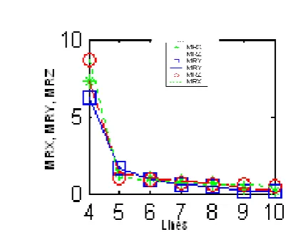
Figure (6): The relationship between number of control lines and evaluated standard deviations (SD) for the object coordinates (in case of using two camera stations)
Figure(5) The relationship between number of control lines and average errors (MRX,MRY,MRZ) for check points (in case of using two camera stations)
Figure (8): The relationship between number of control lines and evaluated standard deviations (SD) for the object coordinates (in case of using
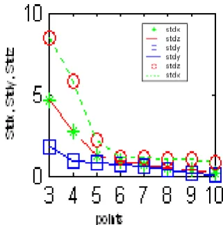
Figure (10): The relationship between number of control points and evaluated standard deviations (SD) for the object coordinates (in case of using two camera stations with 3 lines - multi points per lines)
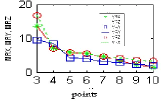
Figure (9): The relationship between number of control points and average errors (MRX,MRY,MRZ) for check points (in case of using two camera stations with 3 lines - multi points per lines)
Figure (12): The relationship between number of control points and evaluated standard deviations (SD) for the object coordinates (in case of using three camera stations with 3 lines - multi points per lines)
Figure (11): The relationship between number of control points and average errors (MRX,MRY,MRZ) for check points (in case of using three camera stations with 3 lines - multi points per lines)
Figure (14): The relationship between number of control points and evaluated standard deviations (SD) for the object coordinates (in case of using two camera stations with 4 lines -multi points per lines)
Figure (16): The relationship between number of control points and evaluated standard deviations (SD) for the object coordinates (in case of using three camera stations with 4 lines -multi points per lines)
Figure (15): The relationship between number of control points and average errors (MRX,MRY,MRZ) for check points (in case of using three camera stations with 4 lines - multi points per lines)
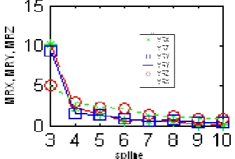
Figure (18): The relationship between number of splines and evaluated standard deviations (SD) for the object coordinates (in case of using two camera stations)
Figure (17): The relationship between number of splines and average errors (MRX,MRY,MRZ) for check points (in case of using two camera stations)
Figure (20): The relationship between number of splines and evaluated standard deviations (SD) for the object coordinates (in case of using two camera stations)
Figure (22): The relationship between number of control points and evaluated standard deviations (SD) for the object coordinates (in case of using two camera stations with 3 splines - multi points per splines)
Figure (21): The relationship between number of control points and average errors (MRX,MRY,MRZ) for check points (in case of using two camera stations with 3 splines - multi points per splines)
Figure (24): The relationship between number of control points and evaluated standard deviations (SD) for the object coordinates (in case of using three camera stations with 3 splines - multi points per splines)
Figure (23): The relationship between number of control points and average errors (MRX,MRY,MRZ) for check points (in case of using three camera stations with 3 splines - multi points per splines)
Figure (26): The relationship between number of control points and evaluated standard deviations (SD) for the object coordinates (in case of using two camera stations with 4 splines - multi points per splines)
Figure (25): The relationship between number of control points and average errors (MRX,MRY,MRZ) for check points (in case of using two camera stations with 4 splines - multi points per splines)
Figure (28): The relationship between number of control points and evaluated standard deviations (SD) for the object coordinates (in case of using three camera stations with 4 splines - multi points per splines)
V.
ANALYSIS
AND
DISCUSSION
OF
THE
RESULTS
This section will include the results performed for the accuracy assessment of different experiments parameters according to the assessment criteria.
i) Effect of different numbers of straight line:
In this experiment, the influence of increasing the straight lines upon the accuracy will be studied. The improvements in the statistics of discrepancies will be illustrated in figure (5) and (7), while the improvements in the statistics of positional standard deviations will be showed in figure (6) and (8), the obtained results show the following:
- There is a significant improvement in all assessment criteria, when the number of straight lines increased from 4 to 5.
- There is a slight improvement in accuracy, when the straight lines are between 5 and 9.
- There is no significant improvement in accuracy, when the numbers of straight lines increased than 9.
ii) The effect of increasing the laying points on the straight lines upon the accuracy
In this experiment, the influence of increasing the number of points on the straight lines upon the accuracy will be evaluated. From figure (9) to figure (16), one can notice that:
- There is a significant improvement in all assessment criteria, when the number of points increased from 3 to 5. -There is a slight improvement in accuracy, when the number of points increased from 5 to 9.
-There is no significant improvement when the numbers of points increased than 9 points.
iii) Effect of different numbers of spline curves
The effect of increasing the numbers of spline curves in improving the results will be handled. The obtained results are presented in a figural form. Figure (17), (19) illustrates the improvements in the statistics of discrepancies, while figure (18), (20) gives the improvements in the statistics of positional standard deviations. The obtained results from the different experiments will be analyzed here and discussed. This will be achieved through the careful examination of figure (17) to figure (20)
From figures (17) to figure (20), one can notice that:
-There is a significant improvement in all assessment criteria, when the numbers of spline curves increased from 3 to 4.
-There is a slight improvement in all assessment criteria, when the numbers of spline curve increased than 7.
iv) Effect of increasing nodes that described the spline curved (effect of increasing interior nodes):
In this experiment, the effect of increasing the number of interior nodes in improving the results will be studied. It is to be said, that we used 4 spline curves. spline curve each time also be increased simultaneously for each of the used 4 spline curve. The interior nodes are starting with 3 nodes and ending up with ten, increasing one node at a time. It is to be noted that, the interior nodes have been equal distributed on all used spline curve. Figures (21), (23), (25) and (27) illustrates the improvements in the statistics of discrepancies, while figure (22), (24), (26) and (28) gives the improvements in the statistics of positional standard deviations. From figure (21) to figure (28) one can notice the following:
-There is a slight improvement in all assessment criteria, when the number of nodes increased from 3 to 4. -There is a significant improvement in all assessment criteria, when the number of nodes increased from 4 to 5. -The improvement in accuracy will be continued until the number of nodes reaches to 9.
-There is no significant improvement in accuracy, when the number of nodes increasing than 9.
VI.
CONCLUSIONS
REFERENCES
[1]. Dalati, "Potentials of Using Linear Features in the Photogrammetric Reduction Processes and Its Applications in Cadastral Surveying", PhD. Thesis, Faculty of Engineering, Cairo University, Egypt 1989 .
[2]. Habib, A., Morgan M. F. "Linear Features in Photogrammetry", Technical Report, Department of Geomatics Engineering, University of Calgary, CANADA, 2008.
[3]. Hottier," Accuracy of close -Range Analytical Restitutions: Practical Experiments and Prediction" Photogrammetric Engineering and Remote sensing,Vol.42, pp. 345-375 March, No.3, 1976
[4]. Morgan M. F.,"Linear Features in Photogrammetry", Technical Report, Department of Geomatics Engineering, University of Calgary, CANADA, 2008
[5]. Mulawa, D. C., "Estimation and photogrammetric Treatment of Linear Features " Ph.D. Thesis, purdue University, USA ,1989.
[6]. Mulawa, D., and Mikhail, E., "Photogrammetric reduction of automatically extracted linear features of three dimensional models", Interim Technical Report, Purdue University, no. CE-PH-88-9,. 1988 [7]. Torlegard, K., “Accuracy improvement in close range photogrammetry" Heft 5, Munchen, September,