On the use of sensitivity tests in seismic tomography

(1)

Geophysical Journal International

Geophys. J. Int.(2016)205,1221–1243 doi: 10.1093/gji/ggw084

Advance Access publication 2016 March 7 GJI Seismology

On the use of sensitivity tests in seismic tomography

N. Rawlinson

1

and W. Spakman

2,3

1_{School of Geosciences, University of Aberdeen, Aberdeen, Scotland AB}_{24 3}_{UE. E-mail:}_{[email protected]}

2_{Department of Earth Sciences, Faculty of Geosciences, Utrecht University, PO BOX}_{80115, 3584}_{TC, Utrecht, The Netherlands} 3_{Centre of Earth Evolution and Dynamics (CEED), University of Oslo,}₀₃₁₆_{Oslo, Norway}

Accepted 2016 February 29. Received 2016 February 15; in original form 2015 October 15

S U M M A R Y

Sensitivity analysis with synthetic models is widely used in seismic tomography as a means for assessing the spatial resolution of solutions produced by, in most cases, linear or iterative nonlinear inversion schemes. The most common type of synthetic reconstruction test is the so-called checkerboard resolution test in which the synthetic model comprises an alternating pattern of higher and lower wave speed (or some other seismic property such as attenuation) in 2-D or 3-D. Although originally introduced for application to large inverse problems for which formal resolution and covariance could not be computed, these tests have achieved popularity, even when resolution and covariance can be computed, by virtue of being simple to implement and providing rapid and intuitive insight into the reliability of the recovered model. However, checkerboard tests have a number of potential drawbacks, including (1) only providing indirect evidence of quantitative measures of reliability such as resolution and uncertainty, (2) giving a potentially misleading impression of the range of scale-lengths that can be resolved, and (3) not giving a true picture of the structural distortion or smearing that can be caused by the data coverage. The widespread use of synthetic reconstruction tests in seismic tomography is likely to continue for some time yet, so it is important to implement best practice where possible. The goal of this paper is to develop the underlying theory and carry out a series of numerical experiments in order to establish best practice and identify some common pitfalls. Based on our findings, we recommend (1) the use of a discrete spike test involving a sparse distribution of spikes, rather than the use of the conventional tightly spaced checkerboard; (2) using data coverage (e.g. ray-path geometry) inherited from the model constrained by the observations (i.e. the same forward operator or matrix), rather than the data coverage obtained by solving the forward problem through the synthetic model; (3) carrying out multiple tests using structures of different scale length; (4) taking special care with regard to what can be inferred when using synthetic structures that closely mimic what has been recovered in the observation-based model; (5) investigating the range of structural wavelengths that can be recovered using realistic levels of imposed data noise; and (6) where feasible, assessing the influence of model parametrization error, which arises from making a choice as to how structure is to be represented.

Key words: Inverse theory; Seismic tomography.

1 I N T R O D U C T I O N

The effective assessment of model reliability is still a major chal-lenge in seismic tomography despite over four decades of devel-opment. The ill-posed nature of the tomographic inverse prob-lem means that multiple data-satisfying solutions exist, and these solutions tend to be unstable with respect to small changes in data noise and initial conditions unless regularization is applied (Rawlinsonet al.2014). The combination of implicit (e.g. via choice of a model parametrization) and explicit (e.g. damping and

smooth-ing) regularization, a poor knowledge of data noise, uncertainty in prior information, and simplifying assumptions made in the for-ward and inverse step (e.g. using the ray approximation, ignoring anisotropy, linearization) actually make it extremely difficult for any method to provide a reliable assessment of model robustness.

The pioneers of geophysical inverse problems (Backus & Gilbert 1967,1968,1970; Franklin1970; Wiggins1972) and seismic to-mography (Aki & Lee1976; Akiet al. 1977) clearly recognized the importance of assessing solution robustness and the need to try and quantify uncertainty. For example, in both the local earthquake

C

The Authors 2016. Published by Oxford University Press on behalf of The Royal Astronomical Society. 1221

at University of Aberdeen on April 26, 2016

http://gji.oxfordjournals.org/

(2)

tomography study of Aki & Lee (1976) and the teleseismic tomog-raphy study of Akiet al.(1977), formal estimates of posterior co-variance and resolution are made for all model unknowns. Despite the massive increases in computing power and ongoing theoreti-cal developments that have taken place since these seminal works, progress in the assessment of model robustness has been limited. As well as estimates of posterior covariance and uncertainty from linear theory, other methods that have been tried include synthetic reconstruction tests, jackknife and bootstrap methods and sampling strategies (for a review see Rawlinsonet al.2014).

For small to medium-sized linear or linearizable inverse prob-lems, the calculation of posterior covariance and resolution is rel-atively straightforward, and has been frequently used as a measure of solution reliability in seismic tomography (e.g. Akiet al.1977; White1989; Zelt & Smith1992; Stecket al.1998). For larger

prob-lems, approximation methods have been applied (e.g. Yao et al.

1999; Zhang & Thurber2007), although care must be taken when iterative solution methods like LSQR, which only explore a re-stricted subspace of the full model space when the number of itera-tion steps is limited, are used (Noletet al.1999). However, while the attainment of quantitative estimates of model uncertainty and spa-tial resolution is attractive, the general limitations associated with the tomographic inverse problem, as described earlier, means that at the very least the absolute value of these quantities are poorly constrained. Moreover, their validity decreases as the nonlinearity of the inverse problem increases.

An alternative to directly computing resolution or posterior co-variance is to instead target a proxy such as resolution length. For example, Fichtner & Trampert (2011) develop a method for full waveform inversion problems, based on low-rank approximations of the Hessian operator that can determine the 3-D distribution of direction-dependent resolution lengths with potentially greater computational efficiency than a synthetic test. This approach can be viewed as a generalization of the ray density tensor (Kissling1988), which quantifies space-dependent azimuthal coverage. More re-cently, Fichtner & van Leeuwen (2015) develop and apply a random probing technique for resolution analysis that avoids the algorith-mic complexity and computational requirements of the Fichtner & Trampert (2011) method. In addition, it can be applied to any tomo-graphic technique, including full waveform inversion and linearized ray tomography. A thorough comparison between this technique and more traditional methods of resolution analysis is yet to be carried out.

Sensitivity analyses, or synthetic reconstruction tests, are the most common method for assessing solution robustness in seismic tomography, and were originally introduced to investigate spatial resolution in inverse problems for which formal resolution can-not be computed due to the large model size (Spakman & Nolet 1988). They involve the formulation of a heterogeneous synthetic model through which the forward problem is solved using the iden-tical data coverage as the observational data set. The inversion method is then applied to the synthetic data set in an effort to re-cover the test model. Differences between the true and rere-covered model provide a basis for assessing the reliability of the solution. Input structures range from single discrete spikes (Walck & Clay-ton1987; Rasmussen & Humphreys1988), to widely spaced spikes (Grand1987; Spakman & Nolet1988), to tightly spaced checker-boards (Inoueet al.1990; Fukaoet al.1992; Glahn & Granet1993; Zhaoet al.1996; Zelt & Barton1998; Gorbatovet al.2000; Fish-wicket al.2005; Chen & Jordan2007; Yanget al.2009; Rawlinson

et al.2011) to structures designed to investigate particular features such as subduction zones (Spakmanet al.1989; Eberhart-Phillips &

Reyners1997; Bijwaardet al.1998; Graeber & Asch1999; Wolfe

et al.2002). Of these, the tightly spaced checkerboard pattern of alternating positive and negative anomalies (relative to some ref-erence structure) is by far the most common, but also the most criticized. For example, L´evˆequeet al.(1993) clearly show that it is possible to devise data geometries for which small-scale structures (as is commonly used in a checkerboard test) are well retrieved while larger scale structures are poorly retrieved. More generally, their re-sults show - unsurprisingly - that the recovery has a dependence on the choice of the synthetic model.

Standard statistical methods of error assessment such as jack-knife and bootstrap tests have seen limited use in seismic tomog-raphy (Lees & Crosson1989,1990; Su & Dziewonski1997; Zelt 1999; Gung & Romanowicz2004). Both methods rely on running repeat inversions with various subsets of the data set (via resam-pling in the case of bootstrap, and omission in the case of jackknife) and interrogating the ensemble of solutions that are produced for summary information. One of the main limitations of both meth-ods is that they require an overdetermined inverse problem in or-der to work effectively (Noletet al.1999), which rarely occurs in practice.

The idea of sampling regions of model space in which the data are satisfied in order to produce an ensemble of solutions is gradu-ally becoming more common, thanks in part to ongoing increases in computing power. Within a linear or weakly nonlinear framework, a number of different techniques have been tried, including multiple starting models (Vascoet al.1996), the so-called ‘null space shut-tle’ (Deal & Nolet1996; de Witet al.2012), regularized extremal

bounds analysis (Meju 2009), Lie group methods (Vasco 2007)

and the dynamic objective function scheme (Rawlinson & Kennett 2008). However, it is in the realm of fully nonlinear sampling where the greatest strides are currently being made. For example, Bayesian trans-dimensional tomography, in which the number of unknowns is an unknown itself, and the parametrization is adaptive, is starting to become increasingly popular. It has been shown to be computa-tionally tractable for most 2-D and some 3-D problems (Bodin & Sambridge2009; Bodinet al.2012; Younget al.2013; Galettiet al.

2015; Piana Agostinettiet al.2015; Hawkins & Sambridge2015), and generates a large ensemble of solutions which can be used to quantitatively assess solution reliability. In general, these methods have an intrinsic parsimony which results in a (variable) spatial res-olution that contains only structure that is ‘required’ by the data; the uncertainty associated with structure at this spatial resolution can be estimated by taking the standard deviation of the solution ensemble.

In this paper, we focus on establishing best practice for the im-plementation of sensitivity analysis, which has become the standard approach for assessing solution quality in seismic tomography, even when the resolution matrix can actually be computed (in which case, the recovery of any test structure can be rapidly obtained; see Section 2). As well as results and findings from previous studies, these guidelines are founded in theory and informed by a series of numerical tests that use both synthetic data (see Section 3) and data recorded in the field (see Supporting Information). Note that we only consider tomographic inverse problems that are linear or weakly nonlinear. As such, it is assumed that the starting model is sufficiently close to the required minimum of the objective function that the assumption of local linearization will allow the solution to enter a region of acceptable data-fit (whether by a single step or iteratively) within the neighbourhood of this minimum. If this is not the case, then the problem may require a fully nonlinear solver and consequently a different approach to assessing solution robustness.

(3)

2 T H E O R E T I C A L C O N S I D E R AT I O N S

Our aim in this section is to provide a theoretical framework for the proper use of spatial resolution and noise analysis with synthetic models in tomographic inverse problems that solve a linear(ized) system of equations. In addition, we address how implicit formula-tions of the inverse problem that focus on minimizing a cost function may adhere to this theory.

2.1 The forward problem

The general nonlinear forward problem of noise-free datadE (e.g.

traveltimes, waveforms, some portion of the seismogram) can be written asdE =g(mE)+t, wheremErepresents the distribution

of some true-Earth seismic property (e.g.P-wave velocity) andgis a nonlinear integral operator. The errort represents the discrepancy

betweendEand its theoretical predictiong(mE) and the magnitude

oft is a function of the approximations made in solving the

for-ward problem. For example, the tomographic inverse problem in its simplest form, using ray theory, is nonlinear and the finite fre-quency traveltimedE may be inconsistent with the theoretical ray

predictiong(mE).

If we now add observational noised (e.g. picking error), such

thatd=dE+d, then

d=g(mE)+t+d. (1)

Next, assuming a suitable model parametrization that projectsmE

on the model vectormp, this leads to

d=g(mp)+t+d+p. (2)

wherep is the implied parametrization error. In the explicit

for-mulation that we follow here, the next step is defining the matrix representation of the integral equations as a locally linear represen-tation ofg(mp) about the true modelmp, so that

dp=Gpmp (3)

wheredp =g(mp) andGp is the observation matrix relating the

datadpto the true Earth modelm. We assume that this relationship

is exact, so that substitution into eq. (2) yields

d=Gpmp+t+d+p. (4)

Note that from the inversion viewpoint, eq. (4) is still a nonlinear relationship between observationsdandmp becauseGp andmp

are both unknown and in additionGpgenerally depends onmp. For

instance, in ray-based tomography,Gpis obtained from integration

along the 3-D geometry of the true ray paths that depends on the true modelmp.

For a linear(ized) inversion of eq. (4) one assumes an approxima-tionG=GpwhereGis a known matrix obtained from integration

over a background reference model. This leads to an additional inconsistency between the data and model predictions, which we denote with the linearization errorl. For later use we formalize

this as follows

Gpmp=(G−E)mp=Gmp+l (5)

whereE=(G−Gp) is the linearization error in the observation

matrix.

The forward equation of a linearized inversion thus becomes

d=Gmp+, where=d+l+t+p. Although the

obser-vational errorsdcan be random, the implicit data errors may have

a systematic component, which would likely manifest more promi-nently in the tomographic solution. In tomographic formulations

of the inverse problem, data errorsare often represented by the data covariance matrixCd, which in theory can accommodate all

variances and error correlations.

Due to a lack of data and the presence of data errors, the tomo-graphic inverse problem is generally underdetermined or

mixed-determined (Tarantola1987; Menke 1989). Consequently, a null

space exists in which modifications can be made to mp without

changing the datad. As a result, we cannot expect to retrievemp

from the inversion ofd=Gmp+, as it is only one of many

data satisfying solutions. To make this explicit,mp is replaced by

m, which denotes any model that can fit the data equally as well asmp based on an adopted measure of data fit. This leads to the

well-known form of the linearized forward equation

d=Gm+ (6)

where we make explicit that=d+t+l+p comprises all

sources of observation error and errors introduced by the various assumptions that we have outlined above.

2.2 The linearized inverse problem and the resolution matrix

Here we take a generalized and practical approach to tomographic inversion which is largely independent of the number of model pa-rameters and volume of data. The two main features are (1) solution of a linear/linearized inverse problem, and (2) assessment of solu-tion robustness either via computasolu-tion of the resolusolu-tion matrix or sensitivity analysis. In general, sensitivity analysis is the only way to assess solution characteristics for problems involving a very large number of inversion parameters.

Formulation of the tomographic inverse problem starts with the design of a data misfit function, which is usually extended by the addition of one or more regularization terms which penalizes model attributes, such as model amplitude, flatness and/or smoothness (Menke1989). Notions about prior model covariance are also used to precondition the inverse problem (e.g. Rawlinsonet al.2014). The penalty term serves to deal with the underdetermined nature of the inverse problem, usually by trying to exclude models which exhibit levels of detail not required by the data. A basic example is the cost function associated with the linearized and regularized least squares inversion (Rawlinsonet al.2010):

S(m)=(d−Gm)T_C−1

d (d−Gm)+α

2_mT_DT_Dm ₍₇₎

The first term is the quadratic data misfit scaled by the prior data covarianceCd and the second term defines the penalties on model

attributes through a pre-designed damping matrixαD. The tuning parameterα regulates the trade-off between fitting the data and satisfying the model penalties.

In order to solve the inverse problem, the next step is to find the model ˆmwhich minimizes the adopted cost functionS(m). For linear problems, the solution can be formally written as

ˆ

m=G−gd (8)

whereG−g _{is the so-called generalized inverse (Backus & Gilbert}

1970). For eq. (7), the generalized inverse has the form (e.g. Rawlinsonet al.2014)

G−g₌_GT_C−1 d G+α

2_DT_D−1_GT_C−1

d (9)

This illustrates that generallyG−g_{is not unique and is dependent on}

Cd, representing all data errorsd, and on the adopted regularization

operatorαD.

(4)

If we now substitute the relationship between the observations and the true Earth model of eq. (4) into eq. (8), we obtain an instructive equation that shows how the true Earth model and actual data errors map into the tomographic solution

ˆ

m=Rpmp+G−g(d+t+p) (10)

where

Rp=G−gGp (11)

is the true spatial resolution matrix and defines the linear depen-dence of each model parameter ˆmion components of the true model

mp. In effect, it measures the amount of ‘blurring’ produced by the

inverse operator. IfR=I, then there is no blurring and the least squares solution has perfect resolution.

For a linear inverse problemGp =G, and hence the resolution

matrix can formally be computed. Instead, for a linearized problem, which is the usual case in seismic tomography, we do not know

Gp. However, by inserting eq. (5) into eq. (10), we can arrive at a

useful equation which allows for a practical implementation of eqs (10) and (11) and explicitly shows the role of the linearization error, which is not present in eq. (10):

ˆ

m=Rmp−G−gEmp+G−g(d+t+p) (12)

or ˆ

m=Rmp+G−g (13)

whereR=G−g_G_{is the more commonly used resolution matrix}

(e.g. Nolet2008). Eq. (12) demonstrates thatRcan only be consid-ered to be an approximation to the true resolution matrixRpin case

of a linearized inverse problem, that is,Rp=R−G−gE. This is

an important observation that has an analogy when considering the spatial resolution of the final model of a nonlinear inversion (see below).

The error termG−g_{in eq. (13) includes the linearization error}

and explicitly accounts for the propagation of all data noise into the solution. As this noise is unknown, it cannot be computed except in controlled synthetic experiments. As an approximation, the effect of data errorson the solution is estimated from the propagation of the prescribed data covarianceCd into the posterior model

covari-anceCM. Since the covariance of any linear combinationApof a

Gaussian distributed random variablepis Cov(Ap)=ACov(p)AT_,

then the posterior covariance of the model parameters is (using eq. (8))

CM =G−gCd(G−g)T (14)

Thus, the model covariance for a least squares inverse problem depends on the data errors and not the data itself (sinceG−g_{is not}

a function ofd), so any assumptions used in the construction ofCd

will also determine the quality of the tomographic solution.

2.3 Sensitivity analysis with synthetic velocity models

For tomographic inverse problems of the class described above (linear/linearized least squares), it has long been recognized that

the computation ofRmay not be practical when large numbers of

model parameters are involved. Motivated by the form of eq. (13), this has led to the use of sensitivity analysis with synthetic models and synthetic data (e.g. Spakman & Nolet1988). This is carried out by constructing a synthetic modelms (e.g. a checkerboard or

spike model), from which synthetic data are computed by forward solution withG, and by optionally adding synthetic noise yielding

ds=Gms+s. (15)

Solving ds =Gm+s in the same way as eq. (6) leads to the

solution model ˆms, and analogous to eq. (13), ˆms relates to the

synthetic modelms as

ˆ

ms=Rms+G−gs (16)

Because the resolution matrixRin eqs (16) and (13) are identi-cal, sensitivity analysis with noise-free synthetic data constitutes a correct basis for inferring properties ofRfrom the comparison of the synthetic modelms with the tomographic solution ˆms.

Exper-iments that are restricted to inverting synthetic noise, in effect by takingms =0 and inverting a synthetic noise vector, can be useful

to assess the importance of the second term in eq. (13). Inversion of noisy synthetic data is used to examine the combined effects of lack of resolution and noise propagation on the tomographic solution (see Rawlinsonet al.2014, for more details). However, it is worth noting that the full information content ofRcannot be retrieved from a single synthetic test, even in the absence of imposed data noise, because Ris not uniquely constrained by the relationship

ˆ

ms=Rms. If the full blurring effects are to be understood, then a

spike test for each model parameter would need to be run indepen-dently, and the results collated. A single spike test of this sort would retrieve the information equivalent of only one column or row ofR.

2.4 Nonlinear inversion and sensitivity analysis

In nonlinear inversion, a set of observations d of the nonlinear integral functional g(mp) is used for developing a model space

search for the modelmp. As before, we writed=dp+such that

the exact equation isdp=g(mp). Note that=d+t+p and

does not include the linearization errorl. By defining a weighted

cost function||d−g(m)||wa sequence of modelsmk_,_k₌_{1, . . . ,}_K

can be created (usually under the assumption of weak nonlinearity), that aims at sequentially minimizing ||d−g(m)||w such that at

convergence we have found a model ˆm≈mK _{with an acceptable}

data misfit||d−g( ˆm)||w≈ ||||w. An example of the objective or cost function is

S(m)=(d−g(m))TC−d1(d−g(m))+α 2

P(m) (17) whereP(m) stands for any combination of regularization and prior model information.

Ifdk _{is the prediction of}_d_{after step}_k_{, the nonlinear equation}

dk₌_g₍_mk_{) is formally represented by} _dk₌_Gk_mk _where _Gk _is

the observation matrix associated withmk_{. Similarly, we can write}

d=Gmˆ +ˆ for the final solution ˆm=mK _and_d

p =Gpmp for

the true solution. The different data errors (and ˆ) reflect the risk of irrecoverably mapping part of the original errors into the solution while stepping through model space. A nonlinear inversion scheme particularly aims to improve the solution of the forward problem

such thatGk_→_G

pand consequentlymk→mp. For weakly

non-linear problems,Gk _{is created explicitly as a result of step-wise}

linearization. Strongly nonlinear tomographic problems are often solved via a direct model-space search and do not necessarily in-volve an explicit formulation ofGk_{. This class of solution strategy}

can also address pure least squares formulations of the inverse prob-lem (α=0 in eq. 17), but in this case ad hoc decisions are usually required to choose what can be regarded as acceptable models, for example, selecting the minimum norm solution.

(5)

In a linearized inverse problem, we implicitly accept thatG≈ Gp, orG=Gp+E(see eq. 5). In nonlinear inversion we want

to improve on this approximation, but the attempted convergence

Gk_→_G

p generally gives rise to the problem of nonlinear error

propagation. For example, in ray-based tomography a step-wise linearization of the inverse problem requires 3-D ray tracing at step

kthrough modelmk_{, which is required for determination of the next}

observation matrix Gk+1_{. Model errors in}_mk _{(i.e. lack of spatial}

resolution and model amplitude error) cause errors in the 3-D ray geometries that propagate intoGk+1_{, which is subsequently used to}

invert formk+1_{. Lack of spatial resolution at each step may prevent}

ray geometry errors from being corrected in subsequent steps and can even accumulate during iteration. This affects the convergence to the final model in an intractable way and may force convergence to a local minimum of the misfit function||d−g(mk₎_||w_{. Hence, as}

a result of data errors, of insufficient data constraints and possibly

of the model search strategy used, the model mk+1 _{depends on}

previous models and contains model errors as a result of nonlinear errors that propagated intoGk+1_{, which was used for determining} mk+1_{. This generally affects the convergence}_Gk_→_G

psuch thatG

does not necessarily converge toGp and consequentlymkdoes not

necessarily converge tomp. In analogy with the linearized inversion

(Section 2.2), we express this error asE=G−Gpfor the accepted

final model ˆm=mk_.

The above general description allows for the creation of a the-oretical starting point for the application of sensitivity analysis to the solution of nonlinear inverse problems. For the final solution ˆm

we can formally write ˆm=G−g_d_{(see eq. 8). Here, the generalized}

inverseG−g_{stands for a repeatable inversion process to obtain the}

solution ˆm, or for an explicit operator obtained from the last inver-sion step, and incorporates the propagated forward problem error

E. Thus we can write ˆ

m=G−g(dp+)=G−g(Gpmp+)=G−g((G−E)mp+)

=Rmp−G−g(Emp−). (18)

This equation is analogous to eq. (13) that was obtained for a one-step linearization inversion where we also hadR=G−g_G_{. A similar}

equation holds at each step kof the nonlinear inversion scheme.

The term G−g_Em

p accounts for the data error that results from

convergence of the nonlinear solution scheme to ˆminstead ofmp,

which is due to the nonlinear propagation of data and model errors and includes linearization errors. Note that in eq. (13) the original data error occurs and that by implication the errorEinGabsorbs all the nonlinear error propagation. As for linearized inversion, the true resolution matrix isRp =G−gGp=G−g(G−E), but in this case

R=G−g_G _{cannot exactly describe the spatial resolution matrix}

for the final result of a nonlinear inversion due to nonlinear error propagation. In practice, however,Rwill be our best guess of the resolution matrix because we can computeGbut notGp. Therefore,

synthetic datadsfor sensitivity analysis of the solution ˆmcan only

be generated byGms =ds.

The use of eq. (18) for sensitivity analysis aimed at retrieving aspects ofRpis therefore approximate, as was the case for a one-step

linearized inverse problem where the difference matrixEaccounted for only the linearization error (see Section 2.2). On a practical note: similar to a one-step linearized inverse problem, the matrixGwith which the final solution ˆmis computed could still be improved by using ˆmif convergence has not been achieved. For instance, in

ray-based tomography, one could perform ray tracing through ˆmand

construct an improved observation matrixG. The improvedGcan

then be used in eq. (18) which would further reduce the linearization errorEand may improve the approximation ofRtoRp.

In summary, sensitivity analysis applied to the last stage of an iterative nonlinear inversion scheme for solution ˆm leads to the inferenceR=G−g_G_{, which is an approximation of the true}

reso-lution matrixRp =G−g(G−E). The size of the propagated

non-linear resolution errorG−g₍_E_{) will determine the accuracy of the}

approximationR≈Rp.

In sensitivity tests we effectively assumeE=0, which implies the same strengths and limitations of sensitivity analysis as in a purely linear inversion, albeit with the additional uncertainty of the second error propagation term−G−g_Em

p. Eq. (18) does,

how-ever, provide a general means to investigate effects of nonlinear error propagation by explicitly computing this term in a designed synthetic experiment that starts with creatingds andGsfor a

syn-thetic modelms such thatds=Gsms. Next, a nonlinear inversion

can be started from some modelm1

s that converges to the equation

ˆ

ds =Gmˆs. This allows for the evaluation ofE=G−Gs. Similarly,

given a particular source and receiver network, one can use eq. (18) as a basis for investigating if certain perceived Earth structure (e.g. slab geometry; gap in slab) can be resolved by the nonlinear inver-sion scheme in use. Note that all such experiments fundamentally depart from testing the spatial resolution (i.e. the algebraic relation-ship between model parameters) of the real data experiment, that is, belonging to ˆm, as bothG−g _and_G_{will generally be different}

in synthetic experiments that solve the forward problem forms, for

example, by 3-D ray tracing throughms.

We note that ifG−g_{can be reproduced independent of}_m sthen

the designed amplitudes ofmsdo not influence sensitivity analysis

because we are performing a strictly linear inversion for ˆms aimed

at estimating algebraic properties ofR. However, if this is not the case and the entire nonlinear scheme needs to be repeated, then an approximate alternative is to superimposemsas a synthetic pattern

on the data-generated solution ˆm, such that the synthetic data are computed as G1_{( ˆ}_m₊_m

s) as the starting data set for nonlinear

inversion (Zelt1998). This may mimic a comparable convergence

sequenceGk_→_G_{if the amplitude of}_m

s are a sufficiently small

fraction of ˆms such that they do not lead to additional nonlinearity

and error propagation.

2.5 Theoretical implications for sensitivity analysis

For proper application and interpretation of sensitivity analysis, the following implications that arise from the theory outlined in Sections 2.1–2.4 are now discussed.

(i) Sensitivity analysis only applies to linear systems like eqs (6) and (15) and implicitly assesses the linear dependence between

model parameters as defined byR and explicitly assesses noise

propagation into the solution viaG−g

s. However, it does not assess

the effects of all assumptions and approximations that were made to convert the nonlinear inverse problemd=g(mE)+t+dinto

the linearized inverse problemd=Gm+d+t+l+p. This

is not a specific weakness of sensitivity analysis, because it also applies whenRis explicitly computed. However, one advantage of sensitivity analysis is that it does allow the influence of the error term in eq. (13) to be analysed (see Sections 3.4, 3.5, 3.7 and 3.9 for examples).

(ii) It follows fromR=G−g_G_{that if the synthetic model} _m s

lies in the null space of G, then Rms=0=mˆs and there will

be no recovery in a synthetic experiment. Conversely, any model

ms that is entirely in the row space of G (i.e. maps only in the

(6)

range ofG) can be fully recovered (ms=mˆs). Sensitivity analysis

may lead to an incomplete interpretation ofR when applied to

the two end-member models. L´evˆequeet al.(1993) demonstrated this in an idealized experiment that showed perfect recovery for a spatially detailed checkerboard model, while a coarse checkerboard was almost entirely in the null space ofG, despite identical path coverage. By implication,sensitivity tests can only be used to expose a lack of resolution. Resolution artefacts should be inferred from sensitivity tests using a wide variety of synthetic models in an attempt to explore all null space components (e.g. Bijwaardet al.

1998). Spatial scale dependence of sensitivity tests is illustrated with experiments in Section 3.5.

(iii) A synthetic model that consists of only one value for model parameteri(a spike) and zeros elsewhere leads to the determination of theith row and column of the resolution matrix (Spakman & Nolet 1988). Spakman & Nolet (1988) specifically devised the ‘spike model’ comprising a regular grid of well-separated spikes with zeros in between as a more economic way of obtaining a mapping of many columns ofRin one inversion. Still, the interpretation pitfall exposed by L´evˆequeet al.(1993) may theoretically occur such that a particular choice of synthetic model may not sufficiently detect lack of resolution. Therefore, as noted before, sensitivity analysis should be conducted with a variety of different synthetic models covering all scale-lengths to optimize thedetection of lack of resolution(see Section 3.5).

(iv) Note that eq. (16) requires that sensitivity tests should use in eq. (15) the matrixGof eq. (6) for computation of synthetic data and, in addition, theG−g_{used in ˆ}_m₌_G−g_d_{for inversion. If}_G−g

is not explicitly available then the synthetic inversion must mimic the real data inversion to the extent that the use of the sameG−g_is

implied (this would apply equally to finite frequency tomography for example, where one should use the finite frequency kernels built for the real data paths in any sensitivity test involving a synthetic model). If we instead construct a matrixGin eq. (15) from 3-D ray tracing (for example) through the synthetic modelms, then this leads

to a differentGthan in eq. (6), so the resolution matrixR=G−g_G

in eq. (16) is not the same as in eq. (10). This is illustrated in

Section 3.3. Also, the synthetic model ms should be defined on

the same model parametrization as used for the construction of

Gotherwise model projection noisep (see eq. 6) will enter the

analysis though the second term in eq. (10). This is illustrated in Section 3.9.

(v) Eq. (16) implies that noise-free synthetic data should be used if the sensitivity analysis focuses only on assessing the properties of

R. As mentioned in the previous section, inversion of only synthetic noise assesses the importance of the second term in eq. (6), while the inversion of noisy synthetic data explores the combination of the two terms. Synthetic noise can be generated that has a distribution consistent with that assumed for the real data by means of the data covariance (e.g. Gaussian). The signal-to-noise ratio can be tuned such that the same data misfit is obtained as in the real-data inversion (Spakman & Nolet1988). This, however, is still approximate, as we do not know the real data errors. Section 3.8 explores the effect of data noise in the recovery of structure.

(vi) The second term in eq. (16),G−g

s, opens the possibility to

investigate how a wide variety of random or systematic data noise can propagate into the solution. For instance, tests can be devised for the influence on a tomographic model of the projection error due to model parametrization (as is done in Section 3.9). Propagation of random noise can be studied to detect noise-sensitive regions of the model. A special case is the ‘permuted data test’ (Spakman &

Nolet1988; Spakman1991), in which the data vector in eq. (6)

is randomly permuted prior to inversion. The application of this technique to global traveltime tomography led to a data-derived estimate of average model amplitude error (Bijwaardet al.1998).

(vii) The linear nature of eq. (16) implies that the inversion re-sponse to any synthetic model can be obtained from a superposition of single-spike responses (ignoring the effect ofs), that is,

ˆ ms=Rms =R n anmspiken = n anmˆspiken (19)

whereai,i=1, . . . ,nis a scaling coefficient. In particular,

checker-board models can be seen as a superposition of synthetic models with a regular distribution of spikes. This suggests that inferring res-olution artefacts from checkerboard models can be more complex than for each of the separate spike models. This will be investigated in Sections 3.1 and 3.2.

(viii) Care should be taken when conducting sensitivity exper-iments with the observational model, that is, the model obtained from inverting the real data. When using it as a synthetic model, one can expect an almost identical output. The part of the model that is built from the row space ofG(i.e. data constrained), will be completely recovered. Merged with this is a null space compo-nent that is shaped and constrained by the applied regularization. This leads to linear dependencies between model parameters that are fully described byRand which, hence, describes their mapping in the observational model. From a theoretical point of view the observational model is defined by ˆm=Rmp; if we take ˆmas our

synthetic model, then ˆms =RRmp. IfRis an idempotent matrix

(RR=R), then ˆms=mˆ and the input and output models should

be identical. While this may not be true in general, our tests seem to indicate that for our chosen objective function, the corresponding resolution matrix is likely to be at least quasi-idempotent (RR≈R), as demonstrated in Section 3.6.

What can be done successfully is to construct synthetic models by removing a certain feature from the observational model, for example, a slab in a mantle model, and test if it fully reappears in

ˆ

ms, in which case it is a resolution artifact. In the end-member case

of setting the amplitude of only one model parameter to zero in the observational model, that is, applying an ‘anti-spike’, a correct estimate is obtained in the recovered model of how the ambient model contributes to amplitude and sign imaged for this parameter. This exposes the summed contribution of all off-diagonal elements in the pertinent row ofRin determining the value (see Supplemen-tary Information for an example). These are very powerful ways of testing specific attributes of the observational model.

3 N U M E R I C A L E X P E R I M E N T S

In order to conduct our numerical experiments to provide additional validation and insight with respect to the theory of Section 2, we use the 2-D spherical shell tomography code described in Rawlin-sonet al.(2008). It is designed to solve weakly nonlinear traveltime tomography problems using an iterative approach that involves re-peated application of a forward and linearized inverse solver. In

this case, the Fast Marching Method or FMM (Sethian1996;

Rawl-inson & Sambridge2003) is used to solve the forward problem of computing traveltimes between sources and receivers through a heterogeneous velocity medium, and a subspace inversion method (Kennettet al.1988) is used to invert source–receiver traveltimes for velocity structure. Velocity is represented on a regular grid in lat-itude and longlat-itude, with cubic B-splines used to achieve a smooth

(7)

continuous medium. This code is best suited to the inversion of sur-face wave traveltimes for group or phase velocity maps at a specified period, and has been most frequently used for ambient noise tomog-raphy (e.g. Saygin & Kennett2010; Stankiewiczet al.2010; Young

et al.2011). Although the code is 2-D and assumes that the high frequency assumption is valid, the implications of our results should largely hold for any class of linear or iterative nonlinear tomography. The use of a subspace scheme to search model space for a data-fitting model means that we do not directly solve eq. (8). Rather, we attempt to iteratively minimize a cost function of the form given by eq. (17) under the assumption that we solve a weakly nonlinear inverse problem. In this case, the specific cost function is defined by: S(m)=d−g(m)T C−d1(d−g(m)) +(m−m0)TC−m1(m−m0) +ηmTDTDm, (20)

wherem0 is the reference model, Cm thea priorimodel

covari-ance matrix andDthe second derivative smoothing operator. The

constant terms(≥0) andη(≥0) are the damping and smoothing parameters respectively, which govern the trade-off between data fit, model smoothness, and model perturbation relative to the starting model. The model perturbation given by a single iteration of the subspace method is defined by (see Rawlinsonet al.2006, for more details): δm= −AATGT_C−1 d G+C− 1 m +ηD T DA−1ATγˆ (21) whereA=[aj_{] is the}_M _×_n_{projection matrix (where}_M_{is the}

number of unknowns andnis the subspace dimension) andγˆ is

the gradient vector (γˆ =∂S/∂m). The basis vectors that define the projection matrix are based on the gradient vector in model spaceγ =Cmγˆ and the model space HessianH=CmHˆ, where

ˆ

H=∂2_S_/∂_m2_{. In this application, we use a 20-D subspace, but}

this is dynamically reduced by the application of Singular Value Decomposition (SVD) if linear dependence between the different

aj _{becomes an issue. This approach is still valid for sensitivity}

analysis using synthetic structures.

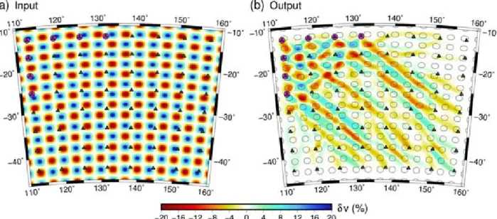
Below, we run a series of experiments using a purely synthetic data set; a similar set of experiments applied to ambient noise data recorded in Australia can be found in the Supplementary Information. The synthetic data set used here is based on a test model, source–receiver geometry and ray-path configuration shown

in Fig. 1. The pattern of velocity anomalies is randomly

gener-ated and exhibits a Gaussian distribution between peak values of

±20 per cent. Although this may seem large, there are many exam-ples of ambient noise surface wave tomography that recover peak perturbations in excess of 25 per cent relative to a background aver-age (e.g. Saygin & Kennett2010, and Supplementary Information). The design of the source–receiver array is such that there is good path coverage in the NW region of the model, but it gradually de-grades to the SE, where it becomes more unidirectional. This forms a good basis for assessing the characteristics of various synthetic recovery tests.

Fig.1(c) shows a reconstructed model based on inverting the true noise-free traveltimes associated with the paths shown in Fig.1(b). 20 iterations of the forward and inverse step were applied to obtained the solution, which corresponds to an RMS reduction in traveltime residuals from 18.4 to 0.35 s, at which point convergence is well and truly achieved (subsequent iterations had no appreciable ef-fect on the traveltime misfit). Minimal damping and smoothing was applied in this case as the implicit regularization imposed by the choice of basis function (cubic B-splines) was sufficient to stabilize

the inversion. A constant velocity model, set to the average velocity of the synthetic model, was used as the starting or initial model. Clearly, the reconstruction is best in the NW of Fig.1(c), but grad-ually degrades to the SE, where significant streaking effects can be observed, which can be attributed to the source–receiver geometry. Below, we use the experimental set-up of Fig.1to examine the characteristics of a variety of synthetic reconstruction tests. In each test, the reconstruction is carried out using the path coverage shown in Fig.1(d) (i.e. the path coverage associated with the output model), unless stated otherwise. Section 3.3 investigates what happens if a nonlinear method, in which rays are re-traced after every iteration, is used instead.

3.1 Checkerboard test

Fig.2(a) shows a checkerboard model comprising a fine-scale pat-tern of positive and negative anomalies, with peak values equal to those of the ‘observational’ model (Fig.1c). The sizes of the anomalies are approximately equal to the minimum scale-length of the structures present in Fig.1(a). If we use this checkerboard model as input, and compute a synthetic source–receiver data set by integrating along the path geometries of Fig.1(d), then we can solve the linear inverse problem to obtain the result shown in Fig.2(b); perhaps unsurprisingly, the checkerboard pattern is retrieved within the triangular region defined by the source geometry in the NW of the model but not elsewhere. A conventional interpretation of this figure might be that the NW sector of the model is quite well resolved, while the remainder of the model is poorly resolved, with a widespread tendency to smear structure in the NW–SE direction. Is this seemingly straightforward conclusion really borne out by the resolving power of the ray coverage?

3.2 Spike test

Fig.3(a) shows a spike model (or sparse checkerboard model) which has the same scale length and amplitude of anomalies as Fig.2(a), but is much more widely spaced. Fig.3(b) shows the result of ap-plying exactly the same inversion method that was used to derive Fig.2(b). Like before, the anomalies are most accurately recon-structed in the NW of the model, and generally become poorer to the southeast. However, when comparing Figs2(b) and3(b), there are a number of important differences. First, there is clear evidence of smearing towards the edges of the model for the most accurately recovered anomalies in the NW sector of Fig.3(b); in Fig.2(b), the distortion in the shape of the anomalies is much less apparent. Presumably, in the checkerboard model, this is due to the close proximity of adjacent anomalies, which tends to mask smearing effects that are not very major. Furthermore, in the southeast region of the spike model (Fig.3b), there is not the same dominance of NW-SE smearing, and it is now much clearer from the spike model how the anomalies are distorted as a result of the path coverage. In fact, we can now see that most anomalies experience some degree of recovery, even if their aspect ratios have changed from 1:1 in the input model to as much as 5-6:1 in the recovered model. This is useful information, not only on the level of distortion, but also the direction, and is entirely absent from the checkerboard result of Fig.2(b).

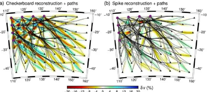
A comparison of the recovered anomalies in Figs2(b) and3(b) with the associated path coverage is shown in Figs4(a) and (b) re-spectively. The close proximity and regular pattern of the anomalies in Fig.2(a) mean that when path coverage is diagonally dominant,

(8)

Figure 1.(a) Synthetic test model and source–receiver geometry used for numerical experiments; (b) ray-path geometry through the synthetic model; (c) reconstruction of (a) obtained after application of the iterative nonlinear inversion scheme; (d) ray-path geometry through the recovered model. Dark grey triangles denote receivers and magenta circles denote sources.

the recovered anomalies do a reasonable job at fitting the traveltimes by smearing out in the diagonal direction, which is the direction in which we do not have an oscillation from positive to negative anomalies in the input model. By contrast, the spike test is able to better reveal the (lack of) resolving power of the ray illumination, and the recovery is hence more useful for interpreting directionally dependent solution smearing. For example, we see that the nega-tive anomaly at approximately (151◦E, 21◦S), which sits between receivers immediately to the west and to the east in Fig.3(a), is recovered as a horizontally smeared anomaly in Fig.3(b). The path coverage map in Fig.4(b) shows that this anomaly is crossed by a single horizontal ray, but just to the west, there is crossing path coverage, so the anomaly is represented by its path average approx-imation between the two stations. Another example is the negative anomaly at approximately (119◦E, 34◦S), which achieves a degree of recovery in Fig.3(b), but there is no evidence of recovery in the same region in Fig.2(b). Although the experiment set-up here is contrived, it is seems clear that the discrete spike test provides more useful information on spatial resolution from the

constrain-ing power of the path coverage than the equivalent checkerboard test.

In Section 2.3, the theory behind spike tests and their associa-tion with the resoluassocia-tion matrix was discussed. In effect, the input model of Fig.3(a) representsmsin eq. (16), while the output model

of Fig.3(b) represents ˆms, with the noise term set to zero, that

is,s =0. If the resolution matrixRwas available, then any input

model could be transformed into an output model. For this example, there are 3844 unknowns, which means that it is computationally feasible to calculateR. In general, this may not be the case, particu-larly for large 3-D problems. We solveR=G−g_G_{using Cholesky}

decomposition, which produces the complete 3844 ×3844

res-olution matrix. The compute time is approximately 12 min on a workstation equipped with an Intel Xeon 3.1 GHz E5-2687W

pro-cessor, 128 Gb of RAM and running Ubuntu 14.04. Fig.5compares

the spike test result of Fig.3(b) with ˆm∗_s =Rm∗_s, wherem∗_s is a se-lection of two anomalies from Fig.3(a). These two anomalies were chosen to be far apart so that any interference between their recon-struction is unlikely. It is clear that Fig.5(b) is essentially a subset

(9)

Figure 2. (a) Input checkerboard model; (b) recovered model using the path geometry of Fig.1(d). Black contour lines represent the±10 per cent contour interval of the input checkerboard.

Figure 3.(a) Input spike model; (b) recovered model using the path geometry of Fig.1(d). Black contour lines represent the±10 per cent contour interval of the input spikes. Closed dashed red lines highlight the locations of features discussed in the text.

of Fig.5(a); the very minor differences in recovery can be attributed to the fact that there is a small amount of smearing overlap between adjacent spikes. However, it is insignificant enough to ignore for interpretation purposes. The compute time needed to perform the Fig.5(a) spike test on the same computer was approximately 8 s,

which is two orders of magnitude faster than computingR. This

example demonstrates the power of well-chosen sensitivity tests: practical information on model resolution without the need to com-puteR. The checkerboard result of Fig.2(b) takes the same compute time as the spike test, but the overprinting of smearing effects from adjacent spikes makes it a less useful measure of model resolution.

3.3 Nonlinearity and the proper application of sensitivity analysis

In the above tests, the ray-path geometry (Fig.1d) is inherited from the observational model of Fig.1(c); this ensures that the synthetic

test provides information on spatial resolution that is consistent with the path coverage through the solution model. This is the same philosophy that is used to compute posterior model covariance and resolution for weakly nonlinear inverse problems (e.g. Tarantola 1987; Rawlinsonet al.2010).

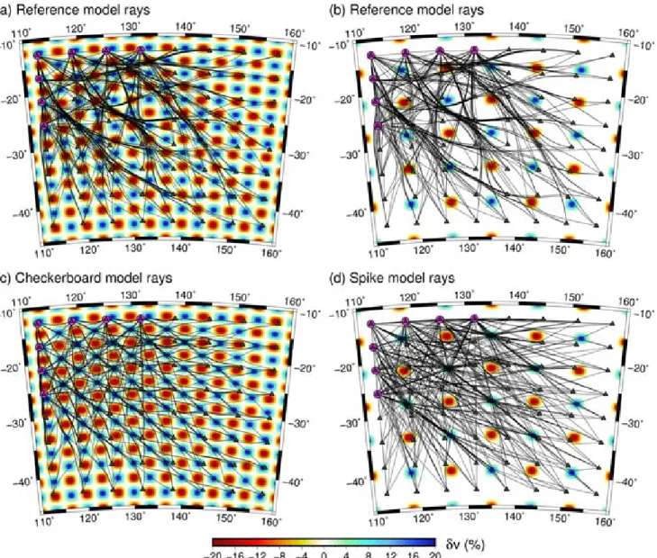
If instead the synthetic data set is computed by solving the full forward problem (ray tracing in this case) through the input model used for the synthetic test, and the input model is then recovered using an iterative nonlinear method which updates the ray paths, the result of the reconstruction can be quite different. Fig.6compares the true path coverage through the checkerboard and spike models of Figs2and3with the path coverage inherited from Fig.1(c). The differences are significant; in the case of the checkerboard model (Fig.6c) the paths are attracted to high velocity regions since only first arrivals are used. This is also true of the spike model (Fig.6d), although the path coverage is more even due to the increased spar-sity of model anomalies. The corresponding inversion results when

(10)

Figure 4.Comparison between path coverage and recovered structure for (a) checkerboard recovery of Fig.2(b); (b) spike recovery of Fig.3(b).

Figure 5.Comparison between sensitivity test and resolution matrix. (a) Spike test output from Fig.3(b); (b) resolution matrix multiplied by the true model

m∗s, wherem∗s consists of two spikes taken from Fig.3(a). In both (a) and (b), black contour lines represent the±10 per cent contour interval of the input

spikes.

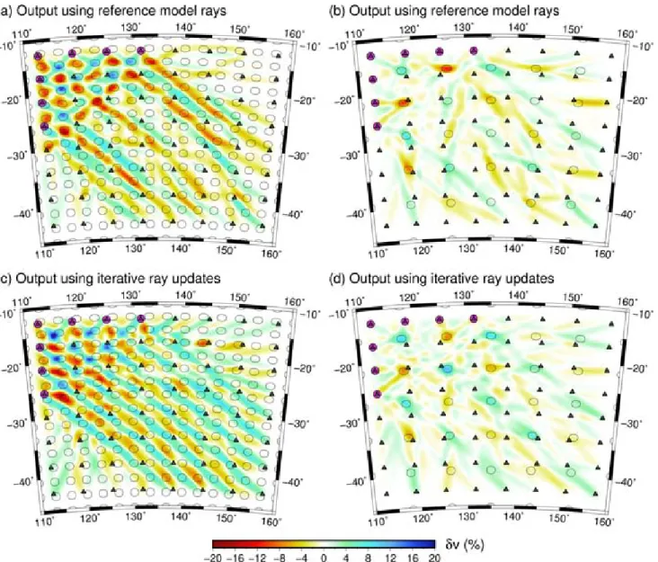
using these different sets of ray paths is clearly revealed in Fig.7. In the case of Figs7(c) and (d), the synthetic data set is created by inte-grating along the ray paths shown in Figs6(c) and (d) respectively. The output models are obtained by running the iterative nonlinear procedure until convergence is achieved. The checkerboard recov-ery in this case has far greater diagonal smearing compared to the linear inversion result of Fig.7(a), which uses the rays from Fig.6(a). This is partly due to the rays favouring the high velocity regions, which have an NW–SE orientation. There is also some hint of this in Fig.7(d), although it is less pronounced. The clear difference in results produced by this example means that it is important to use rays that are inherited from the original observational model as required by the theory (see point iv of Section 2.5), rather than rays traced through the synthetic test model, when the nonlinearity of the inverse problem is taken into account.

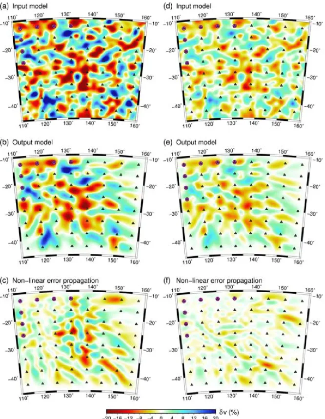
3.4 Nonlinear error propagation

In the previous section, we established the correct procedure for sensitivity analysis in the presence of weakly nonlinear inverse problems. However, it does not account for the effects of nonlinear error propagation, which remains an unsolved problem in synthetic testing. However, as was noted in Section 2.4, we can investigate nonlinear error propagation for a purely synthetic experiment by evaluatingE=G−Gs, whereGs is computed from the true (or

input) model andGis computed from the reconstructed (or output) model. This allows the error propagation termG−g_Em

pin eq. (18)

to be computed, thus providing quantitative insight into the influ-ence of nonlinearity. Fig.8shows the result of this analysis in the presence of our default test model (shown in Figs1a and8a), and a model which exhibits an identical pattern of anomalies but with

(11)

Figure 6. Path coverage through checkerboard (left column) and spike (right columns) models from Figs2and3, respectively. (a), (b) show the path coverage inherited from the recovered model shown in Fig.1(d), while (c), (d) show the path coverage obtained by solving the forward problem through the checkerboard and spike model respectively.

reduced amplitude (Fig.8d). In the case of the original test model, the magnitude of the error is smallest in the NW portion of the model where there is both good path coverage and relatively short paths in comparison to the dominant wavelength of the velocity anomalies. The errors tend to peak in the central and SE region of the model, where path density is still moderate, but paths are on av-erage longer and angular covav-erage is poorer. Overall, the magnitude of the error is smaller than the amplitudes of the recovered anoma-lies (cf.Figs8b and c), particularly in the well resolved region in the NW.

If we now decrease the amplitudes of the input anomalies by 50 per cent (Fig.8d), the effect of the nonlinear error propagation is much reduced (Fig.8f), which is consistent with solving a more linear inverse problem. Our results indicate that even in the pres-ence of sizable anomalies (up to 20 per cent) the weakly nonlinear assumption can be valid (cf.Figs8a and b), and in regions of good angular path coverage, the nonlinear propagation error can be small relative to the amplitude of the recovered anomalies.

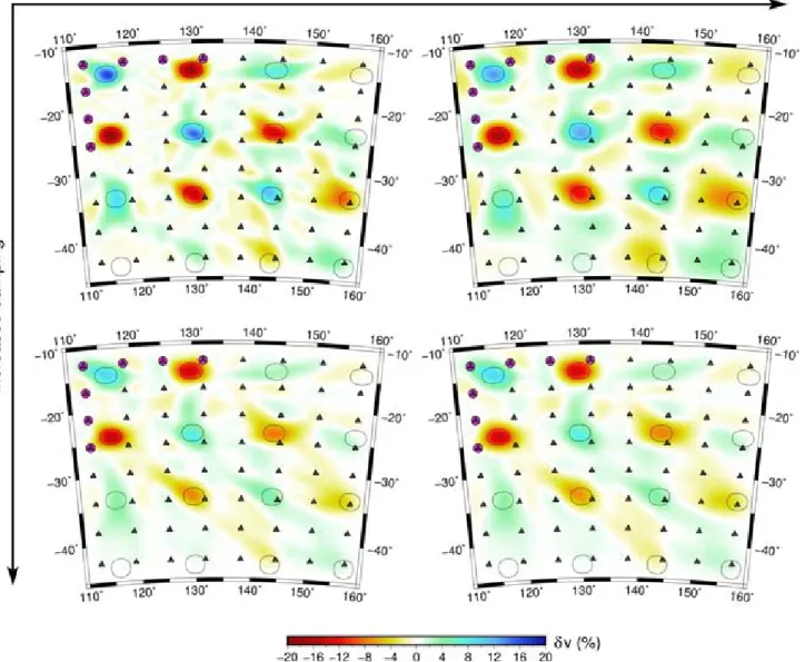
3.5 Using various test models with difference scale lengths

One problem with using a single checkerboard or spike test with only one scale length of structure is that it does not necessarily reveal resolution artefacts over multiple scales. Moreover, as demonstrated by L´evˆequeet al.(1993) (see Section 2.5, point ii), there are certain specific circumstances in which the common expectation that the region of good recovery increases in size as the scale length of struc-ture increases is not always a given. Therefore, it may ultimately be misleading to present the result of a single spike or checkerboard test to assess lack of resolution. We illustrate scale dependence in Fig.9, which shows the results of performing the same inversions as Figs2and3, but now with much broader anomalies. In this case, both the checkerboard and spike anomalies have much improved re-covery (in shape and amplitude) compared to the previous test. This is consistent with the Fig.1test, in which the broader scale anoma-lies are more accurately retrieved than the smaller scale anomaanoma-lies. These results illustrate that, at least in this case, larger structures

(12)

Figure 7.Checkerboard (left column) and spike (right column) output models based on different path coverage. (a), (b) are the result of a linear inversion using rays from the Fig.1(d) model. (c), (d) are the result of an iterative nonlinear inversion in which rays are updated for the model obtained after each iteration.

are more easily resolved than smaller structures with the same path coverage.

Fig.9also helps to reinforce the point that spike tests are more useful than checkerboard tests in providing insight into the ability of a rayset to resolve structure and reveal directional dependence in resolution artefacts. Even though, as a result of the presence of longer wavelength anomalies, the recovery of equivalent anomalies between Figs9(c) and8(d) show greater similarity than between Figs2(b) and3(b), the full extent of smearing is more successfully revealed in Fig.9. For example, the positive anomaly at approxi-mately (116◦E, 33◦S) shows much less distortion in the N–S di-rection in Fig.9(c) than in Fig.9(d), and the positive anomaly at approximately (143◦E,14◦S) shows much less E–W distortion in the output checkerboard model. Both of these effects can be attributed to the close proximity of anomalies of opposite sign.

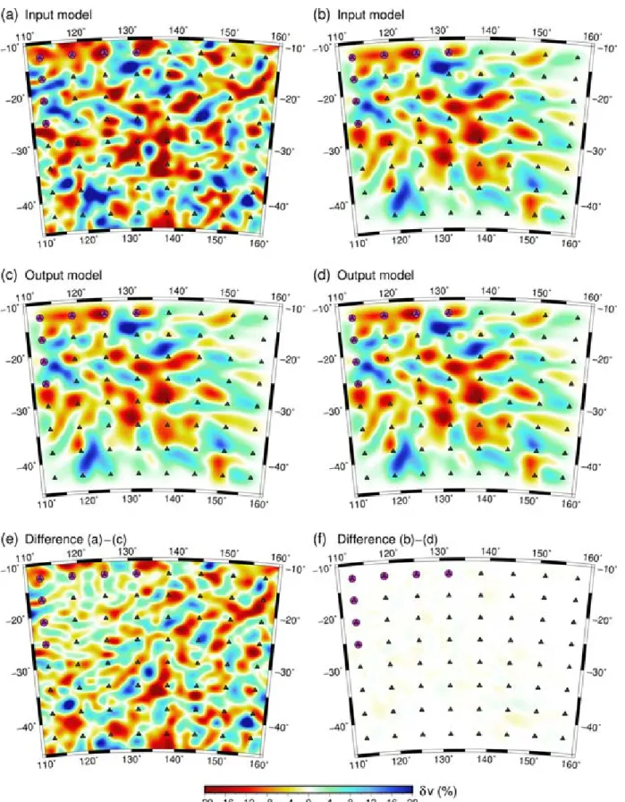
3.6 Synthetic test based on observational model

As well as synthetic tests involving anomalies of a fixed scale-length, it is relatively common to find studies that use a test

struc-ture that bears some resemblance to a geological feastruc-ture such as a subducting slab (e.g. Spakmanet al.1989; Eberhart-Phillips & Reyners1997; Bijwaardet al.1998; Graeber & Asch1999; Wolfe

et al.2002). While this kind of hypothesis testing is reasonable, it is important that the synthetic model does not too closely resemble what has been recovered from the observational data set, as was pointed out in Section 2.5, point vii. Fig.10compares the result of the recovery test shown in Fig.1with a new test that uses the model shown in Fig.1(c) as the input test model (i.e. the output model of Fig.1a). It is clear that the model recovered in this case is almost identical to the input model (see Fig.10f), confirming what is ex-pected from theoretical considerations (Section 2.5, point vii). This result stands in stark contrast to Fig.10(e), which shows the differ-ence between the original synthetic model and its reconstruction. Although this is a somewhat extreme example, it does demonstrate the point that care needs to be taken in the choice of synthetic test model used.

Tests based on the observational model should concentrate on detecting lack of resolution e.g. by setting parts of the model to zero perturbation and inferring from the sensitivity tests what is being

(13)

Figure 8. Test results illustrating the influence of nonlinear error propagation in the solution. Left column uses the same input model as in Fig.1, while the input model for the right column has an identical pattern of anomalies but with a 50 per cent reduction in amplitude. (a), (d) Input model; (b), (e) output model from iterative nonlinear inversion; (c), (f) estimate of nonlinear error propagation as given by the termG−gEmpin eq. (18).

mapped in these regions due to a lack of resolution. For example, will a short slab produce a long slab (Spakmanet al.1989); will a layer-cake slab produce a continuous slab (Bijwaardet al.1998); will a layer-cake plume produce a continuous plume (Bijwaard &

Spakman1999)?

3.7 Testing the influence of explicit regularization

Explicit regularization in the form of damping and/or smoothing will invariably influence the recovery of structure, as shown in Fig.11. Clearly, in performing a synthetic test, one should use the

(14)

Figure 9.Synthetic recovery test involving larger anomalies. (a) Input checkerboard model; (b) input spike model; (c) output checkerboard model; (d) output spike model. Compared to the equivalent tests displayed in Figs2and3respectively, the anomalies are approximately four times the size. Black contour lines represent the±10 per cent contour interval of the input anomalies. Closed red dashed lines denote the location of anomalies discussed in the text.

identical regularization that is chosen for the observational data. The sensitivity of the solution to model regularization can also be tested using sensitivity analysis with the aim of converging to optimal settings of regularization and model parametrization. This would involve tests similar to those used for assessing resolution and noise propagation for the final observational model: (i) noise-free tests covering a range of length scales combined with (ii) various noise tests such as the permuted data test (Section 2.5, point vi). In addition, these tests can be conducted for various levels of detail in the model parametrization. If one converts the outcome of such tests into a scalar measure of local resolution this can be used as input for optimizing strategies for the design of spatially variable model parametrization (e.g. Spakman & Bijwaard2001) that are adapted to the expected resolution.

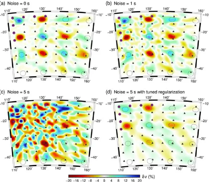
3.8 The influence of data noise

Data noise is ubiquitous to all seismic data sets, but in most cases the magnitude and distribution of this noise is poorly understood,

as noted previously. Synthetic recovery tests are either noise free to assess optimal spatial resolution or include noise with a Gaus-sian distribution and standard deviation equal to that of noise es-timates obtained from the data such as picking error (Rawlinson

et al. 2014). Spakman & Nolet (1988) advocate the addition of synthetic noise such that a data fit is obtained similar to that of the real data inversion. Although both approaches appear to be rea-sonable, estimating data uncertainty is notoriously subjective, and there is often little evidence that the actual noise distribution is Gaussian. To partially mitigate this, one can apply permuted data tests, which randomize the data vector prior to inversion in order to investigate the propagation of more realistic noise (Spakman & Nolet1988). Another potential issue is that the use of an L2 norm in most inversion schemes is not robust in the presence of noise with a non-Gaussian distribution (Parker1994), which may also cloud the results.

Sensitivity tests can be used to study the effects of various noise levels on the solution. The Fig.12example is the same as the Fig.3 example but now includes varying levels of Gaussian noise. As

(15)

Figure 10. Left column: synthetic recovery test from Fig.1; right column: synthetic test which uses the recovered model (c) of the left column test as the input model for a new test. (e) and (f) show the difference between the input and output models for both tests.

expected, increasing the noise level degrades the quality of the re-construction. However, as Fig.12(c) shows, if explicit regularization is not applied, then the inversion will attempt to overfit the data and spurious structure is introduced. If instead the simplest model

(ob-tained using smoothing and damping) is found that fits the data, then the more robust elements of the model are recovered. One of the challenges in using the standard deviation of the noise as a measure of fit (as in theχ2_{test) is that this value is often poorly constrained.}