Implied Volatility and the Cross Section of Stock Returns in the UK
Sunil S. Poshakwale1#, Pankaj Chandorkar2and Vineet Agarwal3 1Professor of International Finance
Director of Centre of Research in Finance
Cranfield School of Management, Cranfield University, England – MK43 0AL Phone: +44 (0) 1234 754404, e-mail: [email protected]
2Lecturer in Finance:
Northumbria University, Newcastle Business School Department of Accounting and Financial Management
City Campus East, Newcastle upon Tyne,
NE1 8ST
Email: [email protected]
3Reader in Finance
Centre for Research in Finance, Cranfield School of Management, Cranfield University, England – MK43 0AL
Phone: +44(0)1234 75112, email: [email protected]
#Corresponding author
Research in International Business and Finance, Volume 48, April 2019, pp. 271-286 DOI:10.1016/j.ribaf.2019.01.006
Implied Volatility and the Cross Section of Stock Returns in the UK Abstract
The paper examines the relationship and the cross-sectional asset pricing implications of risk arising from the innovations in the short and the long-term implied market volatility on excess returns of the FTSE100 and the FTSE250 indices and the 25 value-weighted Fama-French style portfolios in the UK. Findings suggest that after controlling for valuation, macroeconomic, leading economic and business cycle indicators, returns exhibit a strong negative relationship with the innovations in both the short and the long-term implied market volatility. The cross-sectional regression provides new evidence that changes in both short and long-term implied market volatility are significant asset pricing factors with negative prices of risk, which suggests that (i) investors care about ex-ante volatility and (ii) they are willing to pay for insurance for future uncertainty.
Keywords: VFTSE, Excess Returns, Asset Pricing, Business Cycle, ICAPM, implied volatility
1.0
Introduction
There is a long-standing academic interest in investigating the relation between market volatility and stock returns. Broadly speaking, there are two groups of literature, which deal with this issue. First, group investigates this relationship using realised or ex-post volatility [see for example, French, Schwert, and Stambaugh (1987), Schwert (1989a), Bae, Kim and Nelson, (2007)]. Second group deals with this issue using short-term implied volatility. Since investors are mostly concerned about ex-ante risk, implied volatility rather than realised volatility is considered as a better measure of risk for determining stock returns. For example, Ang, Hodrick, Xing and Zhang (2006) show that aggregate market volatility implied by the VIX index is a key factor in explaining the cross-section of expected returns. Bollerslev, Tauchen and Zhou, (2009) show that the difference between “model-free” implied variance (squared VIX index) and the realised variance significantly explains the variations in expected stock returns. Further, Drechsler and Yaron (2011) show that the variance risk premium, the difference between squared VIX index and the conditionally expected realised variance, is linked to the underlying economic volatility and can predict future stock market returns. Finally, Lubnau and Todorova (2015) analyse the predictive ability of short term implied market volatility in forecasting stock returns. Their findings suggest that periods of low volatility are followed by significant positive mean returns over 20, 40 and 60 trading days.
Although the extant literature has examined the empirical link between short-term implied volatility and stock returns, it overlooks the impact of long-term implied volatility. Investors are not only concerned about short-term volatility but they are equally apprehensive about the likely impact of the longer-term volatility on stock returns. Indeed, market volatility is driven by the changes in macroeconomic variables and therefore can capture business cycle risk (Schwert, 1989a; Schwert, 1989b). Consequently, it is critical to investigate whether asset
also with the factors which drive volatility of future investment opportunity set in the long-term. Furthermore, such an investigation is absent in the context of the UK stock market as most of the studies mentioned above use the US data. It is worth conducting such an investigation in the context of the UK Stock market as recent idiosyncratic events such UK’s exit from the European Union (“Brexit”) and the ensuing political and currency crisis could affect long-run volatility of future investment opportunities in the UK.
Against this backdrop, this paper makes two novel contributions to the existing literature. First, the paper investigates the extent to which both the short and the long-term implied market volatility drive the UK stock returns. Secondly, the paper offers new insights on the asset pricing implications of the risks arising from innovations in both the short and the long-term implied market volatility.
This paper is similar to the work of Adrian and Rosenberg, (2008) which considers the impact of short and long-term conditional market volatility on US stock returns. They decompose the conditional volatility of market returns into short and long-term to capture the financial constraints and business cycle risks respectively. They find that both short and long-term volatility are negatively priced. However, this paper is vitally different from Adrian and Rosenberg, (2008) as the focus is on changes in the expected short-term (30-days) and long term (360-days) model-free implied market volatility. Implied volatility is both observable and free from estimation bias. Contrary to this, Adrian and Rosenberg, (2008) use conditional market volatility which is not only unobservable but is also subject to estimation bias since it depends on the type of time-series model employed for its estimation. [See for example: Heynen, Kemna and Vorst, (1994), Dumas, Fleming and Whaley, 1998)]
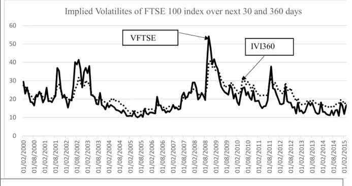
We use the VFTSE volatility index and the FTSE 100 interpolated annualised Implied Volatility Index (IVI360) as proxies of short term and long-term implied market volatility
respectively. Similar to the Chicago Board of Exchange’s VIX index, the VFTSE represents the risk-neutral expectation of market participants about the future market volatility of the FTSE 100 index over the next 30 calendar days. Similarly, the interpolated FTSE IVI 360 index represents market participants’ risk-neutral expectations about future market volatility over next one year. Both VFTSE and IVI360 are constructed using the collection of out-of-money put and call options on the FTSE 100 index using appropriate maturities which represent “model-free” measures of implied market volatility.1
There is extensive support in the literature for using “model-free” measure of implied volatility. Jiang and Tian (2005) show that option implied volatility is immune from model misspecification errors and is informationally superior. Dennis, Mayhew and Stivers (2006), suggest that systematic volatility, measured using implied volatility has a bigger impact on stock returns than idiosyncratic volatility. Banerjee, Doran and Peterson (2007) also lend support to using model free implied volatility as they find both current and future innovations in the implied volatility are useful in predicting future excess returns. Besides the rationale offered by academic research, the Bank of England (BoE) also considers implied volatility as one of the indicators of future economic uncertainty.2
We study the impact of the short term and the long term implied market volatility by using returns on the FTSE 100 and FTSE 250 indices in excess of the one-month UK Treasury-bill rate while controlling for a variety of variables. We use the following control variables found in the literature as useful for predicting the stock market returns3. The first group of
control variables includes valuation ratios i.e., dividend yield, price-to-earnings ratios and
1For more information regarding the construction methodology of the FTSE Implied Volatility Index follow
this link http://www.ftse.com/products/downloads/FTSE_Implied_Volatility_Index_Series.pdf
market liquidity. The second group comprises eight UK macroeconomic indicators i.e., inflation, unemployment, narrow and broad money supply, effective exchange rate, the term spread (measured as the difference in the yields of UK 10 year Government bond and 3-month Treasury-bill) and the short-term transitory deviations between consumption, asset wealth and income (CAY). The third group of control variables includes leading economic indicators i.e., changes in the retail sales, industrial production, consumer confidence and the composite leading indicator. We also study the asset pricing implications of the risk associated with the changes in the short and long term implied market volatility in the cross-section of excess returns of twenty-five Fama-French portfolios sorted on size and book-to-market characteristics ( Fama and French 1992).
Using data from February 2000 to June 2015, we find that the innovations in both the short and long-term implied market volatility have a significant negative impact on the excess returns after controlling for valuation ratios, macroeconomic and leading economic indicators. Notably, we find that the excess returns from FTSE 250 index are more sensitive to the innovations in both the short and the long-term implied market volatility as compared to the FTSE 100 index. Furthermore, we find that the excess returns from both FTSE indices are more sensitive to the innovations in the long-term implied market volatility, which imply that investors seem more concerned about the long-term uncertainty.
The cross-sectional analysis using 25 Fama-French style portfolios, sorted on size and book to market characteristics shows that the impact of changes in the short (long)-term implied market volatility has positive (negative) impact on the excess returns of small size portfolios after controlling for the market risk premium. This suggests that investing in small size portfolio may provide a hedge against the short-term market uncertainty. In contrast, investing in large stock portfolio seems to provide a better hedge against the longer-term implied market volatility. Overall, the 25 Fama-French portfolios show greater sensitivity to the changes in the
long-term implied market volatility. We find evidence of cross-sectional pricing ability of both the short and the long-term implied market volatility after controlling for popular cross-sectional asset pricing factors such as market, size, value, momentum premiums and variety of business cycle variables.
We test the robustness of our results in two different ways. First we measure the innovations in the VFTSE and IVI360 indices by using; (i) changes in these indices, (ii) innovations from ARMA (1,1) model and, (iii) orthogonalised innovations of VFTSE and IVI360 indices by regressing them on variety of business cycle and macroeconomic indicators. Second, we re-estimate our models using the Generalised methods of Moments (GMM) specifications.4We find that our results remain robust and confirm our findings that the short
(long)-term implied volatility positively (negatively) affects excess returns and changes in both the short and the long-term implied market volatility are significant asset pricing factors with negative prices of risk. This suggests that (i) investors care about ex-ante volatility and (ii) they are willing to pay for insurance for future uncertainty.
The remainder of the paper is organised as follows; section 2 describes the theoretical motivation and the empirical approach used in the paper. Section 3 describes the data. Section 4 reports and discusses empirical results. Section 5, reports results of robustness tests and section 6 concludes.
2.0 Theoretical motivation and methodology
2.1 Theoretical motivation
The Intertemporal Capital Asset Pricing Model (I-CAPM) of Merton (1973) and the Arbitrage Pricing Theory (APT) of Ross (1976) postulate that when an investor’s future opportunity set is stochastic, asset risk premia are proportional to the covariation of asset
returns with systematic factors in addition to the market factor. Further, the stochastic discount factor is a function of innovations in other systematic state variables that can drive investor’s opportunity set. Campbell's (1993) version of I-CAPM shows that under the assumption of homoscedastic environment, investors care about future expected news, which implies that excess stock returns are proportional to the covariance of asset returns with news influencing future market returns. Chen (2002) extends Campbell's (1993) version of I-CAPM under the assumption of heteroscedasticity and time-varying conditional co-variance of asset returns with stochastic discount factor. He shows that investors care about expected volatility and so they like to hedge risk arising from the future innovations in the volatility.
Motivated by these theoretical implications of the I-CAPM, we hypothesise that the short and the long term implied market volatility will affect investors’ short and long-term opportunity set thus driving the risk premium they demand to offset risk. Further, these risk factors should be priced in the cross-section. Thus, we use 30 days and 360 days implied market volatility for explaining returns using the following model:
, = ,. , , + , . , , + ,. , , (1)
where , is the expected excess return on risky asset, is the short term implied market volatility (30 days) and is the long term implied market volatility (360days). are the respective prices of risks.
2.2 Methodology
In this section, we describe our empirical approach. We begin our analysis by studying the impact of risk associated with the changes in the short term (VFTSE) and the long-term implied market volatility (IVI360) on the excess returns of aggregate FTSE indices. For this, we estimate the following regression;
= + .Δ , + .Δ , + . + (2) where, is the excess returns of the FTSE index i,Δ , is the change in the short term implied market volatility (VFTSE index), Δ , is the changes in the long term implied market volatility, represents control variables and is the error term which is assumed to follow a white noise process. and capture the sensitivities to changes in the short and the long term implied market volatility. As mentioned earlier, we use three groups of control variables; three valuation metrics, eight macroeconomic indicators and four leading economic indicators separately. With these sets of control variables, model (2) is modified as:
= + ∆ , + ∆ , + + . + . , + (2a)
where, is the dividend yield of the ithFTSE index, is the Price-Earnings ratio ofith
FTSE index and the is the log of trading volume which is our measure of market liquidity. Gervais, Kaniel and Mingelgrin (2001) show that trading volume contains important information about the future stock returns. Periods of excessive trading are followed by high stock returns and periods of low trading volume are followed by low stock returns. They refer to this phenomenon asHigh Volume Return Premium.
With the second group of control variables model (2) becomes,
= + ∆ , + ∆ , + . + . + ∆ 0 + ∆ 4 + ∆ + Δ
+ +
(2b) where, is the inflation, is unemployment rate, ∆ 0 log changes in the narrow money supply (M0),∆ 4is the log changes in the broad money supply (M4),∆ is the log changes in the Sterling’s effective exchange rate index, ∆ is the changes in the term spread measured as the difference between the yields on the 10 year and the 3-month UK Treasury-bill. Following Lettau and Ludvigson (2001), we also control for the transitory deviations between
the consumption, asset wealth and income, (CAY). We construct theCAYvariable as residuals of the following cointegrating regression;
= + . + + (3)
where, is the log of aggregate household consumption in the UK, is the log of aggregate household wealth and is the log of aggregate disposable household income. =CAYis the transitory deviation between these three variables. We estimate this cointegrating regression by dynamic OLS5
Finally, with the third set of control variables, model (2) becomes
= + ∆ , + ∆ , + ∆ + .∆ + . + ∆ + (2c)
where, ∆ is the log changes in the retail sales, ∆ is the log changes in the Index of Industrial Production, is the changes in the consumer confidence index and∆ is the log changes in the composite leading indicator.
We investigate the cross-sectional asset pricing implications by using twenty-five Fama-French size and book-to-market portfolios. For this we employ the two-stage Fama and MacBeth (1973) cross-sectional regression approach. In the first stage we run the following time-series regression;
= + 30∆ 30, + 360∆ 360, + . + (4)
where, represents the excess returns of the pth size and book-to-market portfolio at timet,
is the excess market return at time t (Market Factor). The respective coefficients represent the loadings of the excess returns of thepthsize and book-to-market portfolio on the
respective factors. In the second stage, we use cross-sectional regressions to estimate the price
of risk arising from changes in the short term and long term implied market volatility. For this purpose we estimate following cross-sectional regressions;
= + + . + . + (5)
= + + . + . + . + . + . + (6)
where, represents the excess returns of the pth size and book-to-market portfolio, and
represent the unconditional prices of risk arising from the exposure to changes in the short term and the long term implied market volatility. In cross-sectional regression (5) the are estimated from time series regressions (4). We augment model (5) by including the exposures to size premium (SMB) and value premium (HML) of Fama and French (1993) and momentum factor (UMD)of Carhart's (1997) model. Thus, in model (6) , and denotes the time-series loadings on size, value and momentum premiums and , and are corresponding factor premiums respectively. Models (5) and (6) are estimated using Newey and West (1987) (Heteroscedasticity and Autocorrelation Corrected) standard errors. In addition to controlling for the Fama and French (1993) and Carhart's (1997) factors, we also control for seven economic indicators, used previously, in investigating the impact of changes of short and long term implied market volatility on the excess returns of the aggregate the FTSE indices. Thus, we estimate the following cross-sectional regression model:
= + + . + + + + . + . + .
+ . + . +
(7) where, , , , , , , and are the prices of risk associated with exposure to market risk premium, inflation, unemployment, changes in narrow money supply, changes in broad money supply, changes in Effective Exchange Rate, changes in the term spread and theCAYrespectively.
For ensuring that our results are robust, we use residuals from ARMA (1, 1) model and orthogonalised innovations to VFTSE and IVI360 indices as proxies of innovations in the short and the long term implied volatility. We use the Akaike (1973) Information Criteria for selecting the lags and use the ARMA (1, 1) residuals and re-estimate models (5), (6) and (7).
3.0 Data Description
We estimate ex-post excess returns for the FTSE 100 and FTSE 250 indices using the total return index, which includes dividends less the one-month T-bill rate. We use the VFTSE and FTSE interpolated 360 days volatility indices (IVI360) as a proxy of short-term and long-term implied volatility. We obtain data on total return indices and control variables from DataStream and Bloomberg6. A brief description of the control variables is given in Table A1 of Appendix A.
We obtain returns on the twenty-five Fama-French style portfolios based on size and book-to-market characteristics from Gregory, Tharyan and Christidis (2013).7 Data for size
premium (SMB), value premium (HML) and the momentum factor (UMD) are also taken from the same source. The market risk premium (MKT) is calculated as the difference between the total return on the FTSE All Share Index and the one month treasury-bill rate. Data are obtained at monthly frequency for the period February 2000 to July 2015 since the FTSE IVI 360 index is available only from the year 2000.
Figure 1 shows the VFTSE and FTSE IVI 360 day indices. The thick line represents the implied volatility over the next 30 days (VFTSE index) and the dotted line shows implied volatility for the next 360 days (IVI360). For most periods, the long-term implied volatility is higher than the short-term implied volatility. However, as would be expected, during the
6Bloomberg ticker for the 30 days and 360 days implied volatility are VFTSE and IVUKX360 respectively 7http://business-school.exeter.ac.uk/research/centres/xfi/famafrench/
financial crisis in September and October 2008, the short term implied volatility is much higher than the long-term implied volatility.
***please insert figure 1 about here***
Panel A of Table 1 provides the descriptive statistics. The average monthly short and long term implied market volatility of the FTSE 100 index is 20.19% and 21.68% with standard deviation of 8.00% and 5.66% respectively. Panel B provides the annualised descriptive statistics of the ex-post excess returns of the two aggregate FTSE indices. The average annual excess returns of the FTSE 100 and the FTSE 250 indices are 0.89% and 6.75% with standard deviation of 14.23% and 17.70% respectively. The excess returns from largest 100 UK listed firms are notably lower than the smaller size firms represented in the FTSE 250 index for the sample period. Panel C provides the annualised descriptive statistics of the four well-known cross-sectional asset-pricing factors. We can notice that the momentum premium is the highest of all the pricing factors. This suggests that an investor would have earned an average of 9.54% by investing in a portfolio, which is long “winners” and short “losers” based on past 12 month’s returns.
Panel D presents the descriptive statistics of the macroeconomic indicators. The average annual growth rate of narrow money is 5.46% whereas the average term spread is about 0.99%. Interestingly, the average annual effective exchange rate of -0.69% shows that on average the value of Sterling has fallen against the basket of currencies of major trading partners of the UK. Panel E provides the descriptive statistics of the leading economic indicators. The average annual change in the retail sales is 2.24% while the average annual change in the index of industrial production is -0.75% indicating that industrial production has decreased. Finally, Panel F provides descriptive statistics of the valuation ratios such as PE ratios and dividend
yield of each of the FTSE indices. Average dividend yield of FTSE 100 index (3.32%) is greater than that of FTSE 250 index (2.76%).
***please insert table 1 about here***
4.0 Results
In this section, we present the results of our analysis. We first examine the impact of innovations in the short and the long-term implied market volatility on excess returns of aggregate FTSE indices. We then report the cross-sectional asset pricing using the 25 size and book-to-market portfolios.
4.1 The impact of the short and the long-term implied market volatility
Table 2 reports the impact of ∆ and ∆ on the excess returns of FTSE 100 and FTSE 250 indices. Panels A, B and C report the impact after controlling for macroeconomic indicators, leading economic indicators and valuation indicators, respectively. The results show that changes in both short and the long-term implied market volatility significantly affect excess returns. The impact is negative which suggests that an increase in the implied market volatility adversely affects stock returns. These findings are consistent with Black, (1976), Christie, (1982) and Schwert, (1989b) and suggest that increased implied volatility indicates increased future financial uncertainty causing negative market returns.
***please insert table 2 about here***
Panel A shows that the absolute impact of changes in the long term implied market volatility is higher for the FTSE 250 than the FTSE 100 index. This suggests that the FTSE 250 is more sensitive to the risk associated long-term implied market volatility after controlling for macroeconomic indicators. Results in Panel B and Panel C are also consistent with results in Panel A. However, the impact of∆ and ∆ on FTSE 100 is almost similar.
We also assess the impact of ∆ and∆ on the excess returns of aggregate FTSE indices in presence of all control variables together. Panel A of table 3 reports the results and shows that after controlling for a variety of the leading economic variables and valuation ratios, the impact of risk associated with changes in both the short term and the long term implied market volatility is significantly negative. The FTSE 100 excess returns are slightly more sensitive to changes in short-term implied market volatility than long term implied market volatility (| |= 0.48 >| |= 0.37), whereas for the FTSE 250, the changes in long term implied market volatility have a larger impact (| |= 0.61) than changes in the short term implied market volatility (| | = 0.49). For ensuring that our results are robust, we use residuals obtained from ARMA (1, 1) model as proxies of innovations in the short and long-term implied market volatility. Results in Panel B confirm that the changes in both short and long term implied market volatility have a significant negative impact on excess returns.
***please insert table 3 about here***
4.2 Cross-sectional excess returns and prices of risk
In this section, we analyse the impact of risk associated with changes in the short and the long-term implied market volatility on the excess returns of the 25 size and book-to-market Fama-French portfolios while controlling for the market factor. Subsequently, we estimate the prices of risk associated with exposure to ∆ and∆ in presence of the cross-sectional asset pricing factors.
***please insert table 4 about here***
Table 4 reports the estimations using model (4). The results show that the average impact of the short term implied market volatility on excess returns of the size portfolios decreases as one moves from small to large size portfolios. The average impact of ∆ on small size
portfolios provide higher risk adjusted excess returns. This is consistent with the findings reported by Pastor and Veronesi (2003) who show that the uncertainty related to future profitability of small stocks is much higher than large stocks which explains why small stocks provide higher risk adjusted returns. Further, Adrian and Rosenberg (2008) also report higher average exposure of small stocks to short term conditional market volatility.
Across the value dimension, the impact of risk associated with changes in the short-term implied market volatility increases as one moves from growth to value portfolios. On average, the impact of∆ on the excess returns of growth stocks is 0.05 as compared to 0.21 for the value stocks. Growth stocks provide less insurance against the risk of short term implied market volatility than the value stocks.
As far as the impact of risk associated with changes in the long term implied market volatility is concerned, we find that, on size dimension, small stocks are significantly more sensitive to∆ . The average impact of∆ on the excess returns of small size portfolios is higher (-0.66) than for the large size portfolio (0.16). On average, the large stocks provide positive risk-adjusted excess returns to offset increase in the long term implied market volatility. These results are qualitatively similar to Adrian and Rosenberg (2008) who also find that average loadings on the long term conditional market volatility for large stock returns are higher compared to the small stocks.
Further, the growth stocks show greater sensitivity to changes in the long-term implied market volatility than the value stocks. However, similar to the impact of the short-term implied market volatility, the average magnitude of impact of long term implied volatility on the excess returns of value stocks is larger than the growth stocks (|−0.45| > |−0.13|).
Column 1 of Table 5 presents the results of Fama and MacBeth (1973) cross sectional regression as per equation (5), whilst Column 2 shows the results of regression using equation
(6) which controls for the size, value and momentum premiums. The aim is to examine the pricing of∆ and∆ in presence of the market factor as well as the Fama-French (1993) and Carhart (1997) factors. The t-statistics are estimated using the Newey and West (1987) standard errors accounting for heteroscedasticity and autocorrelation.
***please insert table 5 about here***
The results of cross-sectional regression show that the prices of the risks of both the short-term and the long-short-term implied market volatility are negative and statically significant (-1.95% and -1.30% respectively) after controlling for the market risk premium. The negative prices suggest that when the short and the long-term implied market volatility are high, assets with high returns are expensive and consequently have low expected returns. The price of risk of -1.95% implies that assets which have unit exposure to the short-term implied market volatility will have 1.95% lower excess returns than the asset with zero exposure. Similarly, the price of risk of -1.30% means that assets with unit exposure to the long-term implied market volatility risk will earn 1.30% lower excess returns than the an asset with zero exposure. Our results are consistent with both Ang et al. (2006) who report negative prices of risk as implied by the VIX index and Adrian and Rosenberg (2008) who show that the short and long-term conditional volatility is negatively priced. From Column 2, a similar interpretation can be made after controlling for the size, value and momentum premiums in addition to the market risk premium. The prices of both short and long-term implied market volatility remain negative and statistically significant at 1% level.
In columns (3) and (4) of table 5, we check the robustness of our results in columns (1) and (2) by using the residuals of ARMA (1,1) models, which proxy for innovations in the short and the long-term market volatilities. We do not present the first stage factor loadings (betas)
cross sectional regressions in equations (5) and (6) using the betas of ARMA (1, 1) residuals. Results in columns (3) and (4) show that the pricing of both short and long-term implied market volatility remain negative and statistically significant confirming our results reported in columns (1) and (2) respectively.
***please insert table 6 about here***
In Table 6 we report the expected factor risk premiums for each of the 25 Fama-French portfolios. Factor risk premiums are calculated by multiplying the factor loadings from table 4 with prices of risks from column 1 of table 5. Panels A and B show the factor risk premiums attributable to the exposure to changes in the short-term and the long-term implied market volatility, while Panel C reports factor risk premium attributable to the market factor. The average risk premium of large stocks attributable to changes in the short term implied market volatility is positive (0.11% monthly) while the average risk premium of small stocks is negative (-0.44% monthly). On the other hand, the risk premium due to exposure to the changes in the long-term implied market volatility for large stocks is negative (-0.21% monthly) while it is positive for the small stocks (0.86% monthly). This is because the magnitude of factor loadings for small stocks is larger. Moreover, the risk premium of the 25 portfolios attributable to both the implied market volatility components is greater than the risk premium for the exposure to the market risk. For example, the risk premium for small stocks attributable to combined implied market volatility components is 0.42% monthly (0.86% + (-0.44%)) which is greater than that attributable to market risk premium (0.15% monthly). Overall, the average monthly risk premium for all portfolios attributable to the risk of changes in the short and the long-term implied market volatility is -0.19% and 0.45% respectively implying that investors will expect to earn positive risk premium for the risks associated with changes in the long-term implied market volatility.
4.3 Pricing implications in presence of business cycle indicators
In the previous section, we examined the pricing implications of exposures to the short and the long-term implied market volatility in presence of well-known cross-sectional asset pricing factors. In this section, we extend our analysis by including business cycle indicators. Schwert (1989a) show that business cycle is an important driver of market volatility. Further, Lettau and Ludvigson (2001) find that introduction of macroeconomic risk such as transitory deviations in consumption, asset wealth and income (CAY), reduces the relative significance of the SMB and HML factors. Petkova (2006) also finds that including innovations to business cycle indicators in the cross-sectional asset pricing models reduces the significance of SMB
and HML factors. We, thus, examine whether the short and the long term implied market volatility remain significant factors in presence of business cycle indicators. We use the macroeconomic and leading economic indicators discussed in section 4.1 as pricing factors to proxy for business cycle conditions.
***please insert table 7 about here***
Table 7 presents the second stage Fama and MacBeth (1973) cross-sectional regressions (equation 7) after controlling for inflation, unemployment, changes in narrow money, changes in broad money, changes in Sterling’s effective exchange rate, changes in the term spread and theCAY variable in addition to the market factor. In columns (1) and (2) the prices of risk of the short and the long term implied market volatility are estimated using exposures to ∆ and ∆ . For robustness, in columns (3) and (4) we estimate the prices associated with innovations in the short and the long term implied market volatility using the residuals of ARMA (1,1) model as before.
with negative price of risk of -1.08%. The short-term implied market volatility is also a pricing factor albeit at lower level of significance (10%) with negative price of risk (-1.80%). Innovations to broad and narrow money supply and short-term transitory deviations between consumption, asset wealth and income (CAY) are also significant cross-sectional asset pricing factors. These results when re-estimated using residuals of ARMA (1,1) model and reported in column 3 are fairly robust except the innovations in the short-term implied market volatility is no longer a significant pricing factor.
In column (2), we examine the pricing ability of ∆ and ∆ after controlling for the leading economic indicators which provide early signs about turning points in business cycle.8 Results confirm that both the short and the long-term implied market volatility are
significant pricing factors at 5% level with negative prices of risks -2.39% and -0.87% respectively. Once again, when re-estimated with ARMA (1, 1) residuals, these findings remain robust as reported in column (4). Further, Consumer Confidence and the Composite Leading Indicator are also significant cross-sectional asset pricing factors.
5.0 Robustness
In this section we assess the robustness of our results in two different ways. First, we examine the impact of risk associated with changes in the short and long-term implied market volatility on the excess returns of 25 Fama-French size and book-to-market portfolios by controlling for aggregate market liquidity. Liquidity of stocks is a significant asset pricing factor in the cross-section of expected stock returns. For example, Pastor and Stambaugh (2003) find that the cross-section of expected stock returns is related to aggregate market liquidity. They show that stocks with higher sensitivities to their liquidity factor earn additional
7.5 % returns annually compared to stock with lower sensitivities to liquidity. Amihud (2002) shows that market illiquidity determines expected stock returns over time which implies that excess stock returns provides compensation for lower liquidity. Amihud's (2002) findings also suggest that expected stock returns are time-varying and are a function of market illiquidity. As such, we assess the pricing ability of changes in the VFTSE and IVI360 index in cross section of stock returns by controlling for aggregate market-wide liquidity. We estimate time-series and panel data models using both Ordinary Least Squares (OLS) and Generalised Method of Moments (GMM).We explain this in more details in sub-section 5.1.
The second way in which we assess the robustness of our results is by examining the cross sectional asset pricing implication of the innovations in the short and the long term implied market volatilities by measuring these innovations using three different approaches. Sub-section 5.2 explains this approach in more detail.
5.1 Time series and panel data of excess returns
In this sub-section, we examine the impact of risk associated with changes in the short and the long-term implied market volatility on the excess returns of the 25 Fama-French portfolios, using time-series and panel random effect models. We augment model (4) with market wide liquidity factor (LIQ). Following, Chordia, Subrahmanyam, and Anshuman (2001a) and Chordia, Roll, and Subrahmanyam (2001b), we use the market trading volume (turnover by value) as a measure of aggregate market liquidity.There are, of course, alternative measures of liquidity. For example, Amihud (2002) uses illiquidity measure calculated as daily ratio of absolute stock return to its dollar volume which is averaged over a given period. He interprets this measure as price impact measure since it calculates the daily price response associated with one dollar of trading volume. Further, Pastor and Stambaugh (2003) construct a measure which uses cross-sectional average of the liquidity of individual stocks. They
estimate stock’s liquidity in a given month based on the average effect that a given volume on a given day has on next day’s return. They treat this signed volume as a proxy for order flow.
As VFTSE and IVI360 indices may have low exogeneity, we estimate the model using Generalised Method of Moments as suggested in Racicot (2015), Racicot and Rentz (2016) and Racicot and Rentz (2017).9Table 8 shows the GMM estimation of time-series model for
25 portfolios. Table 9 shows the results using random effect panel data regression. Panel A of table 9 shows the results of random effect model, with stacked returns of the 25 portfolios as dependent variable, using the OLS. On the other hand, Panel B shows the results of panel data regression using the GMM.
From table 8, we see that after controlling for market risk premium and aggregate market liquidity, the significance of the impact of changes in the short and the long-term implied market volatility remains robust and confirm the results reported in table 4.
***please insert table 8 about here***
The first two rows of panels A and B of table 9 show that the excess returns of the 25 Fama-French portfolios are significantly sensitive to the changes in the VFTSE and the IV360 after controlling for risk premium and liquidity. The absolute effect of changes in the long-term implied market volatility is more than that of the changes in the short long-term implied market volatility.
***please insert table 9 about here***
5.2 Cross-sectional pricing implications
We now check the robustness of our results by augmenting the cross-sectional model (6) with market liquidity and assess the prices of risks associated with exposure to innovations to
the short and the long-term implied market volatility. For this we estimate the Fama and MacBeth regressions (1973) similar to models (5) and (6) but augment them with the market liquidity and other macroeconomic indicators. We present the results of the second stage cross-sectional regression in Table 10. For robustness, we measure innovations in the short and the long-term implied market volatilities in three different ways. First, the innovations are measured using changes in the VFTSE and IV360 indices. Second, we use residuals from ARMA (1, 1) models (8) and (9) below, as proxy of innovations in the VFTSE and IV360 indices.
= + . + , + , (8)
360 = + . 360 + , + , (9)
Here, , and , are used as proxy of innovations to the VFTSE and IV360 indices.
Third, we use residuals obtained from the following regression models as innovations in the VFTSE and IV360 indices;
= + , .∆ 0 + , + , ∆ + , ∆ + , . + , . + , + , ∆ + + , (10) 360 = + ,.∆ 0 + , + ,∆ + ,∆ + ,. + ,. + , + ,∆ + 360 + , (11)
In the above, , and , are the orthogonalised innovations in the VFTSE and IV360 indices respectively. We use these as proxies of innovations to short and long term implied market volatility because Gregoriou, Racicot, and Theoret (2018) show that the level of exogeneity of implied volatility indices, such as the VIX index in the US, is low. , and , serves as idiosyncratic and exogenous innovations in the short and the long- term implied market volatilities after controlling for macroeconomic variables.
***please insert table 10 about here***
Table 10 presents the results of the second stage Fama and MacBeth (1973) cross-sectional regressions. In Panel A, we report the results of pricing of the short and the long term implied market volatilities using changes in the VFTSE and IV360 indices. Panels B reports the pricing of short and long-term implied market volatilities using ARMA (1,1) residuals ( , and , ). Panel C reports the pricing of short and long term implied market volatilities using the orthogonalised innovations , and , obtained from models (10) and (11). We can observe from Table 10 that our results regarding pricing of changes in the short and the long term implied market volatilities are robust. First, the price of risk associated with exposure to changes in the VFTSE are significant after controlling for the market factor, aggregate market liquidity and other popular cross-sectional asset pricing factors such as SMB, HML and UMD. (Panel A, columns 1, 2). Further, the pricing of exposure to the changes in the VFTSE remain significant even after controlling for the asset pricing factors and the macroeconomic indicators (Column 3 of Panel A). Additionally, from Panels B and C we can see that the price of risk associated with the exposure to innovations in the VFTSE also remains significant when we measure those using models (8) and (10). Second, the prices of risk associated with exposure to innovations in the IV360 index also remains significant after controlling for market liquidity, other cross-sectional asset pricing factors and macroeconomic indicators.
6.0 Conclusions
The paper investigates the impact of the short and the long-term implied market volatilities on excess returns from the FTSE100 and FTSE250 indices and the 25 value-weighted size and book-to-market Fama-French portfolios in the UK. Following the predictions of inter-temporal asset pricing theory, we also examine the cross-sectional asset pricing implications of risk associated with the innovations in the short and the long-term
implied market volatility. The underlying assumption of our analysis is that innovations in both 30 days and 360 days FTSE 100 implied volatility are the true reflection of short and long-term expected market volatility. Prior literature focuses on the impact of only the short-term implied volatility on stock returns. However, investors are more concerned about the long-term volatility and its impact on the long-term performance of their portfolios.
We report the following findings. First, we find that the excess returns of aggregate FTSE indices have a strong negative relation with the changes in both the short and the long-term implied market volatility after controlling for valuation ratios, macroeconomic and leading economic indicators. Notably, the magnitude of the impact of changes in the long-term implied market volatility is greater. Further, excess returns of FTSE 250 index are more sensitive to changes in the short and the long-term implied market volatility than excess returns of FTSE 100 index.
Second, after controlling for the market risk premium, small size portfolios provide higher returns to offset the risks arising from the changes in the short term implied market volatility. On the value dimension, the returns of both the growth and value stocks are positively (negatively) sensitive to the innovations in the short (long) term implied market volatility.
Third, the cross-sectional regression results reveal new evidence that innovations in both the short and the long-term implied market volatility are significant cross-sectional asset pricing factors with negative prices of risk, after controlling for the Fama and French, (1993) and Carhart, (1997) factors. The factor risk premiums attributable to the innovations in the short-term (long term) implied market volatility are negative (positive) after controlling for the market risk premium.
Finally, our results are robust after controlling for market liquidity and a variety of control variables as well as alternative estimation techniques. Overall, the finding that innovations in both the short and the long-term implied market volatility are significantly priced implies that investors care about ex-ante volatility and are willing to pay for insurance for future uncertainty.
References
Adrian, T., Rosenberg, J., 2008. Stock Returns and Volatility: Pricing the Long-Run and Short-Run Components of Market Risk. J. Finance 63, 2997–3030. doi:10.1111/j.1540-6261.2008.01419.x
Akaike, H., 1973. Information Theory and An Extension of the Maximum Likelihood Principle, in: Petrov, B.N., Csaki, F. (Eds.), Second International Symposium on Information Theory. Akademiai Kiado, Budapest, pp. 267–281.
Amihud, Y., 2002. Illiquidity and Stock Returns : Cross-section and Time-series Effects. J.
Financ. Mark. 5, 31–56. doi:https://doi.org/10.1016/S1386-4181(01)00024-6
Ang, A., Hodrick, R.J., Xing, Y., Zhang, X., 2006. The Cross-Section of Volatility and Expected Returns. J. Finance 61, 259–299.
Bae, J., Kim, C.J., Nelson, C.R., 2007. Why are Stock Returns and Volatility Negatively Correlated? J. Empir. Financ. 14, 41–58. doi:10.1016/j.jempfin.2006.04.005
Banerjee, P.S., Doran, J.S., Peterson, D.R., 2007. Implied volatility and future portfolio returns. J. Bank. Financ. 31, 3183–3199. doi:10.1016/j.jbankfin.2006.12.007
Black, F., 1976. Studies of Stock Price Volatility Changes, in: Proceedings of the Meetings of the American Statistical Association Business and Economics Statistics Division. pp. 177–181.
Bollerslev, T., Tauchen, G., Zhou, H., 2009. Expected Stock Returns and Variance Risk Premia. Rev. Financ. Stud. 22, 4463–4492. doi:10.1093/rfs/hhp008
Campbell, J., 1993. Intertemporal Asset Pricing without Consumption Data. Am. Econ. Rev. 83, 487–512. doi:10.1111/j.1540-6261.2004.00670.x
Carhart, M.M., 1997. On Persistence in Mutual Fund Performance. J. Finance 52, 57–82. doi:https://doi.org/10.1111/j.1540-6261.1997.tb03808.x
Chen, J.S., 2002. Intertemporal CAPM and the Cross-Section of Stock Returns. doi:10.2139/ssrn.301918
Chordia, T., Roll, R., Subrahmanyam, A., 2001a. Market Liquidity and Trading Activity. J. Finance 56, 501–530. doi:10.2307/222572
Chordia, T., Subrahmanyam, A., Anshuman, R. V., 2001b. Trading Activity and Expected Stock Returns. J. financ. econ. 59, 3–32. doi:10.1016/S0304-405X(00)00080-5
Christie, A.A., 1982. The Stochastic Behavior of Common Stock Variances: Value, Leverage and Interest Rate Effects. J. financ. econ. 10, 407–432. doi:10.1016/0304-405X(82)90018-6
Della Corte, P., Sarno, L., Valente, G., 2010. A Century of Equity Premium Predictability and the Consumption-Wealth Ratio: An International Perspective. J. Empir. Financ. 17, 313– 331. doi:10.1016/j.jempfin.2009.10.003
Dennis, P., Mayhew, S., Stivers, C., 2006. Stock Returns, Implied Volatility Innovations, and the Asymmetric Volatility Phenomenon. J. Financ. Quant. Anal. 41, 381.
doi:10.1093/rfs/hhq085
Dumas, B., Fleming, J., Whaley, R.E., 1998. Implied Volatility Functions: Empirical Tests. J. Finance 53, 2059–2106. doi:10.1111/0022-1082.00083
Fama, E., French, K., 1993. Common Risk Factors in the Returns on Stocks and Bonds. J. financ. econ. 33, 3–56.
Fama, E., MacBeth, J., 1973. Risk, Return, and Equilibrium: Empirical Tests. J. Polit. Econ. 81, 607–636.
Fama, E.F., French, K.R., 1992. The Cross-Section of Expected Stock Returns. J. Finance 47, 427–465.
French, K.R., Schwert, W.G., Stambaugh, R.F., 1987. Expected Stock Returns and Volatility. J. financ. econ. 19, 3–29. doi:http://dx.doi.org/10.1016/0304-405X(87)90026-2
Gervais, S., Kaniel, R., Mingelgrin, D.H., 2001. The High-Volume Return Premium. J. Finance 56, 877–919. doi:10.2307/222536
Goyal, A., Welch, I., 2003. Predicting the Equity Premium with Dividend Ratios. Manage. Sci. 49, 639–654. doi:10.1287/mnsc.49.5.639.15149
Gregoriou, G.N., Racicot, F.E., Theoret, R., 2018. Monitoring Portfolio Tail Risk over the
Business Cycle : Evidence from Hedge Fund Strategies (No. 2018–1). Montreal.
Gregory, A., Tharyan, R., Christidis, A., 2013. Constructing and Testing Alternative Versions of the Fama-French and Carhart Models in the UK. J. Bus. Financ. Account. 40, 172–214. doi:10.1111/jbfa.12006
Heynen, R., Kemna, A., Vorst, T., 1994. Analysis of the Term Structure of Implied Volatilities. J. Financ. Quant. Anal. 29, 31–56. doi:10.2307/2331189
Jiang, G.J., Tian, Y.S., 2005. The Model-Free Implied Volatility and its Information Content. Rev. Financ. Stud. 18, 1305–1342. doi:10.1093/rfs/hhi027
Kellard, N.M., Nankervis, J.C., Papadimitriou, F.I., 2010. Predicting the Equity Premium with Dividend Ratios: Reconciling the Evidence. J. Empir. Financ. 17, 539–551. doi:10.1016/j.jempfin.2010.04.002
Lettau, M., Ludvigson, S., 2001. Consumption, Aggregate Wealth, and Expected Stock Returns. J. Finance 56, 815–849. doi:10.1111/0022-1082.00347
Lubnau, T.M., Todorova, N., 2015. The Calm After the Storm: Implied Volatility and Future Stock Index Returns. Eur. J. Financ. 21, 1282–1296. doi:10.1080/1351847X.2014.935872 Marquering, W., Verbeek, M., 2004. The Economic Value of Predicting Stock Index Returns
and Volatility. J. Financ. Quant. Anal. 39, 407. doi:10.1017/S0022109000003136 Merton, R., 1973. An Intertemporal Capital Asset Pricing Model. Econometrica 41, 867–887. Newey, W.K., West, K.D., 1987. A Simple Positive Semi Definite Hetroskedasticity and
Autocorrelation Consistent Covariance Matrix. Econometrica 55, 703–708. doi:10.2307/1913610
Pastor, L., Stambaugh, R.F., 2003. Liquidity risk and expected stock returns. J. Polit. Econ. 111, 642–685. doi:http://dx.doi.org/10.1086/374184
Pastor, L., Veronesi, P., 2003. Stock Valuation and Learning about Profitability. J. Finance 58, 1749–1790. doi:10.2307/3648173
Pesaran, M.H., Timmermann, A., 2000. A Recursive Modelling Approach To Predicting UK Stock Returns. Econ. J. 110, 159–191.
Pesaran, M.H., Timmermann, A., 1995. Predictability of Stock Returns: Robustness and Economic Significance. J. Finance 50, 1201–1228. doi:10.2307/2329349
Petkova, R., 2006. Do the Fama-and-French Factors Proxy for Innovations in State Variables? J. Finance 61, 581–512. doi:10.1111/j.1540-6261.2006.00849.x
Racicot, F.-éric, 2015. Engineering Robust Instruments for GMM Estimation of Panel Data
Regression Models with Errors in Variables : A Note. Appl. Econ. 47, 981–989.
doi:10.1080/00036846.2014.985373
Racicot, F., Rentz, W.F., 2017. A Panel Data Robust Instrumental Variable Approach : A Test
of the New Fama-French Five- Factor Model. Appl. Econ. Lett. 24, 410–416. doi:10.1080/13504851.2016.1197361
Racicot, F., Rentz, W.F., 2016. Testing Fama – French ’ s New Five-Factor Asset Pricing
Model : Evidence from Robust Instruments. Appl. Econ. Lett. 23, 444–448.
doi:10.1080/13504851.2015.1080798
Rapach, D.E., Strauss, J.K., Zhou, G., 2010. Out-of-Sample Equity Premium Prediction: Combination Forecasts and Links to the Real Economy. Rev. Financ. Stud. 23, 821–862. doi:10.1093/rfs/hhp063
Ross, S., 1976. The Arbitrage Theory of Capital Asset Pricing. J. Econ. Theory 13, 341–360. Schwert, G.W., 1989a. Why Does Stock Market Volatility Change Over Time? J. Finance 44,
1115–1153. doi:10.2307/2328636
Schwert, G.W., 1989b. Business Cycles, Financial Crises, and Stock Volatility., in: Carnegie-Rochester Conference Series on Public Policy. Elsevier B.V., pp. 83–125. doi:doi:10.1016/0167-2231(89)90006-7
Welch, I., Goyal, A., 2007. A Comprehensive Look at The Empirical Performance of Equity Premium Prediction. Rev. Financ. Stud. 21, 1455–1508. doi:10.1093/rfs/hhm014
Appendix A
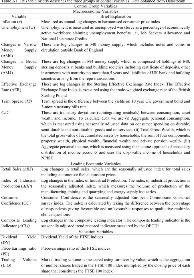
Table A1: This table briefly describes the three groups of control variables. Data obtained from Datastream Control Group Variables
Macroeconomic Variables
Variable Brief Explanation
Inflation (π) Measured as annual log changes in harmonised consumer price index
Unemployment (U) Unemployment is measured as unemployed workforce as a percentage of economically active workforce claiming unemployment benefits i.e., Job Seekers Allowance and National Insurance Credits
Changes in Narrow Money Supply
(ΔM0)
These are log changes in M0 money supply, which includes notes and coins in circulation outside Bank of England
Changes in Broad Money Supply
(ΔM4)
These are log changes in M4 money supply which is composed of holdings of M0, sterling deposits at banks and building societies including certificate of deposits, other instruments with maturity no more than 5 years and liabilities of UK bank and building societies arising from the repo transactions
Effective Exchange
Rate (ΔER)
These are log changes in the Sterling Effective Exchange Rate Index. The Effective Exchange Rate Index is measured using the trade-weighted exchange rate of the British Sterling Pound
Term Spread (TS) Term spread is the difference between the yields on 10 year UK government bond and 3-month treasury bills rate.
CAY These are transitory deviations (cointegrating residuals) between consumption, asset wealth and Income. To calculate CAY we use (i) Aggregate personal consumption, which is measured using seasonally adjusted data on consumer spending on durable, semi-durable and non-durable- goods and on services. (ii) Total Gross Wealth, which is the total gross value of accumulated assets by households; the sum of four components: property wealth, physical wealth, financial wealth and private pension wealth. (iii) Aggregate personal income, which is measured using the income approach of secondary distribution of income accounts and uses the disposable income of households and NPISH
Leading Economic Variables
Retail Sales (ΔRS) Log changes in retail sales, which are the seasonally adjusted index for total sales including automotive fuel at constant prices.
Index of Industrial Production (ΔIIP)
Log changes in the Index of Industrial Production. The index of industrial production is the seasonally adjusted index, which measures the volume of production of the manufacturing, mining and quarrying and energy supply industries
Consumer Confidence (CC)
Consumer Confidence is the seasonally adjusted European Commission consumer survey index. The index is calculated by taking the difference between the percentage of respondents giving favourable and unfavourable responses to qualitative multiple-choice questions.
Composite Leading Indicator (ΔCLI)
Log changes in the composite leading indicator. The composite leading indicator is the seasonally adjusted trend restored indicator measured by the OECD5.
Valuation Variables Dividend Yield
(DY)
Dividend Yield of the FTSE indices Price-Earnings ratio
(PE)
Price-earnings ratio of the FTSE indices Trading Volume
(LIQ)
Market trading volume is measured using turnover by value, which is the aggregation of number shares traded in the FTSE 100 index multiplied by the closing price of each share that constitutes the FTSE 100 index
List of Figures
Figure 1: VFTSE and 360-days implied volatility of FTSE 100 (IVI360) 0 10 20 30 40 50 60 01 /0 2/ 20 00 01 /0 8/ 20 00 01 /0 2/ 20 01 01 /0 8/ 20 01 01 /0 2/ 20 02 01 /0 8/ 20 02 01 /0 2/ 20 03 01 /0 8/ 20 03 01 /0 2/ 20 04 01 /0 8/ 20 04 01 /0 2/ 20 05 01 /0 8/ 20 05 01 /0 2/ 20 06 01 /0 8/ 20 06 01 /0 2/ 20 07 01 /0 8/ 20 07 01 /0 2/ 20 08 01 /0 8/ 20 08 01 /0 2/ 20 09 01 /0 8/ 20 09 01 /0 2/ 20 10 01 /0 8/ 20 10 01 /0 2/ 20 11 01 /0 8/ 20 11 01 /0 2/ 20 12 01 /0 8/ 20 12 01 /0 2/ 20 13 01 /0 8/ 20 13 01 /0 2/ 20 14 01 /0 8/ 20 14 01 /0 2/ 20 15
Implied Volatilites of FTSE 100 index over next 30 and 360 days
VFTSE
List of Tables
Table 1
Descriptive Statistics: Sample.
Panel A
Mean Median Std Dev. Kurt Skew Count
VFTSE (( ) 20.19 18.30 8.00 2.29 1.44 185
IVI360( 360) 21.68 21.06 5.66 0.65 0.79 185
Panel B
Mean (%) Median (%) Std Dev.(%) Kurt Skew Count
FTSE 100 0.89 7.12 14.23 0.89 -0.71 185
FTSE 250 6.75 14.90 17.70 3.57 -1.05 185
Panel C
Mean (%) Median (%) Std Dev. (%) Kurt Skew Count
MKT 1.71 10.00 14.40 1.19 -0.80 185
SMB 3.10 1.29 11.84 2.81 -0.08 185
HML 5.43 3.87 12.07 5.97 -0.03 185
UMD 9.54 13.24 18.93 3.63 -1.08 185
Panel D
Mean Median Std Dev. Kurt Skew Count
Inflation (π) (%) 2.39 2.31 0.95 0.89 0.30 185
Unemployment (U) (%) 3.44 3.10 0.84 -1.26 0.57 185
Narrow Money (ΔM0) (%) 5.46 5.25 1.44 20.60 -2.59 185
Broad Money (ΔM4) (%) 6.18 6.36 3.26 24.09 2.74 185
Effective Exchange Rate (ΔER) (%) -0.69 0.01 5.02 3.92 -0.95 185
Term Spread (TS) (%) 0.99 0.95 1.29 -1.10 0.29 185
CAY 0.004 0.00 0.02 -0.79 0.08 185
Panel E
Mean Median Std Dev. Kurt Skew Count
Retail Sales (∆ )(%) 2.24 2.59 1.05 2.01 -0.38 185
∆ (%) -0.75 0.00 0.95 4.19 -0.99 185
Consumer Confidence -8.16 -5.10 8.96 -0.24 -0.73 185
∆ (%) 0.14 0.16 0.25 2.53 -0.30 185
Panel F
PE ratio Dividend Yield
Mean% Median% Std Dev.% Kurt Skew Mean % Median %Std Dev% Kurt Skew Count
FTSE 100 15.05 14.06 4.51 1.43 1.17 3.32 3.32 0.60 2.06 0.45 185
FTSE 250 18.86 18.76 3.27 1.43 -0.22 2.76 2.63 0.55 4.90 1.92 185
Note: This table reports the descriptive statics. Panel A reports summary statistics of VFTSE (short-term implied market volatility) and IVI360 (long term implied market volatility). Panel B shows the descriptive statistics of annualised excess returns of aggregate FTSE indices. Panel C provides the annualised descriptive statistics of the four popular cross-sectional asset-pricing factors. MKT is the market risk premium; SMB, HML and UMD are size, value and momentum premiums respectively. Panels D, E and F present the descriptive statistics of macroeconomic variables, leading economic indicators and valuation metrics. Sample size: Feb 2000 – June 2015
Table 2
Impact of short and long term implied volatility on the excess returns of FTSE indices Panel A ∆ ∆ ∆ 0 ∆ 4 ∆ Adj.R2 F-stat FTSE 100 -1.72 -0.50*** -0.41* -0.68*** 1.11*** -0.95 -0.15 -0.15 -0.46 20.51 59.87 31.51 (-1.16) (-7.81) (-1.63) (-2.98) (2.83) (-1.24) (-0.95) (-0.81) (-0.85) (1.15) FTSE 250 -2.68* -0.49*** -0.77*** -0.99*** 1.63*** -0.18 -0.25 -0.14 -1.60 34.76*** 58.74 30.11 (-1.79) (-5.69) (-4.30) (-3.00) (3.33) (-0.28) (-1.00) (-0.94) (-1.56) (2.24) Panel B ∆ ∆ Adj.R2 F-stat FTSE 100 -0.44 -0.49*** -0.41** 0.22 0.49** -0.01 2.53*** 61.56% 50.11 (-1.28) (-8.29) (-2.11) (1.39) (2.220 (-0.48) (3.54) FTSE 250 -0.36 -0.49*** -0.72*** 0.24 0.72*** -0.03 4.10*** 61.69% 50.38 (-0.92) (-6.44) (-4.32) (1.00) (2.62) (-1.47) (7.07) Panel C ∆ ∆ Adj.R2 F-stat FTSE 100 6.23*** -0.48*** -0.48*** -1.13* -0.16*** -0.03*** 60.06% 56.33 (2.35) (-11.03) (-2.82) (-1.86) (-2.37) (-3.31) FTSE 250 3.33 -0.51*** -0.69*** -1.85*** 0.12 -0.03* 61.42% 59.57 (1.22) (-6.68) (-4.32) (-3.29) (1.30) (-1.80)
Note: This table reports the results of regression (2a, 2b and 2c). The dependent variables are the monthly excess returns of aggregate FTSE indices. Independent variables are the changes in the 30 days and 360 days implied marketvolatility (∆ ,∆ )after controlling for macroeconomic factors (Panel A), Leading Macroeconomic indicators (Panel B), and valuation factors (Panel C).The figures in parentheses are Newey and West, (1987) heteroscedasticity and autocorrelation corrected t-statistics (pre-whitening with 5 lags) Adjusted sample size March 2000 to July 2015. *** represents significance at 1%, ** at 5% and * at 10%
Table 3
Impact of short and long term implied volatility on the excess returns of FTSE indices
Panel A Panel B
FTSE 100 t-stat FTSE 250 t-stat FTSE 100 t-stat FTSE 250 t-stat 4.25*** (2.09) 4.72 (1.26) 0.04 (0.02) 2.61 (0.78) ∆ -0.48*** (-9.08) -0.49*** (-6.71) -0.56*** (-9.55) -0.59*** (-7.65) ∆ -0.37* (-1.77) -0.61*** (-4.03) -0.30 (-1.45) -0.49*** (-3.10) -1.02*** (-2.77) -2.23*** (-4.20) -0.20 (-0.66) -1.19** (-2.53) -0.21*** (-4.11) 0.01 (0.11) -0.09** (-2.31) -0.003 (-0.03) -0.03*** (-3.89) -0.02 (-1.60) -0.03*** (-3.50) -0.02 (-1.38) 0.03 (0.08) -0.12 (-0.21) 0.14 (0.57) -0.05 (-0.09) 0.68 (1.57) 0.02 (0.03) 0.45 (1.35) -0.07 (-0.10) ∆ 0 -0.51 (-0.77) 0.43 (0.72) -0.52 (-1.25) -0.28 (-0.41) ∆ 4 -0.01 (-0.02) -0.13 (-0.55) 0.04 (0.15) -0.07 (-0.30) ∆ -0.24 (-1.15) -0.32** (-2.13) -0.28 (-1.28) -0.40*** (-2.69) ∆ 0.03 (0.05) -1.04 (-1.10) 0.07 (0.10) -1.16 (-1.19) 11.91 (0.97) 21.01 (1.43) 2.55 (0.25) 7.33 (0.50) ∆ 0.27* (1.95) 0.32 (1.43) 0.28** (2.00) 0.25 (1.08) ∆ 0.29 (1.29) 0.49* (1.86) 0.27 (1.08) 0.53* (1.93) 0.05** (2.22) -0.11** (-2.05) 0.01 (0.31) -0.12** (-2.09) ∆ 3.29*** (2.84) 4.86*** (2.56) 3.00** 2.16 4.91*** (2.62) Adj.R2 34.53% 65.98% 66.73% 65.51% F-statistics 7.10*** 23.31*** 24.19*** 22.96***
Note: This table reports the impact of innovations in the short and the long term implied market volatility on the excess returns of aggregate FTSE indices after controlling for all the variables from the three control group variables together. Panel A uses changes in VFTSE and IVI360 as proxies of innovations in short and long term implied market volatility. Panel B uses the residuals of ARMA (1, 1) models for VFTSE and IVI360 as proxy of innovations in the short and long-term implied market volatility. The t-statistics, reported in parentheses, are corrected for heteroscedasticity and autocorrelation (Newey and West, 1987) pre-whitening with 5 lags. Adjusted sample size, March 2000 to July 2015. *** represents significance at 1%, ** at 5% and * at 10%
Table 4
Factor Loadings on the excess returns of the 25 Size-and-book-to-market portfolios.
Loadings on∆
Small Size 2 Size 3 Size 4 Large Average
Growth 0.33** 0.08 0.06 -0.11 -0.09 0.05 BM2 0.17 0.19 0.09 0.05 -0.14* 0.07 BM3 0.20* 0.16 0.13 -0.05 -0.06 0.08 BM4 0.25* 0.02 0.08 0.02 0.01 0.07 Value 0.17 0.45** 0.23* 0.19 -0.01 0.21 Average 0.22 0.18 0.12 0.02 -0.06 Loadings on changes in∆
Small Size 2 Size 3 Size 4 Large Average
Growth -0.57** -0.1 -0.09 -0.11 0.22** -0.13 BM2 -0.62*** -0.55*** -0.54** -0.34 0.18 -0.37 BM3 -0.78*** -0.55*** -0.76*** -0.38* 0.11 -0.47 BM4 -0.72*** -0.12 -0.27 -0.4 -0.02 -0.31 Value -0.62*** -0.79** -0.54 -0.60** 0.31 -0.45 Average -0.66 -0.42 -0.44 -0.36 0.16 Loadings on MKT
Small Size 2 Size 3 Size 4 Large Average
Growth 1.12*** 1.06*** 1.20*** 0.98*** 0.70*** 1.01 BM2 0.67*** 1.06*** 0.89*** 1.21*** 1.02*** 0.97 BM3 0.77*** 0.81*** 0.88*** 0.87*** 1.08*** 0.88 BM4 0.83*** 0.85*** 1.11*** 0.91*** 0.83*** 0.91 Value 0.84*** 1.28*** 1.10*** 1.26*** 1.11*** 1.12 Average 0.85 1.01 1.04 1.04 0.95 Adjusted R-squared
Small Size 2 Size 3 Size 4 Large Growth 43.81% 39.48% 45.94% 63.40% 57.74% BM2 34.20% 48.30% 57.70% 66.99% 67.78% BM3 47.61% 50.60% 63.33% 69.51% 72.48% BM4 48.20% 44.65% 60.80% 62.08% 70.75% Value 51.95% 51.83% 49.95% 62.90% 50.45% F-statistics
Small Size 2 Size 3 Size 4 Large
Growth 48.56 40.79 52.84 106.67 84.34
BM2 32.7 57.98 84.19 124.78 129.35
BM3 56.44 63.49 106.33 140.09 161.68
BM4 57.77 50.2 95.63 100.85 148.52
Value 66.94 66.62 61.88 104.42 63.12
Note: This table reports the factor loadings from regression (4) for the excess returns of each size-book-to-market portfolio on∆ 30,∆ 360and the market factor (MKT). The associated t-statistics are Newey and West (1987) heteroscedasticity and autocorrelation corrected (pre-whitening with 5 lags). Adjusted sample size March 2000 to July 2015. *** represents
Table 5
Pricing of the innovations in short and long term market implied volatility in the cross-section of the 25
Size-and-Book-to-Market sorted portfolios.
1 2 3 4 0.12 0.60*** 0.13 0.48** (0.55) (3.38) (0.51) (2.49) VFTSE -1.95* -1.73*** -0.97 -1.75*** (-1.95) (-3.81) (-1.07) (-4.78) IVI360 -1.30*** -0.81*** -1.00*** -0.70*** (-3.79) (-5.99) (-3.65) (-6.12) MKT 0.18 -0.22 0.20 -0.08 (0.90) (-1.18) (0.82) (-0.40) SMB 0.16** 0.13*** (2.41) (2.61) HML 0.71*** 0.69*** (6.44) (8.57) UMD -0.43 -0.55 (-0.73) (-1.05)
Note: This table reports the second stage Fama and Macbeth (1973) cross-sectional regressions for the size and book-to-market sorted portfolios. Columns (1) and (2) present the estimates of cross-sectional regressions (5) and (6) respectively. Columns (3) and (4) are the estimates of the same cross-sectional regressions similar, but by using ARMA (1,1) residuals for each of the VFTSE and IVI360 as proxies of innovations in short and long term implied market volatility respectively. MKT, SMB, HML and UMD are market, size, value and momentum factors respectively. The figures in parentheses are heteroscedasticity and autocorrelation corrected t-statistics. *** represents significance at 1%, ** at 5% and * at 10%
Table 6
Factor Risk Premia of the 25 Fama-French portfolios sorted on size and book-to-market characteristics
Factor Risk Premium to∆ (Panel A)
Small Size 2 Size 3 Size 4 Large Average
Growth -0.65 -0.16 -0.12 0.21 0.18 -0.11 BM2 -0.33 -0.38 -0.17 -0.11 0.27 -0.14 BM3 -0.40 -0.31 -0.25 0.10 0.11 -0.15 BM4 -0.49 -0.03 -0.15 -0.04 -0.01 -0.14 Value -0.33 -0.88 -0.45 -0.38 0.03 -0.40 Average -0.44 -0.35 -0.23 -0.04 0.11
Factor Risk Premium to∆ (Panel B)
Small Size 2 Size 3 Size 4 Large Average
Growth 0.74 0.13 0.12 0.14 -0.29 0.17 BM2 0.81 0.72 0.70 0.44 -0.24 0.49 BM3 1.02 0.72 0.99 0.49 -0.14 0.62 BM4 0.94 0.16 0.35 0.52 0.03 0.40 Value 0.80 1.02 0.70 0.78 -0.40 0.58 Average 0.86 0.55 0.57 0.47 -0.21
Factor Risk Premium to MKT (Panel C)
Small Size 2 Size 3 Size 4 Large Average
Growth 0.20 0.19 0.22 0.18 0.13 0.18 BM2 0.12 0.19 0.16 0.22 0.18 0.18 BM3 0.14 0.15 0.16 0.16 0.19 0.16 BM4 0.15 0.15 0.20 0.16 0.15 0.16 Value 0.15 0.23 0.20 0.23 0.20 0.20 Average 0.15 0.18 0.19 0.19 0.17
Note: This table reports the factor risk premia attributable to the changes in short and long term implied volatility. The risk premia are calculated by multiplying the factor loading from table 4 with prices of risk from table 5 column 1.∆ is the changes in the VFTSE Index,∆ is the changes in the IVI360 index, and MKT is the market factor.
Table 7
Pricing of the innovations in short and long term market implied volatility in the cross-section of the 25 Size-and-Book-to-Market sorted portfolios.
1 2 3 4 0.44* 0.17 0.38* 0.13 (1.92) (0.92) (1.68) (0.59) VFTSE -1.80* -2.39** -1.01 -1.76** (-1.78) (-2.42) (-1.60) (-2.08) IVI360 -1.08*** -0.87** -0.93*** -0.78** (-3.35) (-2.37) (-3.27) (-2.12) MKT -0.08 0.26 0.02 0.37 (-0.35) (1.43) (0.08) (1.69) -0.21 -0.11 (-0.93) (-0.50) 0.07 0.16 (0.28) (0.63) ∆ 0 0.14* 0.15** (1.81) (2.14) ∆ 4 0.54** 0.60** (2.16) (2.39) ∆ -0.52 -0.76*** (-1.40) (-2.54) ∆ 0.01 0.01 (0.16) (0.29) CAY -0.01* -0.01** (-1.95) (-2.18) ∆ 0.11 0.25 (0.49) (0.82) ∆ -0.23 -0.22 (-1.14) (-0.75) 4.04*** 5.59*** (3.18) (4.75) ∆ 0.09*** 0.08** (2.72) (2.23)
Note: This table reports the second stage Fama and Macbeth (1973) cross-sectional regressions for the size and book-to-market sorted portfolios. Column 1 presents the estimates of cross-sectional regressions in (7). Column 2 presents prices of risk related to changes in short and long term implied market volatility after controlling for leading economic indicators. Columns 3 and 4 are the estimates of cross-sectional regressions similar to columns 1 and 2, but by using ARMA (1,1) residuals for each of the VFTSE and IVI360 as proxies of innovations in short and long term implied market volatility respectively. Market factor is the market risk premium. The various control factors are explained in Appendix table A1.
CAYis the residuals of the cointegrating equation (3). The figures in parentheses are heteroscedasticity and autocorrelation corrected t-statistics. *** represents significance at 1%, ** at 5% and * at 10%