KRANNERT SCHOOL OF
MANAGEMENT
Purdue University
West Lafayette, Indiana
Cost-Sensitive Decision Tree with Multiple Resource
Constraints
By
Chia-Chi Wu
Yen-Liang Chen
Kwei Tang
Paper No. 1263
Date: January, 2010
Institute for Research in the
Behavioral, Economic, and
Management Sciences
Abstract—Resource constraints are commonly found in classification tasks. For example, there could be a budget limit on
implementation and a deadline for finishing the classification task. Applying the top-down approach for tree induction in this situation may have significant drawbacks. In particular, it is difficult, especially in an early stage of tree induction, to assess an attribute’s contribution to improving the total implementation cost and its impact on attribute selection in later stages because of the deadline constraint. To address this problem, we propose an innovative algorithm, namely, the Cost-Sensitive Associative Tree (CAT) algorithm. Essentially, the algorithm first extracts and retains association classification rules from the training data which satisfy resource constraints, and then uses the rules to construct the final decision tree. The approach has advantages over the traditional top-down approach, first because only feasible classification rules are considered in the tree induction and, second, because their costs and resource use are known. In contrast, in the top-down approach, the information is not available for selecting splitting attributes. The experiment results show that the CAT algorithm significantly outperforms the top-down approach and adapts very well to available resources.
Index Terms—Cost-sensitive learning, mining methods and algorithms, decision trees
I. INTRODUCTION
esource constraints are often imposed on a classification task. In medical diagnosis and marketing campaigns, for example, it is common to have a deadline and budget for finishing the task. The objective
C.-C. Wu is with the Department of Information Management, National Central University, Chung-Li, Taiwan 320, Republic of China. E-mail:
[email protected]. Tel: +886-3-4227151-66569. Fax: +886-3-4254604.
Y.-L. Chen is with the Department of Information Management, National Central University, Chung-Li, Taiwan 320, Republic of China. E-mail:
[email protected]. Tel: +886-3-4267266. Fax: +886-3-4254604.
K. Tang is with the Krannert Graduate School of Management, Purdue University, West Lafayette, IN 47907, USA. E-mail: [email protected]. Tel:
+1-765-494-4464, Fax: +1-765-494-9658
All correspondence should be addressed to Prof. Kwei Tang.
Cost-Sensitive Decision Tree with
Multiple Resource Constraints
Chia-Chi WU, Yen-Liang CHEN, and Kwei TANG
of this paper is to develop an algorithm for tree induction when costs and multiple resource constraints are explicitly considered in developing a decision tree. To our best knowledge, the problem has not been studied in the literature.
Decision trees are one of the most popular predictive models in data mining. The advantages of using a decision tree has been well documented, including its ability to handle high dimensional data, its simple structure in communicating with users, and the fact that its classification results are accurate in many application areas [9]. Many well-known tree induction algorithms have been developed, such as: ID3 [15], C4.5 [16]. CART [3], and GATree [13]. These algorithms are based on a top-down approach, which recursively selects attributes to partition the data to form a hierarchical tree structure with a goal of maximizing classification accuracy or minimizing classification error.
Recently, researchers have discussed economic factors in the process of developing decision trees, such as the costs of procuring, preparing, and storing training datasets and the computational costs of generating classification rules [23]. The research field, known “cost-sensitive decision trees,” explicitly aims to minimizing the total cost of using a tree in classification [20]. Two cost components are often considered: the cost of using attributes in classification, and the cost or penalty incurred by misclassification. For example, in medical diagnosis, attributes may represent the results of diagnosis procedures. If an attribute appears on the decision tree, the cost of performing the diagnosis procedure is incurred for all cases going through the corresponding node [21]. Furthermore, the misclassification cost is the economical consequences associated with classification errors [1]. Studies have concentrated solely
on attribute (test) costs [4][12][18], the misclassification cost [6][7][19][27], or the sum of the two costs [10][11][20][24][26].
Several researchers have considered one resource constraint for a cost-sensitive decision tree. Yang, Ling, Chai, and Pan [24] assumed that patients have a limited budget for performing medical tests and that the tree traveling stops when the limit is reached. Qin, Zhang, and Zhang [14] defined a general problem with one target and one resource component. A top-down algorithm is developed using the ratio of the gain in the target and the resource utilization as the splitting criteria. Chen, Wu, and Tang [4] considered a situation, where multiple targets exist for a classification task. Since targets may share common predictors, it may be beneficial to develop one decision tree with multiple targets, instead of separate trees for individual targets. A top-down approach was used to develop an algorithm for tree induction under a constraint limiting the cost of classifying an instance.
It is well known that the top-down approach is a greedy method, which selects attributes sequentially without back tracking. In other words, the method uses a heuristic attribute selection criterion, and a selected attribute cannot be removed from the tree structure in later stages. Both aspects may result in major drawbacks for using the approach in the situation under consideration. As applied in solving unconstrained problems, it is difficult to assess an attribute’s contribution to improving the goal of the classification task during the tree-induction process. Furthermore, it is especially difficult to evaluate the impact an attribute selected in an early stage on attribute selection in later stages because of the resource constraints. For example, when a medical test is considered in medical diagnosis, the time for performing
the test will limit other tests that can be used when a deadline has been specified for the diagnosis procedure. Note that when one constraint is considered, it is possible to use the cost reduction per unit resource used as a reasonable criterion for selecting a splitting attribute. When multiple constraints are considered, it is difficult to define a reasonable criterion. This further makes the top-down approach even less attractive or effective in this situation.
The drawbacks of the top-down approach motivate the development of an innovative algorithm, as illustrated in Fig. 1. Instead of deriving a decision tree directly from the training dataset, our algorithm consists of two steps. In the first step, we extract association classification rules from the training dataset first and retain those that satisfy the resource constraints. In the second step, we use the association classification rules obtained in the first step to develop a cost-sensitive decision tree.
D R Training Dataset Classification Rules Decision Tree
Fig. 1. The concept of our approach
The algorithm has two main advantages:
(1) Since only feasible classification rules are retained in the first step, we can focus on cost minimization without considering the resource constraints in step 2.
(2) All feasible classification rules are considered in tree induction, whereas the top-down approach considers only those resulting from node splitting.
The remainder of this paper is organized as follows. In Section II, we formalize the problem under consideration, and, in Section III, present the proposed algorithm, namely the Cost-Sensitive Associative Tree (CAT) algorithm. Numerical evaluations of the algorithm are presented in Section IV. A summary and discussion are given in Section V.
II. PROBLEM DEFINITION
A decision tree is built with a training dataset that is usually represented as a relational table shown in Table I. We assume the dataset does not contain missing values. Let A = {A1, A2, …, Am} be the set of all attributes in this table, and C = {c1, c2, …, cn} the set of all classes. Each tuple in the table is a record consisting of attribute values and its corresponding class. We use dk to denote the kth record, ax(dk) the value of Ax of dk, and c(dk) the class of dk.
TABLE I. An Example of Training Data
ID A1 A2 A3 Class 1 A A A T 2 A B B F 3 A A A T 4 B B B T 5 B A A F 6 B A B F 7 C A A F 8 C B B F 9 B A A T 10 A A A T
An item is denoted by (Ax, axi ), where Ax is an attribute andaxi is a possible value of Ax. For
example: (A1, A) is an item. An itemset is a set of items. An itemset is a set of items. {(A1, A), (A3, B)}
is an example of itemset. A record dk can be represented as (att(dk), c(dk)), which is a pair of an itemset and a class, where att(dk) = {(A1, a1(dk)), (A2, a2(dk)), …, (Am, am(dk))}, is the set of all attribute-value pairs of dk. For example, the record with ID 1 can be represented as ({(A1, A), (A2, A), (A3, A)}, T).
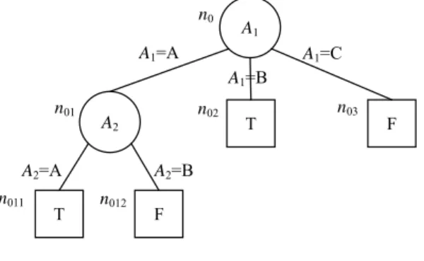
A decision tree TR is a directed acyclic graph. Fig. 2 is an example of a decision tree. We use a circle to represent an internal node and a square to represent a leaf node. We use ni to denote a node in a decision tree, and n0 is the root. An internal node ni in a decision tree is associated with an attribute s(ni) which is used to split ni, while a leaf node nj in a decision tree is labeled with a class l(nj). For example, n0 is an internal node with s(n0) = “A1.” n011 is a leaf node with l(n011) = “T.” <ni, nj> is an edge that links node ni with node nj, where ni is the parent node of nj. v<ni, nj>, which is a possible value of s(ni), the value assigned on edge <ni, nj>. For example, <n0, n01> is an edge that links node n0 with n01, and v< n0, n01> = “A” is the value along this edge, which is a possible value of attribute A1.
F n01 n02 n03 n012 A1=A A1=B A1=C A2=A A2=B A2 T F T n011 A1 n0
Fig. 2. An example of decision tree
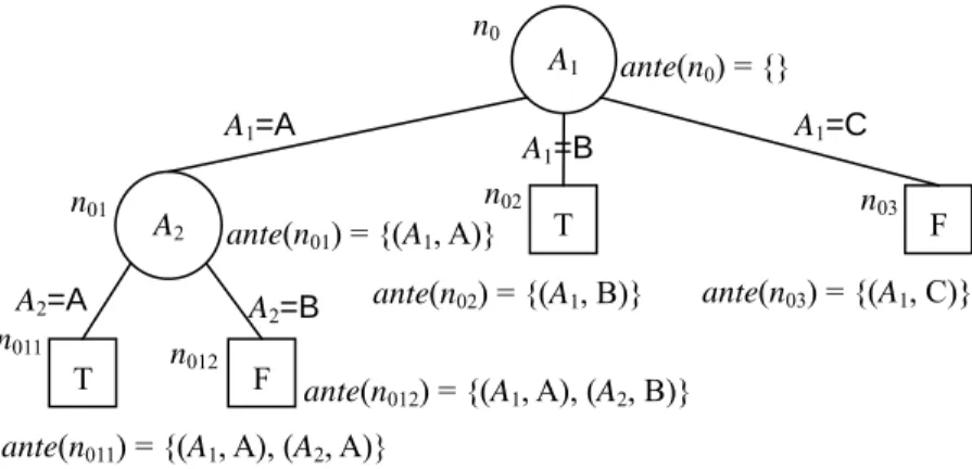
We define ante(ni) as the antecedents of node ni. Suppose the sequence of nodes between the root and ni are n1, n2, n3, …, nm, and the values on edges <n0, n1>, <n1, n2>, …, <nm, ni> are v<n0, n1>, v<n1, n2>, …, v<nm, ni> respectively, ante(ni) = {(s(n0), v<n0, n1>), (s(n1), v<n1, n2>), …, (s(nm), <nm, ni>)}. Fig. 3 shows the antecedents of the nodes in our example decision tree. A record travels the decision tree according to the attributes in the internal nodes and the values on the edges. A record dk can arrive ni if and only if ante
( )
ni ⊆att( )
dk . We useDnito denote a subset of D, where a record dk belongs toi
n
A1 F A2 n0 n01 n02 n03 n012 A1=A A1=B A1=C A2=A A2=B ante(n01) = {(A1, A)} ante(n0) = {} ante(n03) = {(A1, C)}
ante(n011) = {(A1, A), (A2, A)}
ante(n012) = {(A1, A), (A2, B)} T
F T
ante(n02) = {(A1, B)}
Fig. 3. Antecedents of nodes in decision tree
n011
In most of the related studies, a misclassification cost is defined as the cost incurred by assigning a case to class i when it actually belongs to class j. Suppose there are m distinct classes, the misclassification costs can be represented as an m×m matrix. We use MisCost(i, j) to denote the misclassification cost of assigning a case of class j to class i. Consider the example dataset in Table I. There are two classes, “T” and “F”, and the misclassification cost matrix is a 2×2 matrix shown in Table II, where MisCost(T, F) = 10, MisCost(F, T) = 20, and MisCost(T, T) = MisCost(F, F) = 0.
TABLE II.
An Example of Misclassification Cost Matrix
Class T F
T 0 10
F 20 0
When we designate a node as a leaf node and assign a label, the misclassification cost at the node is determined. Let NodeCost(ni) denote the misclassification cost of assigning ni as a leaf node, which is determined using the label that gives the lowest misclassification cost; i.e.,
( )
(
( )
)
⎟⎟ ⎠ ⎞ ⎜ ⎜ ⎝ ⎛ =∑
∈ ∀ ∀ i n k j d D k j l i MisCost l c d n NodeCost min , .corresponding misclassification cost would be 50. In contrast, the cost would be 100 if “F” is assigned. In this case, we have NodeCost(n0) = 50.
Measuring an attribute may consume several types of resources, such as cost and time. We use ResCony(Ax) to denote the number of units of the yth resource needed to measure attribute Ax. For example, the resource consumptions of the attributes in Table I are listed in Table III.
TABLE III.
The Example of Resource Consumptions
Attribute ResCon1(Ax) ResCon2(Ax)
A1 6 5
A2 4 2
A3 2 10
When a record arrives at a node from the root, we must accumulate the number of units of resources consumed to reach the node. We use TotalCony(ni) to denote the total consumption of the yth resource for moving a record from the root node to node ni. Suppose A1, A2, …, and Am are the
attributes appearing in ante(ni), respectively,
( )
∑
( )
= = m x x y i y n ResCon A TotalCon to 1
. For example, in Fig. 1, we have TotalCon1(n02) = 6 and TotalCon2(n011) = 7.
We use MaxResCony to denote the maximum consumption of the yth resource to complete the classification task for a record. For any leaf node ni in a decision tree, the total consumption of any resource TotalCony(ni) cannot exceed MaxResCony.
Given a training dataset, our goal is to develop a cost-sensitive tree that minimizes the total misclassification cost under multiple resource constraints. The proposed algorithm is given in the next section.
III. ALGORITHM
There are three phases in the CAT algorithm:
Phase 1: Extract all classification rules satisfying the resource constraints from the training dataset Phase 2: Build a decision tree from the classification rules extracted in phase 1
Phase 3: Adjust the result of phase 2 to produce the final decision tree
A classification rule r can be represented in form of: condition
( )
r →consequent( )
r . The conditionof this rule is an itemset, and the consequent is a class. For example,
{
(
A1,C) (
, A2,B) (
, A3,A)
}
→T is a classification rule. Semantically, the condition of this rule is a conjunction of items. The rule above can be interpreted as(
A1,C) (
∧ A2,B) (
∧ A3,A)
→T. We use Dr to denote the set of records covered by rule r. That is, a record dk belongs to Dr if and only if condition( )
r ⊆att( )
dk . For example,( )
(A1,A→T)=
{
d1,d2,d3,d10}
=D((A1,A)→F)D . We define cov
( )
r = Dr , the coverage of rule r, which is thenumber of records in D covered by rule r or matching condition(r).
The total consumption of resource y associated with rule r is denoted as RuleCony(r). Suppose A1,
A2, …, and Am are the attributes appearing in condition(r),
( )
∑
( )
= = m x x y y r ResCon A RuleCon to 1 . For example, RuleCon1((A1,C)∧(A2,B) ∧(A3,A)→T) = 12.
We use RuleCost(r) to denote the total misclassification cost of applying rule r to the records in Dr, which is determined by:
( )
∑
(
( ) ( )
)
∈ ∀ = r k D d k d c r consequent MisCost r RuleCost , .matrix in Table II, and the resource consumption matrix shown in Table III. Both thresholds of resource 1 and resource 2 are set to 10.
III.1 Phase 1: Extract classification rules
In this phase, we first extract all classification rules and then prune those rules in rule set Rpruned, where a rule r is in Rpruned if cov(r) is smaller than a threshold mincov or RuleCony(r) > MaxResCony for any resource. We prune rule r∈Rpruned because each rule r corresponds to a node nr in decision tree, where:
• condition(r) = ante(nr)
• consequent(r) = l(nr), suppose that nr is a leaf node • RuleCony(r) = TotalCony(nr) •
( )
r n D r Cov =When cov(r) < mincov, indicating only a small number of records support this rule, the rule is discarded to avoid a potential over-fitting problem. Furthermore, when RuleCony(r) > MaxResCony, the rule is not feasible because the resource constraint associated with the yth resource is violated.
To extract the classification rules, we first transform the relational database D into transaction database DItemset and then find all frequent patterns in DItemset. We use an apriori-like algorithm and find all the frequent itemsets in DItemset which is shown in Table IV. For all records dk belong to D,
( )
dk DItemsetTABLE IV. A DItemset Transformed from Table I.
1 (A1, A), (A2, A), (A3, A) 2 (A1, A), (A2, B), (A3, B) 3 (A1, A), (A2, A), (A3, A) 4 (A1, B), (A2, B), (A3, B) 5 (A1, B), (A2, A), (A3, A) 6 (A1, B), (A2, A), (A3, B) 7 (A1, C), (A2, A), (A3, A) 8 (A1, C), (A2, B), (A3, B) 9 (A1, B), (A2, A), (A3, A) 10 (A1, A), (A2, A), (A3, A)
For each frequent itemset, we select the class that minimizes the misclassification cost as the consequent of the generated rule. For example, consider the frequent itemset (A2, A).
(
)
(
A2,A →T)
=30RuleCost , while RuleCost
(
(
A2,A)
→F)
=80 . Therefore, we generate Rule(
A2,A)
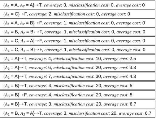
→T from frequent itemset (A2, A).After phase 1, we obtain R, which is the pruned classification rules set extracted from the training dataset. The rules are ranked mainly in terms of the average misclassification cost. Given two rules ri and rj in R, ri precedes rj if •
( )
( )
( )
j( )
j i i r cov r RuleCost r cov r RuleCost < •( )
( )
( )
( )
( )
i( )
j j j i i r cov r cov r cov r RuleCost r cov r RuleCost > ∧ = •( )
( )
( )
( )
( )
i( )
j j j i i r cov r cov r cov r RuleCost r cov r RuleCost = ∧= , but there are less items in the antecedent of ri
than those of rj.
• All the criteria above are tied, but ri was generated earlier than rj.
{A1 = A}→T, coverage: 4, misclassification cost: 10, average cost: 2.5
{A1 = B}→T, coverage: 4, misclassification cost: 20, average cost: 5
{A1 = C}→F, coverage: 2, misclassification cost: 0, average cost: 0
{A2 = A}→T, coverage: 7, misclassification cost: 30, average cost: 4.3
{A2 = B}→T, coverage: 3, misclassification cost: 20, average cost: 6.7
{A3 = A}→T, coverage: 6, misclassification cost: 20, average cost: 3.3
{A3 = B}→F, coverage: 4, misclassification cost: 20, average cost: 5
{A1 = A, A2 = A}→T, coverage: 3, misclassification cost: 0, average cost: 0
{A1 = A, A2 = B}→F, coverage: 1, misclassification cost: 0, average cost: 0
{A1 = B, A2 = A}→T, coverage: 3, misclassification cost: 20, average cost: 6.7
{A1 = B, A2 = B}→T, coverage: 1, misclassification cost: 0, average cost: 0
{A1 = C, A2 = A}→F, coverage: 1, misclassification cost: 0, average cost: 0 {A1 = C, A2 = B}→F, coverage: 1, misclassification cost: 0, average cost: 0
Fig. 4. The extracted rules
III.2 Phase 2: Build a decision tree with extracted rules
In this phase, we build a decision tree from the rules extracted in phase 1. An overview of this phase is shown in Fig. 5.
1. Starting with a single node, root 2. For each non-leaf node, ni
2.1. Make two estimates for each attribute.
2.2. Select the best splitting attribute according to splitting criteria.
2.3. If terminal condition is satisfied, stop splitting and assign ni as a leaf node.
Else, split ni with the splitting attribute of ni.
Fig. 5. An overview of phase 2
Phase 2 starts with a single root marked as n0, the whole training dataset D and R, which is the set
of all the rules extracted in phase 1.
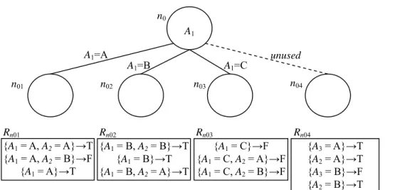
If an attribute Ax was selected to split ni, we use only the rules that contain Ax to classify the records. In other words, rules that exclude Ax have to be discarded. However, since we select the
splitting attribute by estimation, the result may not be globally optimal. Some valuable rules may be discarded because of the estimate error. Therefore, when splitting a node with an attribute Ax, besides the original branches related to each value of Ax, we insert an additional branch marked “unused” to reserve the rules that exclude splitting attribute Ax. Fig. 6 shows the branches and corresponding rule sets after splitting the root with attribute A1.
{A1 = A, A2 = A}→T {A1 = A, A2 = B}→F {A1 = A}→T Rn01 {A3 = A}→T {A2 = A}→T {A3 = B}→F {A2 = B}→T n0 n01 n02 n03 A1=A A1=B A1=C unused n04 {A1 = B, A2 = B}→T {A1 = B}→T {A1 = B, A2 = A}→T Rn02 {A1 = C}→F {A1 = C, A2 = A}→F {A1 = C, A2 = B}→F Rn03 Rn04 A1
Fig. 6. Result of splitting the root node using attribute A1
We use
i
n
EXA to denote the set of attributes that are excluded from ni. For example, EXAn04 =
{ }
A1 .We use
i
n
R to denote a subset of R, where rule rj belongs to Rni if and only if
( )
ni condition( )
rjante ⊆ and any attribute in
i
n
EXA is not in condition(rj). We use Rni
( )
Ax to denote asubset of
i
n
R . A rule rj is in Rni
( )
Ax if rj is in Rni and Ax is in condition(rj). For example, Rn04( )
A3contains two rules: {A3=A}→T and{A3=B}→F.
For each non-leaf node ni, we use two measurements to estimate the effect of using an attribute Ax to split ni. The first is OptCost(ni, Ax), which is the misclassification cost of classifying the records in
i
n
OptCost(ni, Ax) can be regarded as an optimistic estimate of using Ax in ni. The second is PesCost(ni,
Ax), which is the sum of all misclassification costs of the child nodes generated by splitting ni with Ax.
PesCost(ni, Ax) is obtained by supposing that no other attribute will be measured after Ax. Therefore
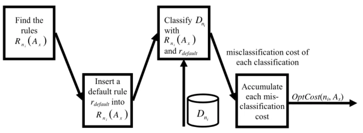
PesCost(ni, Ax) can be regarded as a pessimistic estimate of using Ax in ni. The process of measuring OptCost(ni, Ax) is shown in Fig. 7.
Find the rules Classify with and rdefault Insert a default rule rdefault into Accumulate each mis-classification cost OptCost(ni, Ax) misclassification cost of each classification ( )x n A R i i n D i n D ( )x n A R i Rni( )Ax
Fig. 7. The process of measuring OptCost(ni, Ax)
We first insert a default rule rdefault into the bottom of Rni
( )
Ax , where the condition of rdefault is theantecedent of ni, and the consequent of it is the class that minimizes the misclassification cost. Then, we classify the records in
i
n
D with the rules in Rni
( )
Ax and the default rule. For a record dk in Dni, thefirst rule that covers the attribute values of dk classifies it. The classification result may cause a misclassification cost. The accumulation of all the misclassification costs is the value of OptCost(ni, Ax).
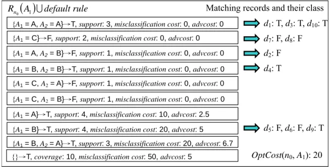
An example is shown in Fig. 8. For measuring OptCost(n0, A1), we use the rules in Rn0with A1 in
their conditions and the default rule, {}→T, to classify the records belonging toDn0. The value of
OptCost(n0, A1) = 20.
( )
A default rule Rn0 1 ∪{A1 = A}→T, support: 4, misclassification cost: 10, advcost: 2.5
{A1 = B}→T, support: 4, misclassification cost: 20, advcost: 5
{A1 = C}→F, support: 2, misclassification cost: 0, advcost: 0
{A1 = A, A2 = A}→T, support: 3, misclassification cost: 0, advcost: 0
{A1 = A, A2 = B}→F, support: 1, misclassification cost: 0, advcost: 0
{A1 = B, A2 = A}→T, support: 3, misclassification cost: 20, advcost: 6.7
{A1 = B, A2 = B}→T, support: 1, misclassification cost: 0, advcost: 0
{A1 = C, A2 = A}→F, support: 1, misclassification cost: 0, advcost: 0 {A1 = C, A2 = B}→F, support: 1, misclassification cost: 0, advcost: 0
{}→T, coverage: 10, misclassification cost: 50, advcost: 5
d1: T, d3: T, d10: T d7: F, d8: F d2: F d4: T d5: F, d6: F, d9: T OptCost(n0, A1): 20
Matching records and their class
Fig. 8. The example of measuring OptCost(n0, A1)
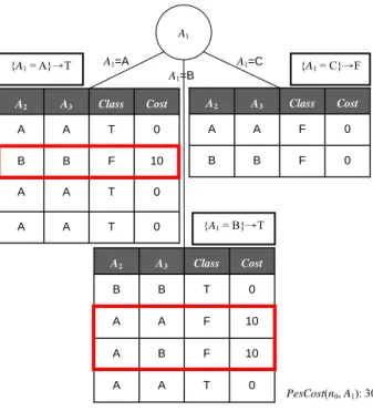
The value of PesCost(ni, Ax) is estimated by assuming that after splitting ni with Ax all the immediate children will be leaf nodes. Suppose that the label of each leaf node is determined by the class with the minimal misclassification cost. Then, the value of PesCost(ni, Ax) will be equal to the sum of all misclassification costs of the child nodes generated by splitting ni with Ax. However, if a node has too few data or no data, we use the minimal misclassification cost label of its parent as its label.
Consider the example shown in Fig. 9, where three child nodes are generated by splitting n0 with
A1. If no other attributes will be measured after A1, there are only three rules:
{
A1 =A}
→T ,{
A1 =B}
→T , and{
A1 =C}
→Fthat can be used to classify the records in Dn0 . The value ofPesCost(n0, A1) is the accumulation of all misclassification costs of the classifications, and the result is
0 0 10 0 Cost A A B A A3 T T F T Class A A B A A2 0 10 10 0 Cost A B A B A3 T F F T Class A A A B A2 0 0 Cost B A A3 F F Class B A A2 A1 A1=A A1=B A1=C PesCost(n0, A1): 30 {A1 = C}→F {A1 = B}→T {A1 = A}→T
Fig. 9. The example of measuring PesCost(n0, A1)
For each non-leaf node ni, if there exists any attribute Ax where OptCost(ni, Ax) < NodeCost(ni), select an attribute Ay which has the minimum OptCost(ni, Ay) to further split node ni. If there is more than one attribute having the minimum OptCost, from them we select the attribute with the minimum PesCost. If OptCost(ni, Ax)≥NodeCost(ni) for all attributes Ax, assign ni as a leaf, and label ni with the class that minimizes NodeCost(ni). In our example, both OptCost(n0, A1) and OptCost(n0, A2) are 20, but PesCost(n0, A1) = 30, which is smaller than PesCost(n0, A2) = 50. Therefore, A1 is selected to be the
splitting attribute of the node n0.
Suppose attribute Ax has m possible values. When ni is split by Ax, there will be (m+1) child nodes emanated from ni, where m of them correspond to the values of Ax and the last one is connected to ni by an edge marked “unused.” For the last node nu, which is connected with the “unused” edge, ante(nu) = ante(ni), EXAnu = EXAni ∪
{ }
Ax . For any other nodes nj, ante( )
nj =ante( )
ni ∪{
(
Ax,v(
ni,nj)
)
}
, andi
j n
n EXA
EXA = . In our example, there are three possible values of A1. After splitting n0 with A1, there
are four child nodes produced from n0, as shown in Fig. 6. Among the four child nodes, ante(n01) =
{(A1, A)}, and EXAn01 = {}, while ante(n04) = {}, and EXAn04 = {A1}.
Let nh be the parent of ni. A node ni will stop splitting and become a leaf node if and only if: • No attribute is selected by the splitting criterion.
• There exists only one rule r in , i
n
R where condition(r) = ante(ni). This may be caused by the fact that further splits at ni will result in violation of at least one resource constraint, or by the fact that there are not sufficent records in all branches of ni. In this case, we stop splitting at ni and label ni with the consequent of r.
• There exists no rule in .
i
n
R This condition occurs because the number of records in some child nodes of nh exceeds mincov, but in ni it does not. In this case, ni will be labeled with the class that minimizes the misclassification cost of nh.
• There exist multiple rules in ,
i
n
R and OptCost(nh, s(nh)) = PesCost(nh, s(nh)). The equality of
OptCost(nh, s(nh)) and PesCost(nh, s(nh)) indicates that the misclassification cost cannot be reduced after splitting nh, the parent node of ni. Therefore, we should stop splitting at ni and label it with the class that minimizes the misclassification cost of ni.
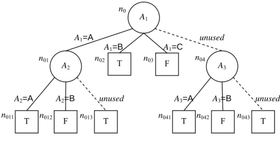
n011 A1 n0 n01 n02 n03 A1=A A1=B A1=C unused n04 A2=A A2=B unused T A3=A A3=B unused n012 n013 n041 n042 n043 A2 F A3 T F T T F T
Fig. 10. The output of phase 2
III.3 Phase 3: Adjustment for producing the final decision tree
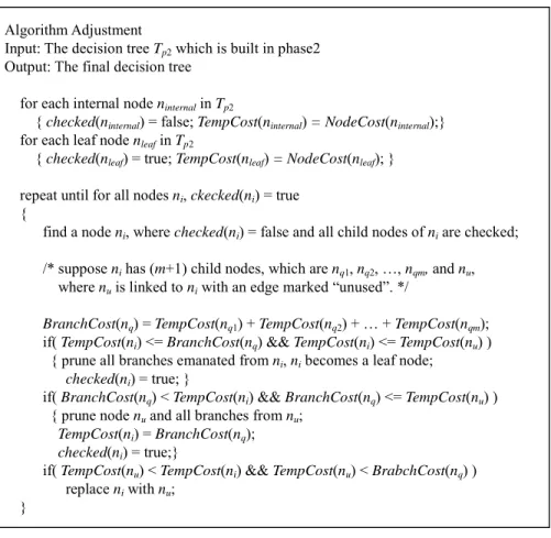
In phase 2, we build a tree from the classification rules extracted in phase 1. During the tree- induction process, we iteratively generate new branches from internal nodes. Although two measurements have been used to help evaluate whether an internal node should be further split or just stopped as a leaf node, it is difficult to make an accurate evaluation unless we have the final complete tree. Therefore, in phase 3, we will re-examine the entire tree carefully from bottom to top to determine whether there are any unnecessary branches. In other words, we hope to improve the tree by pruning unnecessary branches or nodes. The detailed procedure of phase 3 is shown in Fig. 11.
Algorithm Adjustment
Input: The decision tree Tp2 which is built in phase2
Output: The final decision tree for each internal node ninternal in Tp2
{ checked(ninternal) = false; TempCost(ninternal) = NodeCost(ninternal);}
for each leaf node nleaf in Tp2
{ checked(nleaf) = true; TempCost(nleaf) = NodeCost(nleaf); }
repeat until for all nodes ni, ckecked(ni) = true
{
find a node ni, where checked(ni) = false and all child nodes of ni are checked;
/* suppose ni has (m+1) child nodes, which are nq1, nq2, …, nqm, and nu,
where nu is linked to ni with an edge marked “unused”. */
BranchCost(nq) = TempCost(nq1) + TempCost(nq2) + … + TempCost(nqm);
if( TempCost(ni) <= BranchCost(nq) && TempCost(ni) <= TempCost(nu) )
{ prune all branches emanated from ni, ni becomes a leaf node;
checked(ni) = true; }
if( BranchCost(nq) < TempCost(ni) && BranchCost(nq) <= TempCost(nu) )
{ prune node nu and all branches from nu;
TempCost(ni) = BranchCost(nq);
checked(ni) = true;}
if( TempCost(nu) < TempCost(ni) && TempCost(nu) < BrabchCost(nq) )
replace ni with nu;
}
Fig. 11. The algorithm of phase 3
For each node ni in the decision tree generated in phase 2, we use checked(ni) to indicate whether ni is checked. For a checked node ni, TempCost(ni) is used to store the misclassification cost of the subtree with the root node ni. Initially, for all nodes ni, TempCost(ni) is set to be NodeCost(ni) and is updated as we produce the final tree. Furthermore, checked(ni) is set to be “false” for all internal nodes, and checked(ni) “true” for all leaf nodes.
We adjust the tree from the bottom to the top by repeatedly processing all unchecked nodes, whose child nodes have been checked. Consider a node ni as shown in Fig. 12. Suppose there are (m+1) child nodes of ni, where nq1, nq2, …, and nqm correspond to the values of s(ni), and nu is linked to ni with an edge marked “unused.” Additionally, all the (m+1) child nodes of ni are checked.
BranchCost(nq) = TempCost(nq1) + … + TempCost(nqm) ni unused ……. nq1 nq2 nqm nu Child of nu Child of nu BranchCost(nu)= TempCost(nu)
Fig. 12. A node being processed in phase 3 NodeCost(ni) = TempCost(ni)
We compare three costs:
• NodeCost(ni): the misclassification cost of assigning ni as a leaf node, which is equal to TempCost(ni).
• BranchCost(nq): the total misclassification cost of classifying the data in Dniusing the subtrees
with the root nodes: nq1, nq2, …, and nqm. The value of BranchCost(nq) is obtained by summing TempCost(nq1), TempCost(nq2), …, and TempCost(nqm).
• BranchCost(nu), the misclassification cost resulting from classifying the data in Dniusing the
subtree with the root node nu. That is, attribute s(ni) will not be used. Instead, classification will be performed using s(nu).
There are three cases about the comparison result. These three cases correspond to the following three situations:
Case 1: NodeCost(ni)≤BranchCost(nq) and NodeCost(ni)≤BranchCost(nu). In this case, further splitting cannot reduce the misclassification cost of the records in node ni. Therefore, we prune all
branches generated from ni, and ni becomes a leaf node.
Case 2: BranchCost(nq)<NodeCost(ni) and BranchCost(nq)≤BranchCost(nu). In this case, it is beneficial to use s(ni) to classify the data in Dni. Therefore, we prune nu and its sub-branches.
Case 3: BranchCost(nu)<BranchCost(nq) and BranchCost(nu)<NodeCost(ni). In this case, it is not beneficial to use s(ni) to classify the data in Dni. Therefore, we replace ni with nu.
Fig. 13 displays the adjustments in the three cases. For example, consider the node n01 in the figure
10, whose splitting attribute is A2. There are three child nodes of n01. Two of them are n011 and n012,
which related to “A2=A” and “A2=B,” respectively, and the last child node n013 is linked to n01 with an
edge marked “unused.” After computation, we have NodeCost(n01) = 10, NodeCost(n011) +
NodeCost(n012) = 0, and NodeCost(n013) = 10. Obviously, NodeCost(n011) + NodeCost(n012) is the
smallest one. Therefore, we prune n013.
In Cases 1 and 2, checked(ni) will be set to be true. We only need to update TempCost(ni) in Case 2 by setting it equal to BranchCost(nq). In our example, the values of TempCost(n01) and checked(n01) become “0” and “true,” respectively. After this phase, the final tree of our example is shown in Fig. 2. Note that , in Case 3, since the sub-tree with the root node ni is replaced by that with the root node nu, it is not necessary to update TempCost(ni).
ni … nq1 nq2 nqm nu ni Case 1 ni nq1 nq2 … nqm Case 2 nu Case 3
Fig. 13. Adjustments of three cases
IV. PERFORMANCE EVALUATION
In this section, we perform experiments to evaluate the proposed algorithm, CAT. Twelve datasets obtained from the UCI Machine Learning repository [2][5] are used in the experiments. A description of these datasets is given in Table V. The numerical attributes in the datasets are discretized using the minimal entropy method in the data preparation stage [8]. Furthermore, we removed all records containing missing values
TABLE V. Datasets We Adapted in Experiments
Dataset Number of attributes
Number of
examples Class distribution
Acute
Inflammations(D1) 6 120 no: 61 yes: 59
Acute
Inflammations(D2) 6 120 no:70 yes: 50
Car 6 1728 unacc: 1210 good: 69 acc: 384 v-good: 65 Contraceptive Method Choice 9 1473 1: 629 3: 511 2: 333 Credit Approval 15 690 +: 307 -: 383 Heart Disease 13 303 0: 164 1: 139 Nursery 8 12960 not_recom: 4320 very_recom: 328 spec_prior: 4044 recommend: 2 priority: 4266 Pima Indians
Diabetes 8 768 Healthy: 500 Diabetes: 268 Thyroid Disease 20 3772 Hypothroid: 93 Hyperthyroid: 191
Normal: 3488
Tic-Tac-Toe 9 958 positive:626 Negative:332
Voting 16 435 Democrat: 267 Republican: 168
Zoo 16 101 1: 41 5: 4 2: 20 6: 8 3: 5 7: 10 4: 1
We compare the CAT algorithm, labeled as M4, with four additional approaches, M0 through M3 described in Table VI, in the experiments. Note that M0 is used as a baseline, which represents an approach without using a classification model.
TABLE VI. Five Methods in the Experiment
Methods Description M0 Classify an instance to the class, which minimizes the misclassification cost. M1 A top-down approach, which selects the splitting attribute with the maximum
reduction in the misclassification cost. Resource constraints are not considered. M2 A top-down approach, which selects the splitting attribute with the smallest sum of
the total misclassification cost and the total resource usage.
M3 A top-down approach, which selects the splitting attribute with the largest ratio of the reduction in the total misclassification cost and the total resource usage. M4 CAT
Most of the original datasets do not contain cost information. For our experiments, the misclassification costs are determined by the distribution of the class labels. Following the method in [11] and [26], we use 200 as the baseline for the per-case cost of misclassification and make adjustments so that the cost is higher for misclassifying rare classes. For example, in the Pima Indians Diabetes dataset, the ratio of the Healthy label to the Diabetes level is roughly 2 to 1. Therefore, we set the costs of misclassification for this dataset as MisCost (1, 0) = 200 and MisCost (0, 1) = 400.
We ran a cross validation in each experiment. Datasets were randomly split into ten parts. Ten pairs of the training and test datasets were generated, where the test dataset involved one partition and the training dataset involved the other nine partitions. We built decision trees with the training datasets and evaluate the trees with the test datasets. The final result from each experiment is the average of the results obtained with the ten pairs of training and test datasets.
resource constraint (Section IV.1), two resource constraints (Section IV.2), and multiple resource constraints (Section IV.3).
IV.1 Performance evaluation under a single constrained resource
We first evaluate the four methods under one resource constraint. In order to determine a possible upper bound on MaxResCon for a dataset, we first obtain a decision tree by M1 without any resource constraints and obtain the maximal resource consumption, denoted by MaxTotalCon, to arrive a leaf node. To observe how the scarcity of resource impacts performance, we obtain the results by gradually reducing MaxResCon from MaxTotalCon to 90%×MaxTotalCon, 80%×MaxTotalCon, …, and 20%×MaxTotalCon. Furthermore, we randomly set the resource consumption of each attribute between 1 and 100, and the minimal coverage threshold mincov 5%.
The results are presented in Table VII, where the columns list the levels of available resources, the rows show the datasets and the four approaches, and the cell show values that are the ratio of the misclassification cost of the corresponding approach and resource level to that of M0. The results are analyzed by a three-factor ANOVA model, where the three-way interaction is not used, because no replications were performed under each treatment level. It was found that the three main effects, Dataset, Method, and Percentage, are statistically significant at the 5% level, and the two-way interactions are also significant, except that between Dataset and Method. The results of Tukey’s multiple comparisons indicate that CAT significantly outperforms the other three approaches, and that M2 is significantly better than M1 and M3. These results are expected because our method benefits
from selecting splitting attributes according to all possible sequences of attributes, whereas the traditional top-down approach considers only the result of splitting a present node.
TABLE VII.
EXPERIMENT RESULTS FOR EACH METHOD IN DIFFERENT DATASETS
Dataset Method MaxResCon (form 100%×MaxTotalCon to 20%×MaxTotalCon) 100% 90% 80% 70% 60% 50% 40% 30% 20% Acute Inflammations (D1) M1 0.1475 0.1639 0.1639 0.1639 0.1639 0.1639 0.1639 0.3443 0.4098 M2 0.1639 0.1639 0.1639 0.1639 0.1639 0.1639 0.1639 0.3279 0.3279 M3 0.1639 0.1639 0.1639 0.1639 0.1639 0.1639 0.1639 0.1639 0.3279 M4 0.0000 0.0000 0.0000 0.0000 0.0000 0.1639 0.1639 0.1639 0.3279 Acute Inflammations (D2) M1 0.0000 0.1429 0.1429 0.1429 0.1429 0.1429 1.0000 1.0000 1.0000 M2 0.0000 0.1429 0.1429 0.1429 0.1429 0.1429 0.4200 0.7714 0.7714 M3 0.0000 0.1429 0.1429 0.1429 0.1429 0.1429 0.7543 0.7714 0.7714 M4 0.0000 0.0000 0.0000 0.0000 0.1429 0.1429 0.4200 0.7714 0.7714 Car M1 0.4999 0.4999 0.4999 0.5768 0.5768 0.5768 0.5768 0.6656 0.6752 M2 0.5321 0.5321 0.5321 0.5321 0.5321 0.5321 0.5321 0.5068 0.6752 M3 0.6816 0.6816 0.6816 0.6816 0.6816 0.6816 0.6816 0.6816 0.8015 M4 0.4999 0.4999 0.4999 0.5280 0.5280 0.5086 0.5086 0.5068 0.6752 Contraceptive Method Choice M1 0.8394 0.8394 0.8394 0.8394 0.8340 0.8340 0.8517 0.8606 0.8695 M2 0.8780 0.8780 0.8780 0.8780 0.8780 0.8780 0.8869 0.8869 0.8737 M3 0.8699 0.8699 0.8699 0.8699 0.8699 0.8699 0.8737 0.8737 0.8737 M4 0.7506 0.7641 0.7618 0.7552 0.7548 0.7263 0.7811 0.8039 0.8069 Credit Approval M1 0.2600 0.2600 0.2600 0.2600 0.2600 1.0000 1.0000 1.0000 1.0000 M2 0.4790 0.4790 0.5995 0.5995 0.6081 0.6342 0.6342 0.6752 0.6752 M3 0.4005 0.4005 0.4005 0.4005 0.5916 0.7133 0.6860 0.7099 0.7099 M4 0.2895 0.2782 0.2691 0.2600 0.2600 0.5540 0.5614 0.6752 0.6752 Heart Disease M1 0.5500 0.5500 0.5500 0.5500 0.5500 0.5500 0.5500 0.6090 0.6090 M2 0.4718 0.4718 0.4718 0.4718 0.4718 0.4718 0.4718 0.4718 0.5090 M3 0.4885 0.4885 0.4885 0.4885 0.4885 0.4885 0.4885 0.4885 0.5090 M4 0.4910 0.4231 0.3615 0.3782 0.4474 0.4359 0.4641 0.4295 0.4872 Nursery M1 0.2970 0.2970 0.2970 0.2970 0.2970 0.4686 0.4686 1.0000 1.0000 M2 0.3248 0.3248 0.3248 0.3248 0.3248 0.3979 0.4247 0.7671 0.8290 M3 0.6982 0.6982 0.6982 0.6982 0.6982 0.6982 0.6982 0.7671 0.8290 M4 0.2970 0.2970 0.2970 0.2970 0.2970 0.3932 0.4247 0.6982 0.7860 Pima Indians Diabetes M1 0.5720 0.5720 0.5720 0.5640 0.5460 0.5460 0.5460 0.5760 0.5760 M2 0.5580 0.5580 0.5580 0.5380 0.5380 0.5500 0.5460 0.5860 0.6060 M3 0.5660 0.5660 0.5660 0.5460 0.5460 0.5460 0.5460 0.5860 0.6060 M4 0.5480 0.5480 0.5800 0.5620 0.5140 0.5640 0.5440 0.5300 0.5760 Thyroid Disease M1 0.5078 1.0000 1.0000 1.0000 1.0000 1.0000 1.0000 1.0000 1.0000 M2 0.5078 0.6765 0.6765 0.6765 0.6765 0.6765 0.6765 0.9802 0.9903 M3 0.8118 0.8118 0.8141 0.8118 0.8118 0.8118 0.8118 0.9802 0.9903 M4 0.5078 0.6241 0.6241 0.6765 0.6765 0.6765 0.6765 0.9994 0.9877 Tic-Tac-Toe M1 0.6725 0.6725 0.6725 0.6725 0.6565 0.6565 0.6677 1.0000 1.0000 M2 0.8035 0.8035 0.8035 0.8035 0.8035 0.8035 0.8035 0.8083 0.8083 M3 0.6645 0.6645 0.6645 0.6645 0.6645 0.6837 0.7013 0.7971 0.8115 M4 0.5304 0.5112 0.5687 0.6358 0.6166 0.6374 0.6629 0.7812 0.7875 Voting M1 0.0585 1.0000 1.0000 1.0000 1.0000 1.0000 1.0000 1.0000 1.0000 M2 0.2621 0.2621 0.2621 0.2621 0.2903 0.2903 0.2903 0.2903 0.2903 M3 0.3891 0.3427 0.3569 0.3367 0.3992 0.3992 0.3931 0.3972 0.3629 M4 0.0585 0.2540 0.3044 0.3024 0.3327 0.2722 0.2621 0.2903 0.2903 Zoo M1 0.2283 0.2283 0.2283 0.2283 0.2862 0.4239 0.4239 0.4239 1.0000 M2 0.3297 0.3297 0.3297 0.3297 0.3297 0.3297 0.3297 0.4239 0.1957 M3 0.1848 0.1848 0.1848 0.1848 0.1848 0.1848 0.1848 0.1848 0.2065 M4 0.0725 0.0725 0.1558 0.1558 0.1413 0.1667 0.1522 0.1920 0.1993
IV.2 Performance evaluation under two resource constraints
the attribute costs, and the other for the completion time. The Heart Disease dataset is used in the evaluation. The dataset was made available by Robert Detrano of the Cleveland Clinic Foundation. The attribute costs and times given in Table VIII are obtained from the literature [17][20]. In addition, the misclassification costs are MisCost(1, 0) = 600 and MisCost(0, 1) = 1,000 [17].
TABLE VIII.
THE ATTRIBUTES IN THE HEART DISEASE DATASET Attribute/Test Test Fee (CN$) Test Time (Minutes) Description
num - - diagnosis of a heart disease
0: less than 50% artery narrowing; 1: more than 50% artery narrowing
age 1.00 1 in years
sex 1.00 1 sex (1 = male; 0 = female)
cp 1.00 1 chest pain type
1: typical angina; 2: atypical angina; 3: non-anginal pain; 4: asymptomatic
trestbps 1.00 1 resting blood pressure (in mm Hg on admission to the hospital) chol 7.27 240 serum cholestoral in mg/dl
fbs 5.20 240 fasting blood sugar > 120 mg/dl restecg 15.50 30 resting electrocardiographic results thalach 102.90 60 maximum heart rate
exang 87.30 60 exercise induced angina (1 = yes; 0 = no) oldpeak 87.30 60 ST depression induced by exercise relative to rest
slope 87.30 60 the slope of the peak exercise ST segment ca 100.90 60 number of major vessels (0-3) colored by flourosopy thal 102.90 60 3 = normal; 6 = fixed defect;
7 = reversible defect
As in Section IV.1, the four methods are compared under different limits for the two constraints. We first obtain the decision tree for M1 and evaluate the resource use, MaxTotalCon1 and
MaxTotalCon2, respectively, for time and cost. Three levels – 75%, 50%, and 25% of MaxTotalCon1 –
are used for the time constraint, whereas the limit for the cost constraint remains at MaxTotalCon2.
Fig. 14. The ratio of misclassification cost of each method for datasets Heart Disease under
(a)MaxResCon1 = 75%×MaxTotalCon1, (b) MaxResCon1 = 50%×MaxTotalCon1, and (c)MaxResCon1 = 25%×MaxTotalCon1
From the results shown in Fig.14, the proposed method, CAT, is clearly the overall best performer, especially under tight resource constraints. This finding empirically demonstrates that CAT is very effective in reducing the misclassification cost under limited resources. Furthermore, the performance of M2 and M3 are generally not affected by resource constraints. These results suggest that a top-down approach is unable to adapt to the availability of resources, especially when resources are abundant.
IV.3 Performance evaluation under multiple resource constraints
We use all the datasets listed in Table V in this section. Since the cost and time information for most of these datasets are not available, we generate the values randomly in our evaluation. Five resource constraints are considered with the consumption rate of each resource by each attribute was set randomly between 1 and 100. For each constrained resource Resy, the resource constraint
25%×MaxTotalCony.
The results are shown in Table IX, where the columns represent the number of constrained resources, the rows give the various alternatives, and the cell values show the ratio of the misclassification cost resulting from this method and the misclassification cost resulting from M0.
TABLE IX
EXPERIMENT RESULTS OF DIFFERENT NUMBER OF CONSTRAINED RESOURCE
DataSet Method Number of Constrained Resource DataSet Method Number of Constrained Resource
1 2 3 4 5 1 2 3 4 5 Acute Inflammations (D1) M1 0.1639 0.1639 0.1639 1.0000 1.0000 Nursery M1 0.4686 0.4686 1.0000 1.0000 1.0000 M2 0.1639 0.1639 0.1639 0.8361 0.8361 M2 0.4797 0.7689 0.8404 0.8404 0.8404 M3 0.1639 0.1639 0.1639 0.4754 0.8361 M3 0.5102 0.6932 0.8404 0.8404 0.7860 M4 0.0000 0.1639 0.1639 0.4754 0.8197 M4 0.3633 0.4686 0.7860 0.7860 0.7860 Acute Inflammations (D2) M1 0.2000 1.0000 1.0000 1.0000 1.0000 Pima Indians Diabetes M1 0.5720 0.5900 0.5900 0.5900 0.5900 M2 0.2000 0.8000 0.8000 1.0000 1.0000 M2 0.5340 0.6900 0.7300 0.6900 0.8120 M3 0.0000 0.8000 0.4000 1.0000 1.0000 M3 0.5340 0.6900 0.7280 0.5900 0.5900 M4 0.0000 0.4200 0.4000 1.0000 1.0000 M4 0.5280 0.5900 0.5900 0.5900 0.5900 Car M1 0.5983 0.6752 0.6752 0.6752 0.6752 Thyroid Disease M1 1.0000 1.0000 1.0000 1.0000 1.0000 M2 0.5321 0.7013 0.7460 0.7820 0.7820 M2 0.6937 0.8769 0.6937 1.0000 1.0000 M3 0.5399 0.7013 0.6752 0.7820 0.6752 M3 0.8769 0.8769 0.6937 1.0000 1.0000 M4 0.5327 0.7074 0.6752 0.6752 0.6752 M4 0.6937 0.6937 0.6937 1.0000 1.0000 Contraceptive Method Choice M1 0.8429 0.8429 0.8695 0.8695 0.8695 Tic-Tac-Toe M1 0.6725 0.6725 0.6725 0.6805 0.6805 M2 0.8672 0.8610 0.8707 0.9004 0.8695 M2 0.6581 0.6693 0.6326 0.8227 0.6486 M3 0.8683 0.8544 0.8436 0.8695 0.8695 M3 0.6757 0.6677 0.6470 0.6486 0.6597 M4 0.7483 0.7471 0.7737 0.7795 0.8695 M4 0.6022 0.5879 0.6278 0.6645 0.6294 Credit Approval M1 0.2600 0.2600 1.0000 1.0000 1.0000 Voting M1 1.0000 1.0000 1.0000 1.0000 1.0000 M2 0.3430 0.5529 0.7799 0.7799 0.5563 M2 0.2742 0.3548 0.3065 0.3065 1.0000 M3 0.2600 0.2600 0.7309 0.5563 0.5563 M3 0.3548 0.3548 0.3065 0.3065 1.0000 M4 0.2691 0.2600 0.5563 0.5563 0.5563 M4 0.2601 0.2984 0.3065 0.3065 1.0000 Heart Disease M1 0.5500 0.5500 0.5449 0.5449 0.5974 Zoo M1 0.2283 0.2283 0.2283 0.2283 0.4239 M2 0.5346 0.6038 0.5590 0.5603 0.6538 M2 0.2935 0.2935 0.2862 0.2862 0.3188 M3 0.5372 0.4577 0.5321 0.5551 0.6218 M3 0.2971 0.2935 0.2862 0.2862 0.3188 M4 0.4577 0.4551 0.4551 0.4744 0.4962 M4 0.0870 0.1594 0.2174 0.1159 0.2609
As shown in Table IX, in a majority of the cases, as the number of constrained resources increases, the number of attributes that can be used decreases and the misclassification cost increases. In some cases, the performances of the four methods are roughly the same. This phenomenon happens when the depth of the tree is short because only a small number of attributes can be used as the resource constraints become tight. As a result, the variation in selected attributes is small among the four methods. However, CAT, still achieved a better or at least comparable performance, compared with the other three methods. The results from the statistical analysis using a three-factor ANOVA model show
CAT significantly outperforms the other three methods in the average cost. However, M2 and M3 are not significantly different in their performances.
From the results of the experiment presented in this section, we conclude that the proposed algorithm, CAT, outperforms the top-down approach and produces satisfactory results in all the situations under consideration.
In order to study the time complexity of CAT, we use the Nursery dataset, which has 12,960 records and 8 attributes, to show the effect of the number of records on its computation time. We also use the Zoo dataset, which has 16 attributes and 101 records, to show the effect of the number of attributes. The results are reported in Figure 15, where the total computation time is plotted against the number of attributes or records.
Fig. 15. The computation time of (a) different data size of Nursery dataset (b) different number of attribute of zoo dataset Time (second)
No. of Records (1,000)
Time (second)
No. of Attributes
(a) (b)
The figure shows the total computation time increases linearly as the number of attributes or records increases, suggesting the proposed method performs satisfactorily. It is evident that phase 1 consumes a large portion of the computation time. Note that, in phase 1, the Apriori algorithm is modified to generate association rules, which satisfy the mincov threshold. We follow the same
approach to develop an Apriori-like approach to work simultaneously for resource constraints. This combination effectively reduces the computation time by systematically pruning un-desired rules with respect to mincov and resources in early stages. The results suggest this approach works efficiently.
V. CONCLUSION AND FUTURE STUDIES
Cost-sensitive classification has been a popular research topic in recent years. In this paper, we study a problem of developing a cost-sensitive decision tree under multiple resource constraints. A new algorithm is developed to address the drawbacks of the traditional top-down approach to tree induction. The algorithm consists of two steps. In the first step, we extract association classification rules from the training dataset first and retain those that satisfy the resource constraints. In the second step, we use the association classification rules obtained in the first step to develop a cost-sensitive decision tree. Because only feasible classification rules are extracted and retained in step 1, it is not necessary to consider resource constraints in step 2. The results of an extensive numerical experiment show that the proposed algorithm produces satisfactory results under different tightness levels of resource constraints and outperforms the top-down approach.
There are several possible extensions to this study. First, we allow only attributes as predictors in the proposed algorithm. An implicit assumption is that we would have to perform discretization to allow using numerical variables in the algorithm. An extension allowing direct use of numerical variables would broaden the applicability of the algorithm. Furthermore, we assume no missing values
in developing the proposed algorithm. The internal node strategy, proposed by Ling, et.al [10] and adopted by Zhang, et al. [26], may be incorporated in the proposed algorithm to handle missing data.
Zadrozny, Langford, and Abe [25] developed a novel method for generating cost-sensitive trees using existing non-cost based tree induction algorithms. They developed a conversion method by incorporating cost factors into existing classification algorithms or by subsampling the training data. They did not consider resource constraints. However, their method may be extended to constrained problems. Finally, as Verhein and Chawla [22] have demonstrated, many existing methods may not work well for imbalanced data. They proposed an attribute selection criterion called the class correlation ratio and showed it was more effective than support and confidence in generating associative classifiers. It would be an interesting research issue on whether the class correlation ratio or a similar measure could be used in the first phase of our algorithm when encountering an imbalanced dataset. These extensions would represent a line of possible research issues in contrast to the popular top-down approach in tree induction.
REFERENCES
[1] A. Arnt and S. Zilberstein, "Learning Policies for Sequential Time and Cost Sensitive Classification,"
Proc. 1st International Workshop on Utility-Based Data Mining, pp. 39-45, 2005.
[2] A. Asuncion and D.J. Newman, "UCI Machine Learning Repository,"
http://www.ics.uci.edu/~mlearn/MLRepository.html, 2007
[3] L. Breiman, J. H. Friedman, R. A. Olshen, and C. J. Stone, Classification and Regression Trees, CA,
Wadsworth, Belmont, 1984.
[4] Y. L. Chen, C. C. Wu, and K. Tang, "Building a Cost-Constrained Decision Tree with Multiple
[5] J. Czerniak, H. Zarzycki, "Application of rough sets in the presumptive diagnosis of urinary system diseases," Proc. ACS'2002 9th International Conference, pp. 41-51, 2003.
[6] P. Domingos, “MetaCost: A General Method for Making Classifiers Cost-Sensitive,” Proc. Fifth
International Conference on Knowledge Discovery and Data Mining, pp. 155-164, 1999.
[7] C. Elkan, “The Foundations of Cost-Sensitive Learning,” Proc. Seventeenth International Joint
Conference on Artificial Intelligence, Seattle, Morgan Kaufmann, pp. 973-978, 2001.
[8] U.M. Fayyad and K.B. Irani, “Multi-Interval Discretization of Continuous-Valued Attributes for
Classification Learning,” Proc. 13th Int’l Joint Conf. Artificial Intelligence (IJCAI93), pp. 1022-1027,
1993.
[9] J. Han and M. Kamber, Data Mining: Concepts and Techniques. Morgan Kaufmann, 2006.
[10] C.X. Ling, Q. Yang, J. Wang, and S. Zhang, “Decision Trees with Minimal Costs,” Proc. 2004
International Conference on Machine Learning, pp. 69, 2004.
[11] C. X. Ling, V. S. Sheng, and Q. Yang, “Test Strategies for Cost-Sensitive Decision Tree,” IEEE
Transactions on Knowledge and Data Engineering, vol. 18, No. 8, pp. 1055-1067, 2006.
[12] M. Núñez, “The Use of Background Knowledge in Decision Tree Induction.” Machine Learning, vol. 6,
pp. 231-250, 1991.
[13] A. Papagelis and D. Kalles, "GATree: Genetically Evolved Decision Trees," Proc. 12th IEEE
International Conference on Tools with Artificial Intelligence (ICTAI’00) , pp. 203-206, 2000.
[14] Z. Qin, S. Zhang, and C. Zhang, “Cost-Sensitive Decision Trees with Multiple Cost Scales.” Australian
Joint Conference on Artificial Intelligence, Cairns , Australia, vol. 3339, pp. 380-390, 2004.
[15] J. R. Quinlan, "Induction of Decision Trees," Machine Learning, vol.1, pp. 81-106, 1986.
[16] J. R. Quinlan, C4.5: Programs for Machine Learning, San Mateo, Morgan Kaufmann, 1993.
[17] V. S. Sheng and C. X. Ling, "Feature Value Acquisition in Testing: A Sequential Batch Test
Algorithm," Proc. 23nd International Conference on Machine Learning, pp. 809-816, 2006.
[18] M. Tan, “Cost-Sensitive Learning of Classification Knowledge and Its Applications in Robotics,”
Machine Learning, vol. 13, pp. 7-33, 1993.
[19] K. M. Ting, “An Instance-Weighting Method to Induce Cost-Sensitive Trees,” IEEE Transactions on
Knowledge and Data Engineering, vol. 14, no. 3, pp. 659-665, 2002.
[20] P. D. Turney, “Cost-Sensitive Classification: Empirical Evaluation of A Hybrid Genetic Decision Tree
Induction Algorithm,” Journal of Artificial Intelligence Research, vol. 2, pp. 369-409, 1995.
[21] P. D. Turney, “Types of Cost in Inductive Concept Learning,” Workshop on Cost-Sensitive Learning at
the Seventeenth International Conference on Machine Learning, pp. 15-21, 2000.
[22] F. Verhein and S. Chawla, "Using Significant, Positively Associated and Relatively Class Correlated Rules for Associative Classification of Imbalanced Datasets," Proc. Seventh IEEE International
Conference on Data Mining, pp.679-684, 2007
[23] G. M. Weiss and F. Provost, "Learning When Training Data are Costly: The Effect of Class Distribution on Tree Induction," Journal of Artificial Intelligence Research, vol. 19, pp. 315-354, 2003.
[24] Q. Yang, C. Ling, X. Chai, and R. Pan, “Test-Cost Sensitive Classification on Data with Missing Values,” IEEE Transactions on Knowledge and Data Engineering, vol. 18, no. 5, pp. 626-638, 2006.
[25] B. Zadrozny, J. Langford, and N. Abe, "Cost-Sensitive Learning by Cost-Proportionate Example
Weighting," Proc. Third IEEE International Conference on Data Mining, pp. 435-442, 2003.
[26] S. Zhang, Z. Qin, C. X. Ling, and S. Sheng, “Missing is Useful”: Mining Values in Cost-Sensitive
Decision Trees,” IEEE Transactions on Knowledge and Data Engineering, vol. 17, no, 12, pp.
1689-1693, 2005.
[27] H. Zhao, “A Multi-Objective Genetic Programming Approach to Developing Pareto Optimal Decision