Data augmentation for supervised learning with generative adversarial networks

(1)

2018

Data augmentation for supervised learning with

generative adversarial networks

Manaswi Podduturi

Iowa State University

Follow this and additional works at:https://lib.dr.iastate.edu/etd Part of theComputer Sciences Commons

This Thesis is brought to you for free and open access by the Iowa State University Capstones, Theses and Dissertations at Iowa State University Digital Repository. It has been accepted for inclusion in Graduate Theses and Dissertations by an authorized administrator of Iowa State University Digital Repository. For more information, please [email protected].

Recommended Citation

Podduturi, Manaswi, "Data augmentation for supervised learning with generative adversarial networks" (2018).Graduate Theses and Dissertations. 16439.

(2)

by

Manaswi Podduturi

A thesis submitted to the graduate faculty

in partial fulfillment of the requirements for the degree of MASTER OF SCIENCE

Major: Computer Science

Program of Study Committee: Chinmay Hegde, Co-major Professor

Jin Tian, Co-major Professor Pavan Aduri

The student author, whose presentation of the scholarship herein was approved by the program of study committee, is solely responsible for the content of this thesis. The

Graduate College will ensure this thesis is globally accessible and will not permit alterations after a degree is conferred.

Iowa State University Ames, Iowa

2018

(3)

DEDICATION

I would like to dedicate this thesis to my late father Prasad who pushed his boundaries to make me what I am today. To my sister Lathaswi and my mother Pavani, I thank you for your ever-present support and encouragement.

(4)

LIST OF TABLES

Page

Table 4.1 Classification accuracy onCIFAR-10 with different datasets . . . . 40

(7)

LIST OF FIGURES

Page Figure 2.1 A sample neural network architecture with 3 neurons in input layer,

one hidden layer with 2 neurons and 1 neuron output layer. . . 7 Figure 2.2 Example of a convolutional layer on input of size 28×28. . . 9 Figure 2.3 Example of a hidden layer with 3 feature maps. . . 10 Figure 2.4 Given displacement field as x0 = 1.75x and y0 =−0.5y, how to

com-pute new pixel value for A located at (0,0). Bilinear interpolation yields 8. Example from [7] . . . 11 Figure 2.5 Typical geometric transformations. . . 12

Figure 2.6 Different color spaces on same image. From left to right BGR,GRAY,RGB,HSV

color spaces. . . 13

Figure 2.7 Samples generated by GANs in[20]. Rightmost column shows nearest

training examples of neighbouring samples. . . 15

Figure 2.8 Overlaid gradient problem [26]. Suppose there are two classes and

generated sample is encouraged to one of the class, the averaged gra-dient may not belong to none of the classes. . . 18 Figure 3.1 This figure exposes different modules in the pipeline. To the left is

component-1 that involves generating data whereas to the right is

component-2 whose agenda is to test which classifier is best . . . . 21

Figure 3.2 Generator architecture for dataset with images of size 32×32×3. 26

(8)

Figure 4.1 Sample examples from CIFAR-10 dataset [16]. . . 32

Figure 4.2 Sample example from MNIST dataset [19]. . . 32

Figure 4.3 CIFAR-10 Samples produced by generator at different level of itera-tion on five distinct latent variables. . . 35 Figure 4.5 Generator loss as a variable of iteration number on CIFAR-10 dataset. 37

Figure 4.6 Discriminator loss as a variable of iteration number on CIFAR-10

dataset. . . 37

Figure 4.7 Inception score of the model as a variable of iteration number on

CIFAR-10 dataset. . . 37

Figure 4.8 Samples produced by generator after training. The samples in 3x3

grid to the left are classified as Dog and samples in right 3x3 grid are classified as Horse by discriminator. . . 38 Figure 4.10 The training accuracy and validation accuracy as a variable of

itera-tion number on CIFAR-10 dataset. In this scenario the training set has 5000 images from training data and no additional samples. . . . 43 Figure 4.11 The training accuracy and validation accuracy as a variable of

itera-tion number on MNIST dataset. In this scenario the training set has 5000 images from training data and no additional samples. . . 43 Figure 4.12 The training accuracy and validation accuracy as a variable of

itera-tion number on CIFAR-10 dataset. In this scenario the training set

has 20000 images that were generated by manual augmentation. . . 43

Figure 4.13 The training accuracy and validation accuracy as a variable of itera-tion number on MNIST dataset. In this scenario the training set has 20000 images that were generated by manual augmentation. . . 43

(9)

Figure 4.14 The training accuracy and validation accuracy as a variable of itera-tion number on CIFAR-10 dataset. In this scenario the training set has 20000 images that were generated by GANs. . . 43 Figure 4.15 The training accuracy and validation accuracy as a variable of

itera-tion number on MNIST dataset. In this scenario the training set has 20000 images that were generated by GANs. . . 43

(10)

ACKNOWLEDGEMENTS

First and foremost, I would like to thank my advisor Dr. Chinmay Hegde for his immense guidance, patience and support throughout past two years. I would also like to thank him for letting me do research under him even when I had no background in machine learning. From him, I have learned a lot about deep learning and machine learning in general. His insights and words of encouragement have often inspired me and renewed my hopes for completing my graduate education. I would not stand a chance to pursue my profession as a data scientist if not for him.

I would additionally like to thank Dr. Samik Basu and Carla Harris for their guidance and financial aid throughout my graduate career.

I would also like to thank my family and friends for their unconditional support and words of encouragement.

(11)

ABSTRACT

Deep learning is a powerful technology that is revolutionizing automation in many in-dustries. Deep learning models have numerous number of parameters and tend to over-fit very often. Data plays major role to successfully avoid overfitting and to exploit recent advancements in deep learning. However, collecting reliable data is a major limiting fac-tor in many industries. This problem is usually tackled by using a combination of data augmentation, dropout, transfer learning, and batch normalization methods. In this pa-per, we explore the problem of data augmentation and common techniques employed in the field of image classification. Most successful strategy is to use a combination of rotation, translation, scaling, shearing, and flipping transformations. We experimentally evaluate and compare performance of different data augmentation methods, using a subset of CIFAR-10 dataset. Finally, we propose a framework to leverage generative adversarial networks(GANs) which are known to produce photo-realistic images for augmenting data. In the past differ-ent frameworks have been proposed to leverage GANs in unsupervised and semi-supervised learning. Labelling samples generated by GANs is a difficult problem. In this paper we propose a framework to do this. We take advantage of data distribution learned by gener-ator to train a back propagation model that projects real image of known label onto latent space. The learned latent space variables of real images are perturbed randomly, fed to the generator to generate synthetic images of that particular label. Through experiments we discovered that while adding more real data always outperforms any data augmentation techniques, supplementing data using proposed framework act as a better regularizer than traditional methods and hence has better generalization capability.

(12)

CHAPTER 1. INTRODUCTION

With recent advancements in deep learning we see many practical applications of object detection in our day to day life - face detection, people counting to analyze store performance, pedestrian detection, in manufacture industry to identity specific products, and in smart cars. At the same time, however, building a robust object detection model has its own set of difficulties.

While state of the art results have achieved nearly perfect human performance in some fields, a system that can automatically detect cancer or a system that can identity bombs or explosives in a scene are far from perfect. Detecting is much more challenging in these fields due to possible variations in backgrounds, lighting condition present in such images. Consequently, building models that are robust to these variations require plentiful data.

As a matter of fact lot of data is key to building any robust model. As stated in [16] simple models with lot of data outperform elaborate models with less data. For instance, the task of speech recognition and machine translation has achieved great success in the field of natural language processing. It is not because these tasks are easy, in fact they are harder than other NLP tasks such as document classification. It is because translation and speech transcription is done on a daily basis for human needs and therefore there is abundant amount of data to automate these tasks. The success is in these tasks is in spite of the fact that data has incomplete sentences, grammatical errors and all other sorts of errors.

It is often the case that there is no sufficient data. This is particularly true in industries where collecting data is either not feasible or requires huge amount of resources. For example, in medical industry data is heavily protected because of privacy concerns due to which collecting data is a big concern.

(13)

While more data is always better and helps machine learning models generalize well, its a known fact that collecting more data is not always feasible which lead researchers to explore this problem exclusively. Current high performing object detection systems address this problem by artificially creating more data from existing data using a process called data Augmentation. To summarize briefly, data Augmentation is a way of adding value to base data by creating additional data using information in the base data and thus represent alternative to collecting more data. This technique has enjoyed success in numerous scenarios and as an early example[9](1998), distorted images produced by a combination of different augmentation techniques were added to the original dataset which dropped the error rate on test data from 0.95% to 0.8%. All the competition winners described in [10], [11], [12], and [13] used different augmentation techniques to create more data. Not surprisingly, data augmentation is not only employed in computer vision but also in other domains such as in natural language processing [17],[18],[23].

In this thesis, we describe an alternative approach to data augmentation problem using recent advancements in deep learning, and more precisely, generative adversarial networks and deep convolutional neural networks. Generative adversarial networks are designed to automatically learn underlying distribution of the data. New samples of data then can be generated from the learned distribution and thus is a good alternative to augmenting data manually. GANs have achieved success in numerous occasions. The framework in [25] achieved state of the art results in semi-supervised learning on some of the famous computer vision datasets - MNIST[19], CIFAR-10[16]. On the other hand, system in[22]has achieved solid results in the case of unsupervised learning using an architecture called convolutional neural network (CNN) architecture. CNNs are hierarchy of neural networks which are capa-ble of learning large number of features. This immense representation capability of CNNs is because of sparse connections between neurons due to which number of variables in these networks are significantly low which enable training of deep neural nets.

(14)

At the same time, however, GANs are very unstable to train. This problem is explored

exclusively and many architectures have been proposed to overcome this problem. Not

surprisingly, one of those architectures uses deep convolutional neural nets to train GANs [22] and in this thesis we take advantage of these deep convolutional generative adversarial networks.

By leveraging these generative models, we were able to learn hierarchy of abstract features from object parts to scene. These learned features represent data distribution of underlying data and samples generated from these features are more likely to occur in real world. These realistic generated samples when integrated with original data resulted in better object recongition system.

In this thesis, we experiment with traditional data augmentation techniques and aug-mentation using GANs. Our goal is not to achieve state of the art results but to test a simple hypothesis that augmentation using GANs are better and realistic than traditional augmentations and outperform them at object detection task.

In brief, rest of thesis is organized as follows: it begins with literature survey, then we describe framework to generate data using GANs followed by detailed analysis of perfor-mance of proposed framework. To elaborate in detail chapter 2 talks about related work and background on data augmentation, object recognition, generative adversarial networks, and convolutional neural networks. Chapter 3 provides a detailed description of proposed frame-work, architecture employed to train GANs and some other implementation details. Chapter 4 gives experimental analysis of augmentation using traditional techniques vs augmentation using proposed framework. Chapter 5 gives key remarks of this thesis.

As a side note, this thesis is done in collaboration with my advisor Dr. Chinmay Hegde. In rest of the thesis I will refer to ”we”, ”our system” etc to reflect combined work.

(15)

CHAPTER 2. RELATED WORK AND BACKGROUND

Deep neural nets are a very powerful machine learning system which can learn complex relationships between inputs and outputs. However, deep nets have large number of param-eters and due to this they are often biased towards samples in training data and therefore do not have good generalization capability, making overfitting a very serious problem in neural networks.

In ideal case where you can collect as much data as needed deep learning models or machine learning models in general will not have problem of overfitting. Hence, these models not only give good training accuracy but also good testing accuracy. More data is always better and helps machine learning models generalize well. However, in real life it’s a known fact that collecting more data is not always feasible which lead researchers to look for other options to address this problem This is a well studied problem and many different techniques have been proposed in recent years.

For instance, in [1] authors suggest that using high variance/diversity in training data, and mixing different datasets improves model generalization. Even though this is a decent solution, this may not be always feasible. Another simple approach to avoid overfitting is averaging predictions of all the possible settings of parameters, with each setting weighted by posterior probability based on the training data. In this paper [8] they show this is a reasonable thing to do on small and simpler models and achieves good results. As large networks require high computation, combining predictions of many large nets at test time is not an ideal option.

Dropout is work around for this that requires less computation in which some neu-rons(units) are dropped randomly during training which enables units not to be dependent

(16)

too much and as units are randomly dropped it gives effect of averaging predictions over mul-tiple networks at test time. In [3] they show that dropout achieved state-of-the-art results on many benchmark datasets.

Data augmentation is another approach to solve overfitting problem and is particularly useful when dealing with small datasets. Data augmentation is process of supplementing training data with additional samples that are created using information from the training dataset. There are different techniques to augment data. When dealing with images geomet-ric and color transformations are the most common ways to create more data. Many other

augmentation techniques have been proposed in past few years, smart augmentation [14]

and neural augmentation [15] being the recent ones. Smart augmentation creates a network that learns to generate augmented data during training of target network in such a way that target networks loss is reduced. Neural augmentation is similar to smart augmentation in the sense that there is separate network to augment data in such a way that it best improves the classifier but augmentation network takes 2 random images from same class as input.

Data augmentation techniques falls mainly under 2 categories: manual data augmentation and data augmentation by training neural networks. Even though different neural network architectures can be used in the second category, this thesis particularly focuses on using generative adversarial networks.

The rest of this chapter is organized as follows section 2.2 gives a brief summary about convolutional neural networks, section 2.2 talks about some popular manual data augmen-tation techniques and briefly explains mathematics behind these techniques. Section 2.3 introduces GANs, and mathematical details like loss function etc. It also talks about differ-ent GAN architectures, there advantages and shortcomings.

(17)

2.1 Convolutional Neural Networks

GANs are very unstable to train. CNNs are employed to train stable and scalable GANs. In this section we give brief summary of feed-forward neural network and convolutional neural networks.

2.1.1 Feed-Forward Neural Networks

In order to understand CNNs it is important to understand what neural networks[32]are. Neural networks are motivated by the goal of building machines that can imitate mammals brain. Neural networks are generally used for supervised learning tasks but lately they are adapted in semi-supervised and unsupervised learning tasks. We consider supervised learning task classification and a sample neural network model to better understand what neural networks are.

Given a labeled dataset (xi, yi) wherexiandyirepresent features and labels ofithtraining data respectively. Neural networks can be used to learn complex non-linear relationship f between yi and xi: yi =f(xi).

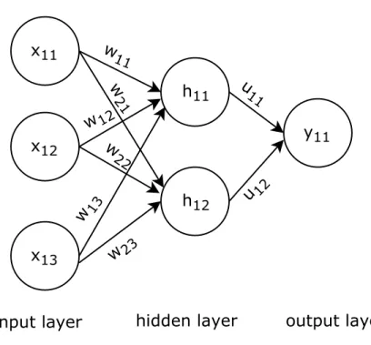
Figure 2.1 represents a sample neural network architecture. To give some context about nomenclature used in neural networks: any neural network architecture consists of neurons (also referred as units) and connections between neurons which are represented by circles and edges respectively. The way neurons are stacked is referred as neural network architecture. Each neural network architecture is made up of 3 kind of layers. The first layer is called as input layer, last layer is called as output layer and all the other layers between input and output layer are referred as hidden layers. In the sample architecture there is only one hidden layer but usually there are multiple hidden layers. All the neurons in hidden layers and output layer are computational units whose values depend on output of neurons

(18)

Figure 2.1: A sample neural network architecture with 3 neurons in input layer, one hidden layer with 2 neurons and 1 neuron output layer.

in preceding layer. If you notice every neuron in all the layers except input layer is connected to every neuron in preceding layer but this is not the case in all the architectures.

Neurons in the input layer are initialized by features xi. All neurons in hidden layers and output layer are computational units whose values depends on neurons in the preceding layer. To give an example value of neuron h12 depends on x11, x12, x13 neurons, value of y11 depends on h11, h12. Let x1..xm be inputs to neuron j in a layer then output of the neuron is given as hj =a( m X n=1 wjixi+bj) (2.1)

where wji is weighted connection between jth neuron and bj is bias of neuron j, a is nonlinear function which is also referred as activation function. Tanh, ReLU are couple of famous activation functions. More about activation functions and different activation functions is stated in [33]. Output of all neurons can be calculated this way.

(19)

Output of neurons in all layers except in input layer depend on preceding layer. The training begins by calculating activations of neurons in first hidden layer and this output is further propagated to successive layers. This process of propagation is called as forward propagation. After each forward propagation step, value of y’ can be calculated as y_i0 =

f(xi) where f is a non-linear function that is parameterized by weight terms for each of the connection between neurons and bias terms for each node. The objective function to train the neural network depends on learning task. In case of classification objective function is to minimize classification error. For instance, classification error can be modelled as mean squared error between the actual label yi of featurexi and estimated label yi0. The standard backpropogation algorithm is used to train neural networks. A thorough information on backpropogation is given [32].

While fully connected neural networks can be used to model non-complex relationship between features and labels there are different problems associated with them. Fully con-nected models do not scale well for high resolution images. For example if there is image which is 100x100x3, then there are 30000 neurons in input layer. As every neuron in hidden layer is connected to every neuron in input later there are hundreds of thousand of weights to learn. This makes scalability a huge problem. Moreover, overfitting becomes a common problem in these models.

2.1.2 Convolutional neural networks (CNNs)

Convolutional neural network architecture takes advantage of spatial structure of the image. Also, architecture is constrained in more sensible way. Difference between CNNs and fully connected architecture is based on 3 concepts: local receptive fields, shared weights, and pooling. In fully connected architecture it is intuitive to visualize pixels as arranged in vertical line. To understand CNN it helps to visualize image as a 2D structure. It is

(20)

reasonable thing to assume that pixels that are structurally close together are more correlated than pixels that are far away from each other. CNNs take advantage of this concept.

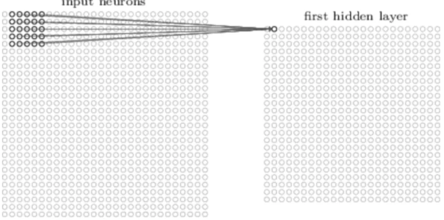
Recall that in fully connected architecture activation of a neuron depends on all neurons in previous layer. Instead in CNNs, value of neuron is calculated using a small region of neuron in the preceding layer. For example given a 28×28 image activation of neuron is may be calculated using 5×5 sub-window. Figure 2.2 showcases this. Neurons in the sub-window affect the activation of neuron and this sub-sub-window is called local receptive field. As neurons are connected to only 5×5 neurons instead of 28×28 neurons lesser number of parameters are involved.

Figure 2.2: Example of a convolutional layer on input of size 28×28.

In fully connected architecture, every neuron had there own set of weights connected to their inputs. It can be seen as each neuron is trying to learn a different filter. In case of CNN weights are shared across different sub-windows. This means that all neurons are learning same filter but at different regions of the image. This mapping is sometimes referred as feature maps and weights associated with this feature maps are called as shared weights or kernel or a filter. Using one set of shared weights we can learn one feature map and in order

(21)

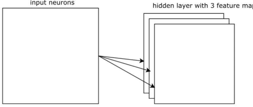
to learn multiple feature maps multiple filters can be used. In figure2.3 there are 3 features maps. Sharing weights gives architecture capability to generalize well.

Figure 2.3: Example of a hidden layer with 3 feature maps.

The last concept is pooling. Pooling takes feature maps and produced a condensed

feature map.This is done in order to simplify information in the output. Pooling layers are generally followed by convolutional layers. For example, each neuron in the pooling may be summarizing information in 2×2 region. There are different functions for pooling max pooling and average pooling being the most common ones. In a typical CNN architecture, multiple convolutional followed by pooling layers are stacked. In conclusion, CNNs have far less number of parameters which makes training comparatively easy. This enables training of deep nets.

2.2 Manual Data Augmentation

Photo-metric and geometric variations on base data is usual way of doing manual data augmentation. While performing rotations, translation, flipping, scaling, shearing fall under geometric variations changing the color palette of an image is the most common way of doing photo-metric variation. Geometric variations can be calculated by applying affine displacements to the images in training data. The new target position of every pixel (x’,y’)

(22)

is calculated with respect to original position (x,y). For example, if we want to shift image to left by 1 then new target location for each pixel is calculated as x’ = x-1, y’=y. If the displacement field is x0 = −y and y0 = x then the image would be rotated clockwise by 90◦. Scaling is little complex due to fact that scaling value could be a non-integer value and requires interpolation to compute new values for each pixel. Taking an example from [7]to explains this process.

Figure 2.4: Given displacement field asx0= 1.75xandy0 =−0.5y, how to compute new pixel value for A located at (0,0). Bilinear interpolation yields 8. Example from [7]

Figure2.4 illustrates how to calculate new pixel values based on the displacement fields. In this example location of A is (0,0) and displacement value for A isx0 = 1.75 andy0 =−0.5, hence the diagonal arrow. 3,7,5,9 are the pixel values of images that need to be transformed, at the locations (1,0), (2,0), (1,-1), (2,-1) respectively. The new pixel value for A in the generated image will be the pixel value from original image at location (1.75,-0.5). Many algorithms exist to evaluate new pixel values : bilinear interpolation, bicubic and spline interpolation. Of these bilinear interpolation is the simplest and used here to illustrate

(23)

Figure 2.5: Typical geometric transformations.

interpolation process.Interpolating the value horizontally, followed by interpolating the value vertically will yield new pixel value. Before calculating these interpolations, we need to calculate the location of where arrow ends with respect to the square it ends in. Assuming bottom left (where 5 is located) as origin, coordinates in the square are (0.75,0.5). New values for horizontal interpolation are: 3 + 0.75 x(7−3) = 6 and 5 + 0.75 x(9−5) = 8. The vertical interpolation yields new pixel value for A which is 8 + 0.5 x(6−8) = 7. In similar fashion, computation is done for all the pixels in the image. All pixel locations outside image are assumed to have a fixed background value (e.g. 255). Figure2.5 represents typical manual geometric transformations

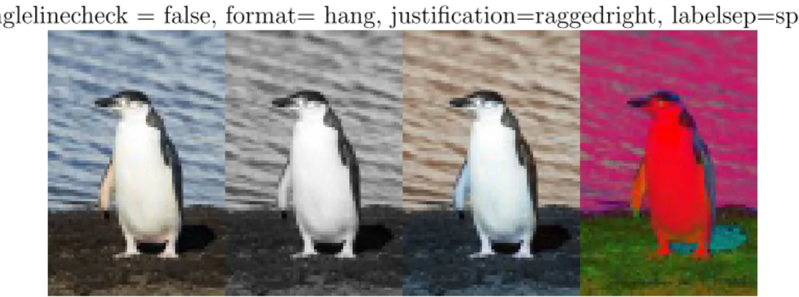
Images are usually represented in RGB format but there are hundreds of other color spaces and conversion methods that can be used to transform from one color space to another. Each color space differs from other in a way that they represent a color, for instance in BGR a color is represented by percentage of red, green, and blue hues where as in HSV a color is represented by combination of hue, saturation and value. Each color space has its own advantages. HSV for example separates color from intensity and this color space can be used to build a model which is robust to lighting changes and/or shadows. Most wildly used conversions are from RGB to Gray, RGB to HSV, RGB to BGR and we will look at algorithms to achieve these conversions. To convert BGR to Gray scale, there exists many

(24)

singlelinecheck = false, format= hang, justification=raggedright, labelsep=space

Figure 2.6: Different color spaces on same image. From left to right BGR,GRAY,RGB,HSV color spaces.

algorithms of those we will explore 3 common and popular methods. The first one is a lightness method which simply averages most prominent and less prominent channel value, second is an average method which just averages all channel values, luminosity is the third method which is similar to average method except it is a weighted average of channel values. Human eyes are more sensitive to green color and hence has highest weight. Equations 2.2, 2.3, 2.4 represent formulas for lightness, average, and luminosity methods respectively.

Y = [max(R, G, B) +min(R, G, B)]/2 (2.2)

Y = [R+G+B]/2 (2.3)

Y = [0.299∗R+ 0.587∗G+ 0.114∗B]/2 (2.4)

Conversion from RGB to Gray is fairly simple where as conversion from RGB to HSV is slightly complicated. More information on the conversion algorithm is given in wiki page [34].

Many open source libraries like opencv[29], matplotlib[30]and deep learning frameworks like keras [31] have built in methods to perform both photo-metric and geometric

(25)

transfor-mations making manual data augmentation easiest and efficient way to avoid overfitting. Researchers have reported pretty good results using manual data augmentation techniques and can be applied to most use cases. But in some scenarios using data augmentation tech-niques we may end up labeling images incorrectly which will just confuse the model instead of helping the model to better learn. To illustrate this consider MNIST[19] dataset, there is a very high probability that image ”6” looks like ”9” by applying rotation, same can happen when flipping is applied on traffic signs, left arrow will be labeled as right arrow and vice versa.

2.3 Generative Adversarial Networks

Generative adversarial networks (GANs) have been first introduced by Goodfellow et al. [20] in 2014 and gained lot of attention in the past few years. GANs are generative models via adversarial process. GANs contain two models a generator G model and a discriminator

D model. The goal of generator is to learn distributionpg of particular data setpdata where as the aim of discriminator is to differentiate if the data is from real distribution pdata or from distribution learned by the generatorpg. In terms of images, discriminator is trying to distinguish between real and synthetic images while generator is trying to generate natural looking images. It can be seen as zero-sum or minimax game where generator is trying to fool discriminator while discriminator is trying not to get fooled by the generator.

In a simple GAN, input to generator is a noise vector z taken from a distributionpz(z) and outputs an image G(z) where as discriminator takes this image G(z) or a image xfrom the distribution pdata as input and outputs a scalar D(x) which represents the probability that x came from data rather than pg, where G,D are differential functions represented by multilayer perceptrons with parametersθ(g) and θ(d) respectively. The training strategy for discriminator is to maximize the probability of assigning correct label to samples from pdata

(26)

Figure 2.7: Samples generated by GANs in[20]. Rightmost column shows nearest training examples of neighbouring samples.

and pg where as goal of generator is to minimize log(1−D(G(z))). In other words, this is a two player minimax game with value function V(G, D) :

min G

max D

=Ex∼pdata(x)(log(D(x)) +Ez∼p(z)(log(1−D(G(z))) (2.5)

When generator is poor and discriminator is able to distinguish generated data from real data with high confidencelog(1−D(G(z))) suffers from vanishing gradient descent problem. In other words,log(1−D(G(z))) saturates. In practice it is suggested[20]to use maximizing

log(D(G(z)) as loss function for generator rather than minimizinglog(1−D(G(z))) to provide sufficient gradient for generator to learn.

The result of generator is the model distribution pg and this model can be used to

es-timate samples. Figure 2.7 show cases generated samples for MNIST [19] and CIFAR-10

[16] datasets. Note that generator produced reasonable samples with MNIST data set but with CIFAR-10 samples created are blurry. GANs are known to be very unstable to train resulting in generators that produce useless outputs. This problem is explored extensively. A laplacian pyramid extension to generative adversarial networks [21] had some success which produced higher quality images, but the objects in samples looked wobbly because of the noise introduced in chaining multiple model. On the other hand, deep convolutional generative adversarial networks (DCGAN)[22]achieved good results mostly because the ar-chitecture was stable to train in most settings resulting in quality samples. In DCGAN, both

(27)

the models generator and discriminator are convolutional neural networks(CNNs) instead of multilayer perceptrons.

DCGAN [22] was developed in order to stabilize training GANs and generate sensible output. Even though DCGAN architecture does a good job, using class labels in training

GANs further stabilizes the network. CatGAN [24], LabelGAN [25], AC-GAN [27],

AM-GAN [26] all these GAN models made use of label information which improved generation

quality and stability.

LabelGAN

In a simple GAN model, discriminator is a two class classifier which distinguishes a real image from a fake one. In this setting given a data point x, discriminator outputs a scalar D(x) that lies within a range of 0 to 1 and if value ofD(x) is less than 0.5 then x is classified as a generated image otherwise as a real image. In LabelGAN[25], this framework is extended to build a classifier with more than 2 classes. Given a dataset with K classes, discriminator is (K+1) classes classifier where (K+1)th class corresponds to generated images. Discriminator outputs a (K+1) dimensional logit vectorD(x) from which class probabilities can be obtained by applying softmax function. Suppose x is input to the discriminator then probability that x belongs to class j is given by

pmodel(y=j|x) = exp(lj) k+1 X i=1 exp(lk) , j ∈ {1...K+ 1} (2.6)

where lj is jth entry in (K+1) dimensional logit vector D(x). The probability that x is fake is given by pmodel(y = K + 1|x) corresponding to 1−D(G(z)) in equation 2.5. Replacing this in equation the value function of minimax game becomes V(G, D) :

min G

max D

(28)

Replacing D(G(z)) with pmodel(y=K+ 1|x) the loss function of generator is then defined as

Lgen =−Ex∼pg[log(1−pmodel(y=K+ 1|x)] (2.8)

note that K+1

P

j=1

{pmodel(y = j|x)} = 1 and {1−pmodel(y = K + 1|x)} = K P

j=1

{pmodel(y = j|x)} replacing this in equation 3.4 gives us below equation

Lgen =−Ex∼pg[log K X

j=1

pmodel(y=j|x)] (2.9)

and the loss function of discriminator is given as

Ldis =−Ex,y∼pdata(x,y)[logpmodel(y|x)−Ex∼pg[logpmodel(y=K+ 1|x)] (2.10)

max

θd

(Ex,y∼pdata(x,y)[logDθd(y|x))] +Ez∼p(z)[logDθd(y=k+ 1|Gθg(z))] ) (2.11)

max θg (Ez∼p(z)logDθd(y=c|Gθg(z))) (2.12) max θg (Ez∼p₍_z₎log K X j=1 Dθd(y=j|Gθg(z))) (2.13) Gθg(z) (2.14) min z0 x−G_θ_g(z0)) 2 2 (2.15)

If we look at the generator’s loss, objective of generator is to maximize the probability that sample belongs to one of the k classes. In other words, gradient of generator’s loss is used to refine samples to one of the k classes. This is why class label information makes training GANs more suitable.

(29)

Figure 2.8: Overlaid gradient problem[26]. Suppose there are two classes and generated sample is encouraged to one of the class, the averaged gradient may not belong to none of the classes.

AM-GAN

As each sample is encouraged to be one of the k classes, making gradient of each sample a weighted average of multiple label predictors due to which this gradient can point to none of the classes [26]. This problem is referred as overlaid gradient problem and figure 2.8 illustrates this. AM-GAN addresses this problem by assigning each sample a specific target class c. A class label c is passed to generator in addition to noise z and loss function is formulated as

Lgen =−Ex∼pg[logpmodel(y=c|x)] (2.16)

while the loss function of discriminator is unchanged. This solves overlaid-gradient descent problem.

Our goal is to test a simple hypothesis: creating more data using GANs achieves better classification accuracy than traditional augmentation techniques. In order to test this hy-pothesis we need to perform class label-preserving transformation using GANs. Most of the work on GANs is based on using unlabeled data generated from GANs to improve accuracy for instance in semi-supervised learning [25]. In an ideal scenario generator learns distribu-tion of the data pdata and produces samples that cannot be distinguished by discriminator.

(30)

Then in architectures like LabelGAN where discriminator act as perfect classifier can be used to label generated data but in practice this is not possible. So we propose a new framework to create more data while preserving the class labels.

During training phase three different models are trained sequentially: model 1 is a GAN model which maps variable z inpz low dimensional spaceRk to variableG(z) in high dimen-sional space Rn _{where G is a function as described in 3.1.2, model 2 takes an image x from} data distribution pdata ∈ Rn and maps it to latent variable z in pz distribution using the distribution learned by DCGAN and finally network 3 is the main network used to perform a specific task (in this paper classification of images). Model 3 is the main model designated to achieve specific supervised learning task for example hand writing recognition, optical character recognition, object recognition etc. In this research we build a neural network model to recognize objects in the digital images. Chapter 3 explain these models in detail.

(31)

CHAPTER 3. METHODOLOGY

To describe briefly, our thesis contains two principal components: generating label

pre-serving samples using GANs, common data augmentation methods (component-1) and to

test a simple hypothesis (component-2): samples generated from GANs are more realistic and hence yield better object detection accuracy than samples generated by applying tra-ditional data augmentation techniques. Section 3.2.1 talks about architecture used to train our generative adversarial networks. This section further describes framework employed to generate samples from GANs with labels. Additionally, in order to test out hypothesis we create data using common traditional techniques and further details about this are men-tioned in Section 3.3. Finally, section 3.4 discloses object detection architecture employed to test hypothesis.

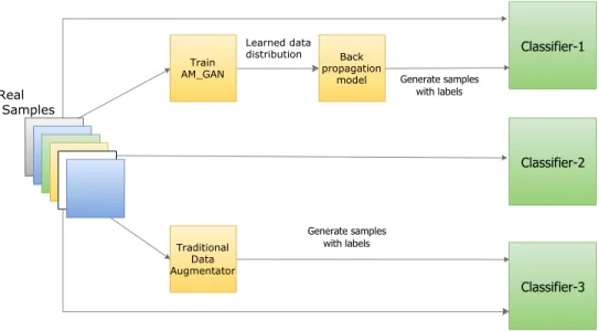
To provide context, here is a high-level overview. AM-GAN loss function is employed to learn the underlying distribution of the data. After training the GAN, we build a simple back propagation model which learns to project given data sample on to latent space. We then randomly perturb the latent variable learned for that sample, pass it back through generator to produce augmented samples of the original sample. We repeat this process with different data samples to create more data. To test the hypothesis we also create data using traditional data augmentation techniques. Finally, a classifier is trained with three different databases. This is to analyze in which setting does the classifier perform better. The first database is the original data, second one is original data plus generated samples from GANs while the last one is original data supplemented with data created using traditional augmentation techniques. Figure 3.1 illustrates this pipeline.

(32)

Figure 3.1: This figure exposes different modules in the pipeline. To the left is component-1 that involves generating data whereas to the right iscomponent-2 whose agenda is to test which classifier is best

3.1 Data Preprocessing

Data pre-processing is a necessary step in order to deal with different distortions in the images. We follow 3 basic image pre-processing steps and these steps are outlined below:

1. To deal with varying image sizes in the dataset, we began by finding maximum height

h and width w of the images in the dataset. The size of the image is then calculated as s = max(h, w). Then we padded all the images in the dataset to s-by-s. Images are prepossessed to be square to make training of GANs stable and scalable. At this point all images contain s-by-s pixels. Considering there are n images in dataset with each image having c number of color channels we get n matrices of pixelsx(i) _∈_Rs×s×c where i=1...n

2. Most of the times, real world datasets contain images of very high resolution which makes training on these datasets not feasible. In order to avoid this, depending on

(33)

the size of the image we re-size images to downscale the size of image by some factor m. This results in n matricesx(i) ∈R(s/m)×(s/m)×c where i=1...n (For example, images in GDXRay [35] data set after the first step images were of size 2200x2200. By down scaling images by a factor of 20 brings down size to 110x110)

3. Following an old convention, we normalize each pixel in the image (in range 0 to 255) in RGB by subtracting 127.5 and by dividing by 128. This process outputs a normalized vector where each pixel value ranges from -1 to 1.

3.2 Data Augmentation using GANs

In this section, we elaborate more on data augmentation using GANs module. At the most fundamental level, number of convolutional layers in both generator and discriminator is calculated based on image size after data pre-processing. Equipped with the data distribution learned by the generator, we further train a gradient-based model by back propagating L2 loss to produce samples.

3.2.1 Training GANs

Recall that goal of generator is to construct a map from variable z(i) in latent space Pz to a image x(i) in given data distribution.

x(i) =f(z(i)) (3.1)

On the other hand discriminator takes an image x(i) _{as input and output a vector} _o(i)_{. The} output vector o(i) _{can represent one of the following:}

1. A 2-dimensional vector which represents the probability that image is fake and prob-ability that image is real

(34)

2. Given that images in dataset belong to k different classes, output vector o(i) is k+1 dimensional vector. The first k entries represent the probability that image is from one of the k classes whereas (k+1)th entry represents probability that image is fake. Attempts to model GANs using CNNs to generate high resolution images have been un-successful. Authors of APGAN [21] took the route of generating low resolution images and iteratively up-scaling the generating images. After exploring and experimenting extensively

authors of DCGAN [25] came up with a framework that’s is suitable to train GANs that

produce high resolution images. This framework also resulted in stable training across a range of datasets. We employ this framework to train GANs. This framework is based on applying three recent changes in the the CNN architectures.

A traditional convention is to have a convolutional layers followed by a pooling layer in each layer of CNN. Pooling is applied in order to down-sample. But it is recently demon-strated that having all convolutional layers and allowing network to learn its own spatial down-sampling increased performance of CNNs. This is the first thing we will employ in our architecture.

A common choice of neural network architecture is to have a block of convolutional neural network layers followed by stack of fully connected layers. The final fully connected generally has a softmax activation function with each node in the layer representing the probability that image belongs to a particular class. Fully connected layers involve lot of parameters causing model to easily over-fit and the common way to avoid this is using dropout. More recently a new technique called global average pooling is proposed which reduces overfitting by reducing number of parameters in the network. Similar to max pooling, global average pooling reduces spatial dimensions. Although, global average pooling is a more extreme on

reducing dimensions. A h × w × d tensor is converted to 1 × 1 × d by simply taking

(35)

probability. This will be the second change in our architecture. Even though global average pooling increased model stability it hurt convergence speed. Authors of DCGAN[25]suggest to connect highest number of features to input and output of generator and discriminator respectively.

A common problem while training GANs is generator collapsing to produce samples from same point. In order to avoid it is suggested to use batch normalization. Batch normalization normalizes input to each unit to have zero mean and unit variance. This enables to deal with problems that arise from poor initialization and also helps addressing vanishing and exploding and other gradient descent problems. This is the third change that is employed in our architecture.

As mentioned above modeling GANs to generate high resolution images is a very unstable process as a result choosing same architecture for both generator and discriminator for different datasets with varying resolutions is nonsensical. That’s is the reason we modelled our architecture in such a way that number of convolutions neural network layers in generator and discriminator depend on resolution of images in the dataset. Number of convolutional layers in generator is calculated as num of layers = log₂(height of image)−2 on the other hand number of convolutional layers in discriminator is calculated as num of layers +1.

Input to generator is a vector which is either taken from uniform distribution or normal distribution. The first layer in generator architecture is matrix multiplication and can be called as fully connected layer. The output of this layer is then reshaped to 4-dimensional tensor. Batch normalization is applied on this 4-dimensional tensor. The resulting tensor serves as a start of convolution stack. and has size n x 4 x 4 x f where n is number of images in batch size and value for this is decided based on heuristics, f is number of convolutional features and is calculated as f = 128*(num of layers-1).

Every convolutional layer except the last one in the stack takes a tensor of the form n × [4*layer number] × [4*layer number] × [f/2layer number−1] as input and outputs a tensor

(36)

of the form n × [4*(layer number+1)] × [4*(layer number+1)] × [f/2layer number] where

layer number = 1...(num of layers-1). It has to be noted that height and width in each layer is up-sampled by a factor of 2 whereas number of features is down-sampled by a factor 2. In each convolutional neural network layer transpose of a convolution is applied in order to upscale with a kernel of size 5-by-5 with a stride of 2 in both horizontal and vertical directions. Batch normalization is applied to output of each convolutional layer before passing as input to successive CNN layer. The last layer in the convolutional stack produces an output that is of size n×s×s× c where s is the size of the image and c is number of channels in the image. In order to avoid sample oscillation and model stability batch normalization is not applied to the last layer. Finally, tanh activation function is applied to the output. The output from the activation function serves as generated samples.

Input to discriminator is a image of size n×s×s× c. Discriminator has one additional convolutional layer than number of layers in generator. The first layer in the architecture is a convolutional layer. In this layer instead of reducing dimensions of input we produce more feature maps. More precisely, output from this layer is a representation of sizen×s×s×64. Dropout is applied to output of this layer to avoid overfitting. All the rest of convolutional layers stacked on top of this take input of the form n × [s/2*(layer number-1)] × [s/2* (layer number-1)] × [64*(layer number-1)] as input and outputs a tensor of the form n × [s/2*(layer number)] × [s/2*(layer number-1)] ×[64*layer number] wherelayer number = 2...(num of layers+1). In generator height and width in each layer is up-sampled by a factor of 2 and number of features is down-sampled by a factor 2. On the other hand in discriminator height and width in each layer is down-scaled by 2 and number of features is up-scaled by factor 2. It is to be noted that architecture is modelled in such a way that highest number of convolutional layers are connected to input and output of generator and discriminator respectively. From second convolutional layer, convolution is applied to downscale with a kernel of size 3-by-3 with a stride of 2 in both horizontal and vertical directions. As

(37)

Figure 3.2: Generator architecture for dataset with images of size 32×32×3.

Figure 3.3: Discriminator architecture for dataset with images of size 32×32×3.

was the case in generator, batch normalization is applied to output of each convolutional layer. Additionally, dropout is applied in all the layers except in the last convolutional layer before passing as input to successive CNN layer. The last layer in the convolutional stack produces an output that is of size n×4×4×64∗(num of layers+ 1) . Global average pooling is applied to output from last convolutional layer resulting in representation of size

n×1×1×64∗(num of layers+ 1). The final layer in the architecture is fully connected layer, output from this layer is a matrix of size n×(k+ 1). Soft-max activation function is applied on output from this layer which predicts the probability of an image belonging to k+1 different classes.

The figures 3.2 and 3.3 represent a sample architecture for generator and discriminator for images of size 32×32×3 which belong to k-different classes.

(38)

3.2.2 Gradient-based model to reconstruct latent space variable of a sample There is no existing framework that can correctly label the generated samples. Generator maps a variable in latent space to real-looking images. In order to produce additional data belonging to a class, we took the route of training a gradient-based model that takes as input an image from this class and produces invert mapping of this image: a latent space variable. The latent space variable is then perturbed to produce additional images that belong to this class.

For any given image x there exists a latent space variable z such that x=pg(z). In order to learn z, we initialize a new vector z0 that has same shape as z. Then z0 is iteratively updated using gradient descent in order to make pg(z0) move closer to pg(z). The L2 loss is employed for the optimization. The loss function is given as:

min

z0 k(pg(z)−pg(z

0

))k2₂ (3.2)

3.3 Data Augmentation using traditional techniques

Even though there exists lot of manual data augmentation techniques as described in section 2.2 we employ only few of them to test our hypothesis. To be more precise, we perform translation, rotation, and a combination of translation and rotation on the images in original dataset. Before data pre-processing original images in the dataset are used to perform data augmentation. The algorithm 2 explains steps involved more clearly. Then, data pre-processing is performed as described in starting of the chapter-3.

(39)

Algorithm 1: Data Augmentation using GANs Input : Z = {z1, z2, ...zn}with zi = (xi, yi) Output: Z’ = {z₁0, z₂0, ...z_m0 } where m>n

1 Z0 ← {} ;

2 Initialize the weights in discriminator and generator ; 3 for i←0 to num of iterations do

4 update discriminator weights in order to minimize discriminator loss using

back-propagation algorithm ;

5 update generator weights in order to minimize generator loss using

back-propagation algorithm ;

6 for i←0 to num of classes do 7 foreach image x in ith class do

8 using gradient-based model learn inverse mapping z of image x ;

/* augmentation size is size by which number of training examples

has to be up-scaled */

9 for j ←1 to augmentation size do

10 produce z0 by randomly adding noise ∆z to z ;

11 produce image x0 aspg(z+ ∆z) ;

(40)

Algorithm 2: Data Augmentation using manual augmentation techniques Input : Z = {z1, z2, ...zn}with zi = (xi, yi)

Output: Z’ = {z₁0, z₂0, ...z_m0 } where m>n

1 Z0 ← {} ;

2 for i←0 to num of classes do 3 foreach image x in ith class do

/* augmentation size is size by which number of training examples

has to be up-scaled */

4 for j ←0 to augmentation size / 3 do

/* one third of augmented data is produced by translating

images */

5 ∆x = random number between (1,10) ;

6 ∆y = random number between (1,10) ;

7 produce x0 by translating image x with (∆x, ∆y ) displacement ;

8 add (x0,i) to Z0

9 for j ←0 to augmentation size / 3 do

/* one third of augmented data is produced by rotating images */

10 ∆θ = random number between (-15,15) ;

11 produce x0 by rotating image x with angle ∆θ ;

12 add (x0,i) to Z0

13 for j ←2∗(augmentation size/3) to augmentation size do

/* one third of augmented data is produced by a combination of

translation and rotation */

14 ∆x = random number between (1,10) ;

15 ∆y = random number between (1,10) ;

16 ∆θ = random number between (-15,15) ;

17 produce x0 by translating image x with (∆x, ∆y ) displacement and

rotating image with angle ∆θ ;

(41)

3.4 Object Detection

As mentioned in the starting of this chapter, our goal is to test which data augmentation techniques perform better and not to achieve state of the art results on object detection. That is the reason we employed a relatively simple model which enables training on different datasets and testing easier process. The model has two convolution layers followed by a fully connected layer. We used traditional architecture where each convolutional layer is followed by a spatial pooling layers. Output from the spatial pooling layer is fed into fully connected layer, another fully connected layer is stacked on this layer which performs k-class classification (given there are k number of classes in the dataset.)

The input to first layer consisted of batch of images. For every 5-by-5 sub-window we computed activation. By evaluating over entire image using a sub-window of size 5-by-5 with a stride 1, we calculated activation of all neurons in the hidden layer. We calculated 32 such feature maps in this layer. We next introduced max pooling layer, which reduced number of dimensions as well as introduced transitional in-variance to some extent. We used a grid of size 2-by-2, where we took max of 4 blocks arranged in this grid. Another convolutional layer followed by pooling layer is stacked on output from first layer. As was the case 5-by-5 window with stride 1 is used for convolution. In this layer we generated 64 feature maps. After performing convolution 2-by-2 grid is used for max pooling layer. Matrix multiplication is applied on output from this layer which can be called as fully connected layer. We introduced another fully connected layer on top of the first fully connected layer. Output from this layer is passed to softmax function which gives the probability of an image belonging to k-different classes. The stochastic gradient algorithm is used to train the weights involved in the network. As there are huge number of weights involved in the network, a efficient process is required to calculate gradients. The famous back-propagation is employed to compute gradients in an efficient way.

(42)

CHAPTER 4. EXPERIMENTS

In this chapter, we describe our experiments on object detection using data augmenta-tion techniques using manual augmentaaugmenta-tion methods and using neural augmentaaugmenta-tion more precisely using GANs. In addition, we show how our system compares to manual data

aug-mentation methods. For all these experiments, we used CIFAR-10 [16] and MNIST [35]

datasets.

Before proceeding to experiments, we briefly describe characteristics of the datasets. CIFAR-10 is a standard benchmark dataset for object detection systems. The CIFAR-10 images are subset of 80 million Tiny images dataset [36] that are labelled. The dataset includes images that belong to 10 different classes. To be more precise, all the images belong to one of Airplane, Automobile, Bird, Cat, Deer, Dog, Frog, Horse, Ship, and Truck classes. It has to be noted the classes are mutually exclusively. This means that there is no overlap between any two classes for example automobile class contains images of sedans, SUVs etc on the other hand truck contains only big trucks. The CIFAR-10 dataset consists of 60000 32x32 colour images, with 6000 images per class. The dataset is divided into training and testing data. There are 50000 images in training and 10000 images in testing data. On the other hand, MNIST dataset contains images of handwritten digits. There are 70000 handwritten digit in the MNIST database. The images are of size 28x28 that belong to 10 different classes0, 1, 2,3,4, 5,6,7, 8, and9. There are 50000 images in training and 10000 images in testing data. Some examples of CIFAR-10 datasets are illustrated in and some examples MNIST dataset are illustrated in Figure 4.2. All the images in both the datasets are of same size so no much data pre-processing was required except for normalizing images as described in step-3 in section 3.2.

(43)

Figure 4.1: Sample examples from CIFAR-10 dataset[16].

Figure 4.2: Sample example from MNIST dataset [19].

Recall that our experiments are to analyze different data augmentation techniques and not to compare to other object detection systems on these datasets. Refer [28] to see state of the art results on both CIFAR-10 and MNIST datasets.

In order to test different data augmentation techniques, it is required to train multiple models. To make this a feasible process, we employed only subset of these datasets as training data. More precisely, training data for CIFAR-10 and MNIST contains 5000 images with 500 images belonging to each of the 10 classes while keeping the testing data unchanged which has 10000 images.

(44)

4.1 Performance metrics

This section describes our evaluation metrics for object detection system and GANs. To describe briefly accuracy score is used to measure performance of object detection system whereas inception score is used to test performance of GANs.

Recall that, last layer in the object detection system is a fully connected layer on which softmax activation function is applied. The softmax function calculates calculates the prob-ability of an image belonging to K-different classes as:

σ(z)i = ezi K X i=1 ezj for i = 1, ..., K (4.1)

where zj is output from jth neuron in last fully connected layer. Notice that value of σ(z) is value between 0 and 1. The image is assigned a label j given thatσ(z)j ≥σ(z)i for i = 1, ..., K. The label j is often referred as predicted label. After labels are predicted for all the images in the dataset as above accuracy is given as size of intersection divided by the size of the union of two label sets: predicted labels and true labels.

Given there are m images in the dataset then there are m predicted labels and true labels corresponding to each image in the dataset. Assuming labels of n images are predicted correctly accuracy score is given as:

accuracy score = n

m (4.2)

Note that higher the accuracy score better the object detection system.

Inception score [28] is used to compare performance of different GAN models. Inception score is build on the intuition that good GAN model produces a variety of images and each image contains meaningful objects. Combining this two requirements inception score is calculated as:

(45)

where p(y|x) is the conditional distribution of label y on generated image x where as p(y) = R

p(y|x=G(z))dzis overall probability distribution of all generated samples over label y also called marginal distribution. KL is Kullback-Leibler (KL) divergence which calculates how probability distribution diverges from expected probability distribution. The conditional probability p(y|x) is calculated by applying inception model usually a pre-trained model for Imagenet on generated image x. In the case where GAN model which produces high quality images, inception model should be highly confident that there is a single object in the image which means p(y|x) has less entropy. On the other hand if GAN model produces high diversity images then p(y) should be of high entropy.

Code for all the experiments is written in python and we used Tensorflow an open source machine learning framework for building all our models. The GANs are trained on a NVIDIA Geforce GTX 1080 graphics card which took about 6 hours for the training to finish.

4.2 Generative Adversarial networks

We experimented with generative adversarial networks using the CIFAR-10 and MNIST dataset. GANs were trained for 200k,140k iterations on CIFAR-10 and MNIST respectively. The generator and discriminator loss is fixed alternately at each iteration. Adam Optimizer is used for training which takes into account moving averages of parameter which enables taking larger effective steps hence has an advantage of converging faster. It is recommend to reduce learning rate as training progresses for increased performance and to reduce training time. So we used an exponential decay in learning rate. The exponential decay is calculated as

decayed learning rate = learning rate * decay rate ˆ (global step / decay steps)

where learning rate, decay rate, global step, decay steps is initial learning rate, rate of decay, iteration number, and number of decay steps respectively. In our case initial learning is set

(46)

Figure 4.3: CIFAR-10 Samples produced by generator at different level of iteration on five distinct latent variables.

to 0.01, number of decay steps to 20000 and decay rate to 0.1. A batch size of 128 is used in both generator and discriminator. As mentioned in discriminator architecture dropout is used to avoid overfitting. For our experiments, we employed a dropout probability of 0.05. We used a latent space variable of 100 as input to the generator.

We will analyze how GANs train and statistics involved using CIFAR-10 dataset. The idea is that similar statistics will be involved in training of GANs on MNIST. The CIFAR-10 dataset is more versatile dataset covering a broader view of training GANs.

The generator loss is sum of cross entropy loss of generated sample belonging to real class (first term) and cross entropy loss of generated sample belonging to k different classes. Initially probability that a generated belongs to k classes is given as 1/k which means each

(47)

class has equal probability(second term). At start of the training generator produces non-sensible output as shown in figure 4.3. As one would expect, initially the generator loss is very high because of the (first term) in the loss function. As training progresses generator is trying to produce reasonable samples which means samples belonging to any one class should be prominent compared to other classes as a result (second term) in loss starts to dominate. This variations in the generator loss is illustrated in figure 4.5.

The discriminator loss is sum of sum of cross entropy loss of generated sample belonging to fake class plus(first terms), sum of cross entropy loss of real sample belonging to real class plus(second term) and cross entropy loss of real sample belonging to k different classes. The discriminator loss can be seen as a model that is trying to distinguish between real and fake samples and at the same time learning a classifier for the dataset. Not surprisingly, discrim-inator loss decreases with iteration as would any classifier which gets better at classification at each iteration. The evolution of discriminator loss over iterations can be seen in figure 4.6.

An illustration of how inception score changes with number of iterations is given in figure

4.7. The GAN model has an inception score of 8.5 with a standard deviation of ±0.4.

The figure 4.8 shows some of the samples that are produced by the generator. These generated samples are further passes to discriminator to classify these samples. There are a few things to notice here:

1. Notice that 3rd _{figure in third row has a dog with 3 heads. GANs fail to differentiate} number of objects should be present in a particular location, in this case gives more number of heads than they are supposed to be.

2. GANs do not understand holistic structure. For example 4th image in second row or 6th _{image in first row have some weird looking shape of horse.}

(48)

0k 25k 50k 75k 100k 125k 150k 175k 200k 0.605 0.610 0.615 0.620 0.625 0.630 generator loss

Figure 4.5 Generator loss as a variable of it-eration number on CIFAR-10 dataset.

0k 25k 50k 75k 100k 125k 150k 175k 200k 2.10 2.12 2.14 2.16 2.18 discriminator loss

Figure 4.6 Discriminator loss as a variable of iteration number on CIFAR-10 dataset.

0k 25k 50k 75k 100k 125k 150k 175k 200k 7.8 7.9 8.0 8.1 8.2 8.3 8.4 inception score

Figure 4.7 Inception score of the model as a variable of iteration number on CIFAR-10 dataset.

3. Sometimes produces outputs which are hard to tell which class they belong to. For instance, 4th _{image in first row, 2}nd _{image in third row.}

4. The discriminator ends up classifying the samples wrong. The 1st _{image in second row} is labelled dog when clearly it is a Truck. The 6th _{image in third row is labelled Horse} when clearly it an Airplane.

While the first three problems related to generator the fourth problem is partly because of discriminator. As the training progresses, discriminator learns to classify the real samples. If

(49)

Figure 4.8: Samples produced by generator after training. The samples in 3x3 grid to the left are classified as Dog and samples in right 3x3 grid are classified as Horse by discriminator.

the generator produces real samples then discriminator can be used to label these generated samples. As point out in[26] inception score for real samples is 11.24 with± 0.12 standard deviation on the other hand inception score for generated samples is somewhere around 8.5 which means the samples are far from real and hence discriminator fails to classify non-real looking images.

This is the reason we added an additional simple gradient-based model which tries to find closest looking generated sample to a given real image. As we already know the label of the real image, generated sample will be labelled correctly. This also deals with all the other problems mentioned above. Further, in order to produce multiple generated samples of given real sample, latent variable of generated sample is perturbed by a little bit of noise and passed through generator to produce additional samples.

(50)

4.3 Object detection system

The convolutional neural network used for the object detection system is trained in 3 different settings. The first setting is using data from the datasets with out any data aug-mentation. This will give baseline results to compare different data augmentation techniques. In the second setting, additional data is generated using already existing and successful data augmentation methods. This artificially generated data is added to training data. This new bigger training data is used to train the convolutional neural networks. In the third and final setting samples generated from GANs is added to training data. Further, convolutional neural network is trained with this new training data. The network described in section 3.4 is used to train and test and in all the three settings. As results are compared same training parameters are used in all the experiments. The network is trained for 20k iterations with a batch size of 32. The stochastic gradient descent algorithm is used to train the network, as a result randomness has to be taken into account. For this reason training is repeated for 10 times with a different random seed in order to average out randomness. We will refer to this network as object detection system from now on.

4.3.1 Object detection system with no augmentation

The object detection system is trained on two different datasets CIFAR-10 and MNIST. Recall that we considered 5000 images in training data and 10000 images in testing data for both CIFAR-10 and MNIST datasets.

The training accuracy on CIFAR-10 is 85% and testing accuracy is 33%. It is to be noticed that testing accuracy is very low compared to training accuracy. This is because the network contains hundreds of thousands of parameters where as there is only 5000 images to train those parameters and because of this the network is hugely overfitting. In other words,

(51)

with very less data it is easy for the network to memorize images in training data rather than learning low level representation of the objects in the images.

On the other hand a training accuracy of 100% and validation accuracy of 88.88% was achieved. Even though we considered same number of samples as in CIFAR-10 for MNIST dataset, images in MNIST have less number of low-level features as compared to images in CIFAR-10 dataset. This is the reason the very powerful convolutional neural networks yielded very good validation accuracy.

Table 4.1: Classification accuracy on CIFAR-10 with different datasets

Dataset Training

accuracy

Validation accuracy

20k original images in training set 70.81% 37%

20k images artificially generated by manual

augmentation 78% 24.67%

20k images directly sampled from GANs 58.78% 24.26%

20k images artificially generated by GANs(our

approach) 79.13% 30.21%

Table 4.2: Classification accuracy on MNIST with different datasets

Dataset Training

accuracy

Validation accuracy

20k original images in training set 99.89% 95.13%

20k images artificially generated by manual

augmentation 90.89% 27.09%

20k images directly sampled from GANs 52.27% 17.73%

20k images artificially generated by GANs (our

Data augmentation for supervised learning with generative adversarial networks