A Conditional Generative Model for Speech Enhancement

Kent Academic Repository

Full text document (pdf)

Copyright & reuse

Content in the Kent Academic Repository is made available for research purposes. Unless otherwise stated all content is protected by copyright and in the absence of an open licence (eg Creative Commons), permissions for further reuse of content should be sought from the publisher, author or other copyright holder.

Versions of research

The version in the Kent Academic Repository may differ from the final published version.

Users are advised to check http://kar.kent.ac.uk for the status of the paper. Users should always cite the published version of record.

Enquiries

For any further enquiries regarding the licence status of this document, please contact:

[email protected]

If you believe this document infringes copyright then please contact the KAR admin team with the take-down information provided at http://kar.kent.ac.uk/contact.html

Citation for published version

Li, Zheng-xi and Dai, Li-Rong and Song, Yan and McLoughlin, Ian Vince (2018) A Conditional

Generative Model for Speech Enhancement. Circuits, Systems, and Signal Processing . ISSN

0278-081X.

DOI

https://doi.org/10.1007/s00034-018-0798-4

Link to record in KAR

http://kar.kent.ac.uk/66126/

Document Version

Author's Accepted Manuscript

(will be inserted by the editor)

A Conditional Generative Model for Speech

Enhancement

Zeng-Xi Li · Li-Rong Dai · Yan Song ·

Ian McLoughlin

Received: date / Accepted: date

Abstract Deep learning based speech enhancement approaches like Deep Neural Networks (DNN) and Long-Short Term Memory (LSTM) have already demonstrated superior results to classical methods. However these methods do not take full advantage of temporal context information. While DNN and LSTM consider temporal context in the noisy source speech, it does not do so for the estimated clean speech. Both DNN and LSTM also have a tendency to over-smooth spectra, which causes the enhanced speech to sound muffled.

This paper proposes a novel architecture to address both issues, which we term a conditional generative model (CGM). By adopting an adversarial training scheme applied to a generator of deep dilated convolutional layers, CGM is designed to model the joint and symmetric conditions of both noisy and estimated clean spectra. We evaluate CGM against both DNN and LSTM in terms of Perceptual Evaluation of Speech Quality (PESQ) and Short-Time Objective Intelligibility (STOI) on TIMIT sentences corrupted by ITU-T P.501 and NOISEX-92 noise in a range of matched and mismatched noise conditions. Results show that both the CGM architecture and the adversarial training mechanism lead to better PESQ and STOI in all tested noise conditions. In addition to yielding significant improvements in PESQ and STOI, CGM and adversarial training both mitigate against over-smoothing.

Keywords Deep learning·Speech enhancement·Generative model

This work was supported in part by National Natural Science Foundation of China (Grant No. 61273264 and U1613211), and by Science and Technology Department of Anhui Province (No. 15CZZ02007).

Z.-X. Li, L.-R. Dai and Y. Song

National Engineering Laboratory for Speech and Language Information Processing, Univer-sity of Science and Technology of China, Hefei, China. E-mail: [email protected]; [email protected]; [email protected]

Ian McLoughlin

1 Introduction

Speech enhancement aims to improve the quality and intelligibility of speech which is degraded by background noise. Recently, with the emergence of deep learning techniques, Deep Neural Network (DNN) based speech enhancement methods [?,?,?,?,?,?,?,?,?,?,?,?,?] have been demonstrated to outperform classical methods such as spectral subtraction [?] or log-MMSE [?,?]. For ex-ample, in [?], a multi-objective learning framework was proposed to optimize a joint objective function, and mask-based post-processing used to improve performance. Also, in [?], the authors proposed enhancing the noisy and re-verberant speech by learning a mapping to rere-verberant target speech. Most recent works [?,?,?,?,?,?] that employ Long-Short Term Memory (LSTM) [?] to better model the context of long term noisy speech, have achieved even better enhancement results.

However, two issues are still not well addressed in these advances. The first is that the temporal context information, which is characteristic of both noisy and clean speech time sequences, is not fully exploited. In conventional DNN and LSTM based methods, only the temporal context of noisy speech is considered, with the temporal dependency limited by the restricted number of input frames in DNN, or by the finite memory capacity of LSTM.

Meanwhile, the temporal context of output frames (i.e. estimated clean speech), is generally considered to be independent. This is obviously unlike real speech, which does exhibit temporal correlation between frames. Fur-thermore, past frames are not used as an input to the estimation. The sec-ond issue is spectral over-smoothing, generally resulting in muffled enhanced speech [?]. Current DNN and LSTM based methods usually adopt Minimum Mean Square Error (MMSE) as a training criterion, and are widely regarded as regression models. However, the MMSE criterion cannot effectively alleviate spectral over-smoothing, since it is found that smoothing effects often cause square error reduction during estimation [?,?].

To address both issues, we propose a conditional generative model (CGM) for speech enhancement, which will be detailed in Section 2. CGM comprises a generator and a discriminator plus a training scheme. Specifically, we design a novel generator inspired by WaveNet [?] to take full advantage of temporal context information in both noisy and estimated clean speech spectra, and replace conventional MMSE with a more elaborate criterion that can provide a more realistic and accurate estimation. Furthermore, an adversarial training scheme inspired by Generative Adversarial Networks (GANs) [?] is adopted to achieve this.

As far as we know, the first attempt at using GAN for speech enhancement is SEGAN [?], in which a generator directly imports approximately one second of noisy waveform, then outputs a clean waveform of the same length. SEGAN achieved a Perceptual Evaluation of Speech Quality (PESQ) [?] improvement of approximately 0.2 over unprocessed noisy speech. It was a clear demonstra-tion of the potential of GANs for speech enhancement. Unlike SEGAN, our proposed CGM architecture mainly operates in the frequency domain with

context input from both noisy and estimated clean speech spectra. Further-more, CGM can support different generators. In Section 3 we make use of this property to evaluate using conventional DNN and LSTMs as generators within the new architecture. Evaluation in terms of PESQ and Short-Time Objective Intelligibility (STOI) [?] will show that CGM is able to effectively exploit the temporal context information in both noisy and clean speech. Section 4 will detail significant enhancement improvements compared to DNN and LSTM with both the architecture and the adversarial training scheme being shown able to contribute to overall performance. Section 5 will conclude the paper.

2 Conditional Generative Model

As mentioned, CGM is expected to model the conditional distribution of cur-rent clean spectrum, given input (noisy) and past estimated output (clean) spectra:

xt∼pr(xt|xt−1, . . . ,xt−C,yt+F, . . . ,yt, . . . ,yt−P) (1) where xt and yt are the t-th frame of clean and noisy spectra and C, F and P determine the receptive field of past clean spectra, future and past noisy spectra respectively. Unfortunately, the distribution shown in Eq. (1) is difficult to model explicitly because of the high dimensional continuous variable

xt. However, it is possible to model the distribution implicitly according to the principles of the GAN framework. GAN generatorG, estimates thet-th clean frame, ˆxt, as,

ˆ

xt=G(xt−1, . . . ,xt−C,yt+F, . . . ,yt, . . . ,yt−P;θ) (2) whereθrepresents the parameter set ofG, and generatorGimplicitly models a conditional distribution,

ˆ

xt∼pθ(ˆxt|xt−1, . . . ,xt−C,yt+F, . . . ,yt, . . . ,yt−P) (3) When adversarial training converges,pθ tends to converge topr, which means ˆ

xt and xt are expected to come from the same conditional distribution [?]. Therefore, in order to implement this idea, three components of CGM are needed; (i) a generatorGwhich imports both noisy and estimated clean spectra to generate ˆxt; (ii) a discriminator D which distinguishes whether the input is a real spectrum or not; (iii) an adversarial training scheme and a multi-step prediction training strategy.

Conventional DNN and LSTMs can also work as generator Gin the pro-posed architecture, although they would only use noisy spectra y as input. The effectiveness of doing this will be evaluated in Section 3.

It is worth mentioning that in this paper, ‘real spectrum’ or ‘real sample’ refer to the magnitude spectrum of clean speech collected from dataset, while ‘fake spectrum’ or ‘fake sample’ denote the estimated clean speech magnitude spectrum generated byG.

2.1 Generator Architecture

In the experiments of this paper, the sampling rate for all waveforms was 16 kHz, from which magnitude spectra of dimension 257 were computed at 32 ms frame length with 10 ms shift. The generator G imports and outputs

µ-law companded [?] magnitude spectra of noisy and estimated clean speech. In fact, this setting is helpful for our generator, because unlike log magnitude spectra,µ-law companded magnitude spectra lie in the range of [-1, 1], which is more suitable for a feedback-structure model. Our initial experiments also showed thatµ-law companded magnitude spectra performed better than log magnitude spectra.

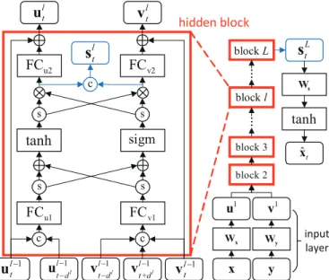
The architecture ofGis shown in Fig. 1 and consists of three parts; input layer, several stacked hidden blocks and an output layer, all described below;

hidden block l t

u

v

s

FC

FC

tanh

u

v

s

Fig. 1 An overview of the generatorGin CGM.xandyrepresent clean and noisy spectra. FC,W, sigm, c, s,⊗and⊕represent full connection, linear transformation, sigmoid ac-tivation, concatenation, equally slicing operation, element-wise multiplication and addition respectively.

1) An input layer processes neighboring clean and noisy spectra at each time step with linear transformation:

u1_t =Wx[xt−1,xt−2] (4)

v1_t =Wy[yt+1,yt,yt−1] (5)

where [.] represents concatenation.

2) L−1 hidden blocks are stacked, as shown in Fig. 1. Hidden blocks are designed with the main consideration that the enhancement of noisy spectra

will benefit from the estimation of clean spectra, and vice versa. F Cu2 and

F Cv2 are two fully connected layers which have the same input and output

dimensions, but use different sets of parameters. This setting follows the design methodology of ResNet [?], where F Cu2 and F Cv2 both correspond to the

second weight layer in the building block. Meanwhile,tanhandsigmare the main components of the gated activation unit, which was firstly introduced in [?] to replace ReLU [?], and was also used in [?]. For outputsul

t orvlt, the connections within each hidden block are symmetric with respect to inputs

ul−1

∗ and vl∗−1. In addition, with the similar conditioning method in [?], ult andvl

tcan be considered as conditional outputs, i.e.

ul_t=f(ul_t−1,ul_t−₋1_dl|v l−1 t+dl,v l−1 t ,v l−1 t−dl), l= 2, . . . , L (6) vl_t=g(vl_t−₊1_dl,v l−1 t ,v l−1 t−dl|u l−1 t ,u l−1 t−dl), l= 2, . . . , L (7)

wheredl _{is the temporal dilation factor for hidden blockl. In this paper, the} dilation is doubled for every hidden block up to a limit and then repeated: e.g. 1,2,4,8,1,2,4,8. The dilation factors are based on the method used in the WaveNet [?] architecture. As long asLanddl_{of all hidden blocks are known,} according to eqns. (4) to (7),C=Σdl_{+ 2 andP =C−1.}

3) As shown in the right part of Fig. 1, output ˆxt is derived from skip vectorsL

t of the last hidden blockL with a linear transformation and atanh activation:

ˆ

xt= tanh(WssLt) (8)

wheresL_t is the concatenation of the two gated activation units shown towards the top of the hidden block structure in the left part of Fig. 1.

There are two main differences between our proposed architecture and WaveNet. Firstly, WaveNet is a time-consuming architecture, for it predicts one waveform sample at a time, and needs many dilated convolution layers to obtain an adequate receptive field. By contrast, our proposed architecture processes each frame with much fewer convolution layers, which means it is likely to work faster than WaveNet. Secondly, the conditioning methods are different. In WaveNet, the linear transformed condition vector is added directly to activation inputs in all layers, while in our proposed architecture, condition vectors are extracted layer by layer.

2.2 Discriminator Architecture

The discriminatorD imports one frame of 257-dimension magnitude spectra, and must determine whether it is from real or fake data. The architecture ofD

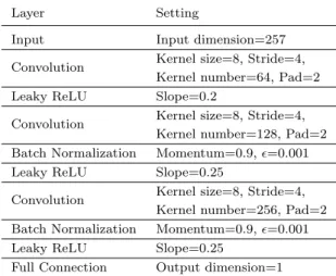
is similar to the DCGAN discriminator [?], and is composed of one-dimensional convolution, leaky ReLU [?], batch normalization [?] and full connection layers. Details of the architecture are shown in Table 1. This architecture cooperates with the adversarial training described in Section 2.3, which is based on the Wasserstein-GAN [?] approach, so the last layer is a linear transformation.

Table 1 DiscriminatorDArchitecture

Layer Setting

Input Input dimension=257 Convolution Kernel size=8, Stride=4,

Kernel number=64, Pad=2 Leaky ReLU Slope=0.2

Convolution Kernel size=8, Stride=4, Kernel number=128, Pad=2 Batch Normalization Momentum=0.9,ǫ=0.001 Leaky ReLU Slope=0.25

Convolution Kernel size=8, Stride=4, Kernel number=256, Pad=2 Batch Normalization Momentum=0.9,ǫ=0.001 Leaky ReLU Slope=0.25

Full Connection Output dimension=1

2.3 Adversarial Training

The two main differences between the proposed architecture and the Wasserstein-GAN system are how it is trained, and how it samples. Firstly, our CGM training criterion is more elaborate. The GAN loss functions forD andGare defined similar to [?] as:

LD=Ez[Exˆt∼pθ(ˆxt|z)D(ˆxt)−Ext∼pr(xt|z)D(xt)] (9)

LG =−EzEˆxt∼pθ(ˆxt|z)D(ˆxt) (10)

where z ={xt−1, . . . ,xt−C,yt+F, . . . ,yt, . . . ,yt−P} is a pair of sequences of clean spectra and corresponding noisy spectra, forming the input ofG. Eqns. (9) and (10) encourage Gto generate realistic spectra, which ideally cannot be distinguished from real ones byD, but they do not indicate the amount of error (or correspondence) between ˆxtand xt. In order to solve this problem,

LG is modified by adding a Mean Square Error (MSE) component to the loss function, which is complementary to GAN loss,

LG=Ez[−αExˆt∼pθ(ˆxt|z)D(ˆxt) +(1−α)Exˆt∼pθ(ˆxt|z),xt∼pr(xt|z) 1 2kxˆt−xtk 2 2] (11) whereα∈[0,1) is a scalar controlling the relative weighting of GAN and MSE loss. Note that αcannot be set to 1 because this will cause MSE loss to be ignored. As a result, G would not generate correct spectra during inference and would fail to enhance noisy speech.

Secondly, a sampling method needs to be defined for eqns. (9) and (11), that incorporates both clean and noisy inputs. To do this, a pair of corresponding clean and noisy spectra sequences,z, are sampled, from whichGgenerates a fake sample ˆxt. Next the real samplext corresponding tozis selected. More details will be given in Section 2.5.

2.4 Multi-step Prediction Training

Using a conventional training procedure [?], a mismatch problem would arise between training and inference stages. This is because, in conventional train-ing, clean spectra ofzare real spectraxt−1, . . . ,xt−C, whereas in the inference stage, these change to predicted spectra ˆxt−1, . . . ,xˆt−C. The errors between the two spectra lead to a mismatch, especially prevalent in low SNR situa-tions. To alleviate this, we adopt a multi-step prediction training strategy. During training,Gdoes look-ahead prediction in sequential time steps. After each spectra is predicted, it is fed back as the next estimated clean input of

G. When multi-step prediction has finished, the loss gradients across all time steps are back-propagated as a batch.

2.5 Complete Training Algorithm

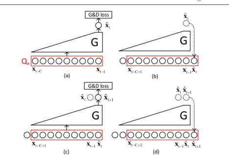
By combining adversarial training and multi-step prediction training described in Section 2.3 and 2.4, we propose the complete training algorithm for CGM, as detailed in Algorithm 1. The main part, line 15 to 22 in Algorithm 1, is illustrated and described in Fig. 2.

It is worth mentioning that, to implement multi-step prediction training, two fixed-size queues, Qx and Qy, are used to store the input sequences of clean and noisy spectra, [xt−1, . . . ,xt−C] and [yt+F, . . . ,yt−P], respectively at current prediction stept. Therefore, the sizes ofQxandQyareCandF+1+P respectively. At the beginning of each step, the input ofG,z, is built with all items of Qxand Qy. Then at the end of each step, the last items ofQx and

Qy are popped out, and the newly estimated clean spectrum is pushed into the front ofQx. Likewise, the next noisy spectrum is pushed into the front of

Qy.

3 Experiments

3.1 Experimental Settings

Experiments employed all 4620 TIMIT [?] utterances for training, along with copies corrupted by 6 SNR levels of 13 types of noise1_{. Meanwhile, 192}

ut-terances from the TIMIT core test set, along with utut-terances corrupted by 6 noise types2 _{at 4 levels of {−5,0,5,10}dB SNR, were used to build the test}

set. Four generative models were used for comparison.

1 _{Noises werecon bin,met mono,off mono,car mono,rai mono,res mono,train,traffic}

from the ITU-T recommendation P.501 database [?] andwhite,factory1,factory2,babble, machinegunfrom NOISEX-92 [?], each at levels of{−5,0,5,10,15,20}dB SNR.

2 _{Matched noises: white from NOISEX-92 database, res mono and con bin from}

ITU-T recommendation P.501 database; Mismatched noises:destroyerops,f16 and m109 from NOISEX-92 database.

G&D loss G&D loss (a) (b) (c) (d)

G

G

G

G

Q

Fig. 2 An illustration of Multi-step Prediction Training in the complete training algorithm of CGM. (a) to (d) mainly shows the procedure of line 15 to 22 in Algorithm 1 whens= 0 ands= 1. The noisy input part is omitted for ease of presentation. Each circle represents one frame of clean or estimated clean spectrum. ”G&D loss” corresponds to the calculation ofLGandLD (line 18 and 19 in Algorithm 1). (a)s= 0,Qx is initialized with all clean spectra, then estimated clean spectrum ˆxtis generated byG.LGandLDat current frame are calculated and accumulated. (b)s= 0, the last itemxt−Cis popped out fromQx, and

ˆ

xtis pushed at the front ofQx. (c)s= 1, ˆxt+1is generated given already changedQx, and another frame ofLGandLDare accumulated. (d)s= 1, the last itemxt−C+1is popped

out from Qx, and ˆxt+1 is pushed at the front ofQx.Qy behaves similarly as Qx, with the difference that clean spectrum is replaced by noisy spectrum. This procedure repeats untils > S−1, with clean spectra inQxgradually replaced by estimated clean spectra. At last,θorφis updated according to line 23 to 28 in Algorithm 1, when allLGandLDare accumulated.

1. DNNwas a baseline deep neural network [?] consisting of 3 hidden layers with 2048 ReLU activation units per layer and a 257-dimensional output layer. Batch Normalization [?] was employed to improve generalization. 2. LSTMwas a baseline LSTM system [?] consisting of 3 hidden layers with

620 cells per layer and a 257-dimensional output layer.

3. CGMS was a short context CGM, sized to match the temporal context of the baseline DNN system. In CGMS,L=3, [d2, d3]=[1,2], and the dimension ofsl

t was 544×2. From Section 2.1, we can see thatC=5 andP=4. 4. CGML was designed to make use of a longer temporal context withL=9

and [d2_{, . . . , d}9_{]=[1,2,4,8,1,2,4,8]. The dimension of s}l

twas 256×2.C was therefore set to 32 and P to 31.

For both DNN and LSTM, 9 frames of noisy log magnitude spectra were concatenated as the input vector at each time step to give a fair compar-ison between methods. Setting F = 4 for the CGMs ensured that all four models imported the same future noisy context of µ-law companded [?] in-put magnitude spectra. In terms of the past noisy spectra, DNN and CGMS

Algorithm 1Complete training algorithm for CGM. Default parameter val-ues used in experiments of this paper:S= 33,K0= 5,µ= 0.00002,m= 256,

c= 0.02,α= 0.5.

Input:

Prediction step size,S;

The number of iteration ofDperGiteration,K0;

Learning rate,µ; Batch size,m; Clipping parameter,c; Weighting parameter,α; Output: Gparameter set,θ; Dparameter set,φ; 1: Randomly initializeθandφ;

2: p= 1;// precords total iteration times 3: whileθhas not convergedo

4: ifmod(p, K0+ 1)6= 0then 5: K=K0;//OptimizeD 6: else 7: K= 1;//OptimizeG 8: end if 9: fork= 1 toKdo 10: ClearDloss:LD= 0; 11: ClearGloss:LG= 0; 12: Sample a batch:{x(_ti₊)_S −1, . . . ,x (i) t−C,y (i) t+F+S, . . . ,y (i) t−P} m i=1.

13: Initialize clean input queue:Qx= [{x(_ti)

−1} m i=1, . . . ,{x (i) t−C} m i=1];

14: Initialize noisy input queue:Qy= [{y(_ti₊)_F}m_i=1, . . . ,{y(_ti)

−P}

m i=1];

15: fors= 0 toS−1do

16: BuildGinput:z={Qx,Qy}; 17: Estimate clean spectra:{xˆ(_ti₊)_s}m

i=1=G(z); 18: AccumulateDloss:LD=LD+m1 Pm i=1[D(ˆx (i) t+s)−D(x (i) t+s)]; 19: AccumulateGloss:LG=LG+_m1 Pmi=1[−αD(ˆx (i) t+s)+(1−α)12kˆx (i) t+s−x (i) t+sk22];

20: Pop out the last item ofQx, push{ˆx_t(i₊)_s}m_i=1at the front ofQx; 21: Pop out the last item ofQy, push{y(ti+)F+s+1}mi=1at the front ofQy;

22: end for

23: if mod(p, K0+ 1)6= 0then

24: Updateφaccording to∇φLDusing RMSProp [?] at learning rateµ; 25: Clipφ:φ= clip(φ,−c, c);

26: else

27: Updateθaccording to∇θLGusing RMSProp at learning rateµ;

28: end if

29: p=p+ 1

30: end for

31: end while

processed the same 4 frames, CGML exploited 31 frames, while LSTM ex-ploited all past frames. Meanwhile the number of parameters in DNN, LSTM and CGMS were all about 13.7 million, and CGML contained fewer, at ap-proximately 12.3 million. As discussed, only the CGMs were able to make use of past clean estimated spectra, with CGMS and CGML importing 5 and 32 frames respectively per step.

Table 2 Exploring the benefit of incorporating clean estimated data as well as noisy input data in the model. PESQ and STOI for various system configurations in different levels of machined and unmatched noise.

Matched noise Mismatched noise

dB SNR -5 0 5 10 -5 0 5 10 Mean PESQ Noisy 1.376 1.716 2.075 2.432 1.487 1.840 2.199 2.544 1.959 DNN 1.967 2.449 2.820 3.084 1.876 2.322 2.686 2.985 2.524 CGMS 2.250 2.684 3.006 3.260 2.018 2.427 2.770 3.081 2.687 LSTM 2.289 2.712 3.006 3.230 1.955 2.415 2.791 3.104 2.688 CGML 2.486 2.900 3.188 3.407 2.006 2.443 2.809 3.131 2.796 STOI Noisy 0.597 0.710 0.812 0.889 0.612 0.717 0.812 0.888 0.755 DNN 0.721 0.821 0.884 0.922 0.683 0.798 0.872 0.917 0.827 CGMS 0.781 0.864 0.916 0.948 0.722 0.825 0.893 0.937 0.861 LSTM 0.791 0.862 0.904 0.931 0.701 0.811 0.881 0.923 0.851 CGML 0.840 0.899 0.935 0.958 0.720 0.827 0.897 0.942 0.878

The adversarial training scheme of Section 2.3, was evaluated with α set to 0.5 in eqn. (11). Conventional MMSE training [?] was evaluated by setting

α= 0 in eqn. (11). The RMSProp algorithm was adopted for the adversar-ial training, with a fixed learning rate of 0.00002. MMSE applied the Adam algorithm [?] with a fixed learning rate of 0.0002. All experiments were im-plemented using MXNet [?], with the enhanced waveform reconstructed from the estimated clean magnitude spectra, using phase from the original noisy speech.

4 Results and Analysis

In this section, results are evaluated to separately identify the benefits of (i) utilizing estimated clean speech as an input, (ii) making use of longer temporal context and (iii) employing adversarial training, before presenting the combined results.

4.1 Utilizing estimated clean speech as input

The hypothesis that exploiting the temporal context in clean estimated speech, in addition to noisy input speech would be advantageous, is tested in this section. To do this we constructed an experiment in which the two CGM structures were operatedwithout _{the benefit of adversarial training, and}

com-pared directly with their matching baseline systems. PESQ and STOI results are shown in Table 2, for both matched and mismatched noise experiments in each system. Each CGM was operated with α = 0 to disable adversarial training. For comparison, scores are also given for un-enhanced noisy input speech.

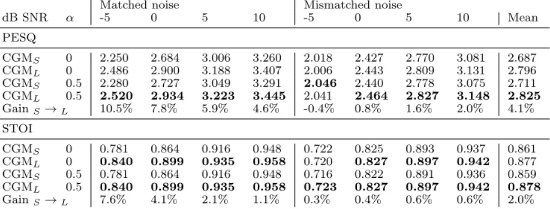
Table 3 Exploring the benefit of increasing temporal context. PESQ and STOI are assessed for various CGM configurations in different levels of machined and unmatched noise, both with adversarial training (α= 0.5) and without (α= 0). The gain in score achieved by the additional temporal context is given as a percentage, for each noise level.

Matched noise Mismatched noise

dB SNR α -5 0 5 10 -5 0 5 10 Mean PESQ CGMS 0 2.250 2.684 3.006 3.260 2.018 2.427 2.770 3.081 2.687 CGML 0 2.486 2.900 3.188 3.407 2.006 2.443 2.809 3.131 2.796 CGMS 0.5 2.280 2.727 3.049 3.291 2.046 2.440 2.778 3.075 2.711 CGML 0.5 2.520 2.934 3.223 3.445 2.041 2.464 2.827 3.148 2.825 GainS→L 10.5% 7.8% 5.9% 4.6% -0.4% 0.8% 1.6% 2.0% 4.1% STOI CGMS 0 0.781 0.864 0.916 0.948 0.722 0.825 0.893 0.937 0.861 CGML 0 0.840 0.899 0.935 0.958 0.720 0.827 0.897 0.942 0.877 CGMS 0.5 0.781 0.864 0.916 0.948 0.716 0.822 0.891 0.936 0.859 CGML 0.5 0.840 0.899 0.935 0.958 0.723 0.827 0.897 0.942 0.878 GainS→L 7.6% 4.1% 2.1% 1.1% 0.3% 0.4% 0.6% 0.6% 2.0%

From this table, we can compare results for CGMS and DNN, which have matching input context lengths, similar numbers of trainable parameters and the same training criteria. The improvement in overall mean PESQ from 2.524 to 2.687, and STOI improvement from 0.827 to 0.861 comes about primarily from the use of additional information contained within the estimated clean speech context.

Similarly we can compare CGML and LSTM, where the CGM uses less temporal context then LSTM, has fewer parameters and the same training criteria, but includes the additional estimated clean speech context. This allows the CGM to improve mean PESQ from 2.688 to 2.796 and STOI from 0.851 to 0.878.

Not only do the overall mean results improve through the use of estimated clean speech context, but the PESQ and STOI are improved for every tested level of noise in both noise conditions. There is thus a clear benefit obtained from incorporating past clean estimated speech frames in the model for sub-sequent frames.

4.2 Increasing temporal context

The two CGMs, with different temporal context lengths (9 and 31 respec-tively), were operated both with and without adversarial training, to determine whether increased temporal context was beneficial to performance. Results are shown in Table 3 for the tested noise levels in both matched and mismatched conditions. A percentage improvement in PESQ and STOI is given for each noise level and condition, as a separate row below the results for each evalua-tion type.

It can be seen that the improvement from additional context is almost (but not quite) identical whenα= 0 to when α= 0.5, but in both cases, the

Table 4 Exploring the benefit of adversarial training. PESQ and STOI are assessed for various system configurations in different levels of machined and unmatched noise, both with adversarial training (α= 0.5) and without (α= 0).

Matched noise Mismatched noise

dB SNR α -5 0 5 10 -5 0 5 10 Mean PESQ Noisy speech 1.376 1.716 2.075 2.432 1.487 1.840 2.199 2.544 1.959 DNN 0 1.967 2.449 2.820 3.084 1.876 2.322 2.686 2.985 2.524 DNN 0.5 2.157 2.633 2.997 3.270 1.918 2.346 2.711 3.028 2.633 LSTM 0 2.289 2.712 3.006 3.230 1.955 2.415 2.791 3.104 2.688 LSTM 0.5 2.335 2.760 3.060 3.293 1.969 2.425 2.803 3.120 2.721 CGMS 0 2.250 2.684 3.006 3.260 2.018 2.427 2.770 3.081 2.687 CGMS 0.5 2.280 2.727 3.049 3.291 2.046 2.440 2.778 3.075 2.711 CGML 0 2.486 2.900 3.188 3.407 2.006 2.443 2.809 3.131 2.796 CGML 0.5 2.520 2.934 3.223 3.445 2.041 2.464 2.827 3.148 2.825 Adv. Gain 3.3% 2.9% 2.6% 2.4% 1.5% 0.7% 0.6% 0.6% 1.8% STOI Noisy speech 0.597 0.710 0.812 0.889 0.612 0.717 0.812 0.888 0.755 DNN 0 0.721 0.821 0.884 0.922 0.683 0.798 0.872 0.917 0.827 DNN 0.5 0.764 0.849 0.902 0.935 0.699 0.806 0.878 0.923 0.845 LSTM 0 0.791 0.862 0.904 0.931 0.701 0.811 0.881 0.923 0.851 LSTM 0.5 0.798 0.866 0.908 0.935 0.702 0.811 0.882 0.924 0.853 CGMS 0 0.781 0.864 0.916 0.948 0.722 0.825 0.893 0.937 0.861 CGMS 0.5 0.781 0.864 0.916 0.948 0.716 0.822 0.891 0.936 0.859 CGML 0 0.840 0.899 0.935 0.958 0.720 0.827 0.897 0.942 0.877 CGML 0.5 0.840 0.899 0.935 0.958 0.723 0.827 0.897 0.942 0.878 Adv. Gain 1.6% 0.9% 0.6% 0.5% 0.5% 0.2% 0.1% 0.2% 0.6%

benefit is greatest at the lowest SNR levels in matched noise but the highest SNR levels in mismatched noise. For example, the additional context improves PESQ by 10.5% at -5 dB SNR in matched noise and by 2.0% at 10 dB SNR in mismatched noise. This result is due to the ability of the underlying model to compensate effectively for familiar noise at even severe levels of corruption (i.e. using the learnt noise temporal context to improve its understanding of the noise in the matched conditions), and use the same ability in mismatched conditions, but applied to the inherent temporal correlation in the speech (i.e. to exploit the longer temporal context of the speech in unfamiliar noise).

4.3 The effect of adversarial training

Table 4 presents results that compare each system, operated with adversarial training (α= 0.5) to the same system without adversarial training (α= 0). Scores are given for un-enhanced noisy input speech, as well as baseline DNN and LSTM systems operating as G in the adversarial training architecture. The ‘Adv. gain’ row along the bottom of the PESQ and STOI sections shows the overall percentage improvement in each score due to the use of adversarial training. Clearly, the main benefits are obtained for the PESQ score in the highest levels of matched noise (3.3%), but it is shown to be beneficial under

Table 5 Performance improvement over baseline for final CGM architectures incorporating adversarial training and temporal context from past estimated clean speech frames.

Matched noise Mismatched noise

dB SNR -5 0 5 10 -5 0 5 10 PESQ DNN→CGMS 15.9% 11.4% 8.1% 6.7% 9.1% 5.1% 3.4% 3.0% LSTM→CGML 10.1% 8.2% 7.2% 6.7% 4.4% 2.0% 1.3% 1.4% Noisy→CGML 83.1% 71.0% 55.3% 41.7% 37.3% 33.9% 28.6% 23.7% STOI DNN→CGMS 8.3% 5.2% 3.6% 2.8% 4.8% 3.0% 2.2% 2.1% LSTM→CGML 6.2% 4.3% 3.4% 2.9% 3.1% 2.0% 1.8% 2.1% Noisy→CGML 40.7% 26.6% 15.1% 7.8% 18.1% 15.3% 10.5% 6.1% 4.4 Summary of improvements

Combining the three factors of adversarial training in the new architecture with the incorporation of temporal context from past estimated clean speech frames, for both long and short temporal context, the overall improvement for each tested noise condition is shown in Table 5. The final row for PESQ and STOI shows the improvement gained over un-enhanced (noisy) speech by the best architecture (CGML with adversarial training). Examining the results, the proposed CGM architecture outperforms the baseline systems on every test case, and provides a very significant enhancement.

4.5 Smoothing effects

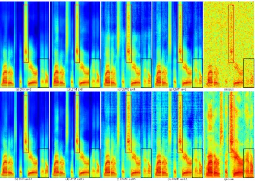
To further study how CGM with adversarial training affects spectral over-smoothing, log domain spectrograms from one utterance in the test set are reproduced in Fig. 3 and Fig. 4 for various conditions. For ease of compar-ison, one unvoiced speech part and one voiced speech part are marked with rectangles respectively in each spectrogram.

Inwhite _{noise conditions (matched noise), when the MMSE criterion was}

employed, from Fig. 3(a)(c), we can see the effects of spectral over-smoothing in both unvoiced and voiced speech parts for DNN and LSTM enhanced speech. However, in Fig. 3(e)(g), CGMs restored some details of both the unvoiced and voiced parts that were lost by DNN or LSTM.

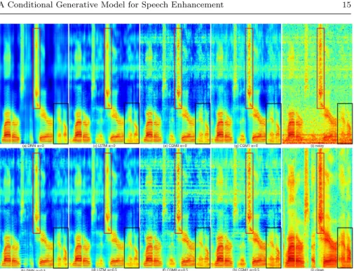
Meanwhile, the effect of adversarial training is shown in Fig. 3 bottom row, namely subplots (b), (d), (f) and (h). For each of DNN, LSTM and CGM, over-smoothing is slightly reduced in unvoiced and voiced parts compared to subplots (a), (c), (e) and (g) in the row above. Results in the m109 _noise

condition (mismatched noise) reveal roughly similar trends, as shown in Fig. 4.

It is worth noting that adversarial training yielded more significant im-provements for DNN and LSTM than for CGMs. This may be due to the fact that over-smoothed spectra generated by DNN or LSTM will result in

larger GAN loss. Therefore, the GAN loss gradients provided by the discrim-inator have a larger effect on the training of DNN or LSTM generators. On the contrary, the CGM itself is able to generate more realistic spectra, which are harder for the discriminator to distinguish. So GAN loss and gradients are smaller than for the DNN or LSTM generators. As a result, adversarial training has a smaller beneficial effect on the CGM. This may also explain why adversarial training obtained better PESQ and STOI improvement for DNN or LSTM than for CGM in Table 4.

These results demonstrate that the adversarial training scheme and the CGM architecture are both beneficial for alleviating spectral over-smoothing, while thecombination_{of both CGM architecture and adversarial training}

per-form even better. This is very much in line with the numerical PESQ and STOI results.

Fig. 3 Spectrograms of one utterance from the test set, showing original clean, noisy and all enhanced versions. The clean utterance was corrupted bywhitenoise (matched noise) at SNR = 0 dB. PESQs for these utterances are: (a) 2.404; (b) 2.462; (c) 2.573; (d) 2.696; (e) 2.683; (f) 2.714; (g) 2.842; (h) 2.891; (i) 1.327. A voiced and an unvoiced region have been outlined with rectangles in each processed spectrogram.

4.6 Overall comparison of various methods

Apart from DNN, LSTM and our proposed methods, a model trained ac-cording to [?], denoted here as Multi-Obj, was also included for

compari-Fig. 4 Spectrograms of one utterance from the test set, showing original clean, noisy and all enhanced versions. The clean utterance was the same as in Fig 3, and was corrupted by m109 noise (mismatched noise) at SNR = 0 dB. PESQs for these utterances are: (a) 2.511; (b) 2.531; (c) 2.573; (d) 2.568; (e) 2.693; (f) 2.675; (g) 2.764; (h) 2.798; (i) 2.074. A voiced and an unvoiced region have been outlined with rectangles in each processed spectrogram.

son. Like DNN, Multi-Obj consisted of 3 hidden layers with 2048 ReLU ac-tivation units per layer. The input comprised a context of 9 frames of 257-dimensional log magnitude spectrum and 41-257-dimensional Mel-Frequency Cep-stral Coefficient (MFCC) of noisy speech, i.e. an input vector dimension of 9×(257 + 41) = 2682. The outputs were one frame of 257-dimensional log magnitude spectrum and 41-dimensional MFCC of estimated clean speech, plus one frame of 257-dimensional Ideal Binary Mask (IBM) [?]. Other set-tings followed [?]: Dropout, mean and variance normalization and Adam al-gorithm were applied for training, while batch normalization was not used. During inference, the post-processing method proposed in [?] was adopted.

Table 6 presents the comparison of model size (in terms of number of parameters), computational complexity (in terms of number of multiplication for estimating per frame of clean spectrum), mean PESQ and STOI of various methods. As discussed in Section 4.3, adversarial training (α=0.5) improved PESQ and STOI without increasing model size and computational complexity. For example, adversarial training raised the PESQ of DNN from 2.524 to 2.633, and STOI from 0.827 to 0.845. Moreover, CGML α=0.5 achieved the best PESQ and STOI, with the smallest model size and computational complexity.

Table 6 Comparison of various methods, in terms of model size, computational complexity, mean PESQ and STOI. Multi-Obj was trained according to [?].α=0 andα=0.5 denote as without and with adversarial training respectively.

Model Model size Computational complexity PESQ STOI (million) (multiplication per frame)

Noisy speech – – 1.959 0.755 DNNα=0 13.7 1.37×107 _{2.524 0.827} DNNα=0.5 13.7 1.37×107 _{2.633 0.845} LSTMα=0 13.7 1.36×107 _{2.688 0.851} LSTMα=0.5 13.7 1.36×107 _{2.721 0.853} CGMSα=0 13.7 1.77×107 2.687 0.861 CGMSα=0.5 13.7 1.77×107 2.711 0.859 CGMLα=0 12.3 1.12×107 2.796 0.877 CGMLα=0.5 12.3 1.12×107 2.825 0.878 Multi-Obj 15.0 1.50×107 _{2.634 0.850} 5 Conclusion

This paper has proposed a conditional generative model (CGM) equipped with an adversarial training scheme for speech enhancement. The novel method is designed to exploit temporal context information from the spectra of both noisy and past estimated clean speech, in contrast to conventional schemes that tend to exploit only noisy input speech context. Experimental results re-veal that CGM outperforms conventional DNN and LSTM models in terms of PESQ and STOI. Meanwhile, the architecture of CGM and the adversar-ial training scheme both appear to be effective at alleviating spectral over-smoothing, particularly when operating in conjunction with each other.

In this paper, the discriminator only determines whether its one frame of input magnitude spectrum is from real or fake data, but ignores the context information in the sequence of clean spectra. This characteristic limits the resolving power of the discriminator. Moreover, the generator needsF frames of future noisy spectrum to estimate current clean spectrum, which results in a time delay during inference. While current performance is good, additional experiments on expanded network structures and larger datasets are planned in the future.

References

1. Y. Xu, J. Du, L.-R. Dai, and C.-H. Lee, “An experimental study on speech enhancement based on deep neural networks,”IEEE Signal processing letters, vol. 21, no. 1, pp. 65–68, 2014.

2. ——, “A regression approach to speech enhancement based on deep neural networks,” IEEE/ACM Transactions on Audio, Speech, and Language Processing, vol. 23, no. 1, pp. 7–19, Jan 2015.

3. Y. Xu, J. Du, Z. Huang, L.-R. Dai, and C.-H. Lee, “Multi-objective learning and mask-based post-processing for deep neural network based speech enhancement,”arXiv preprint arXiv:1703.07172, 2017.

4. Y. Wang, A. Narayanan, and D. Wang, “On training targets for supervised speech separation,” IEEE/ACM Transactions on Audio, Speech and Language Processing (TASLP), vol. 22, no. 12, pp. 1849–1858, 2014.

5. X.-L. Zhang and D. Wang, “Multi-resolution stacking for speech separation based on boosted dnn.” inINTERSPEECH, 2015, pp. 1745–1749.

6. Y. Wang, J. Chen, and D. Wang, “Deep neural network based supervised speech segre-gation generalizes to novel noises through large-scale training,”Dept. of Comput. Sci. and Eng., The Ohio State Univ., Columbus, OH, USA, Tech. Rep. OSU-CISRC-3/15-TR02, 2015.

7. D. S. Williamson, Y. Wang, and D. Wang, “Complex ratio masking for joint enhance-ment of magnitude and phase,” inAcoustics, Speech and Signal Processing (ICASSP), 2016 IEEE International Conference on. IEEE, 2016, pp. 5220–5224.

8. X.-L. Zhang and D. Wang, “A deep ensemble learning method for monaural speech separation,” IEEE/ACM Transactions on Audio, Speech and Language Processing (TASLP), vol. 24, no. 5, pp. 967–977, 2016.

9. Y. Zhao, D. Wang, I. Merks, and T. Zhang, “Dnn-based enhancement of noisy and reverberant speech,” inAcoustics, Speech and Signal Processing (ICASSP), 2016 IEEE International Conference on. IEEE, 2016, pp. 6525–6529.

10. Q. Wang, J. Du, L.-R. Dai, and C.-H. Lee, “Joint noise and mask aware training for dnn-based speech enhancement with sub-band features,” inHands-free Speech Commu-nications and Microphone Arrays (HSCMA), 2017. IEEE, 2017, pp. 101–105. 11. J. Du, Y. Tu, L.-R. Dai, and C.-H. Lee, “A regression approach to single-channel speech

separation via high-resolution deep neural networks,”IEEE/ACM Transactions on Au-dio, Speech and Language Processing (TASLP), vol. 24, no. 8, pp. 1424–1437, 2016. 12. T. Gao, J. Du, L.-R. Dai, and C.-H. Lee, “Snr-based progressive learning of deep neural

network for speech enhancement,”Interspeech 2016, pp. 3713–3717, 2016.

13. A. Kumar and D. Florencio, “Speech enhancement in multiple-noise conditions using deep neural networks,”Interspeech 2016, pp. 3738–3742, 2016.

14. S. Boll, “Suppression of acoustic noise in speech using spectral subtraction,” IEEE Transactions on acoustics, speech, and signal processing, vol. 27, no. 2, pp. 113–120, 1979.

15. Y. Ephraim and D. Malah, “Speech enhancement using a minimum mean-square error log-spectral amplitude estimator,”IEEE Transactions on Acoustics, Speech, and Signal Processing, vol. 33, no. 2, pp. 443–445, 1985.

16. I. Cohen and B. Berdugo, “Speech enhancement for non-stationary noise environments,” Signal processing, vol. 81, no. 11, pp. 2403–2418, 2001.

17. J. Chen and D. Wang, “Long short-term memory for speaker generalization in super-vised speech separation,” inProc. 17th Annu. Conf. Int. Speech Commun. Assoc., 2016, pp. 3314–3318.

18. Z. Chen, S. Watanabe, H. Erdogan, and J. Hershey, “Integration of speech enhancement and recognition using long-short term memory recurrent neural network,” inProc. In-terspeech, 2015.

19. F. Weninger, J. R. Hershey, J. Le Roux, and B. Schuller, “Discriminatively trained recurrent neural networks for single-channel speech separation,” inSignal and Infor-mation Processing (GlobalSIP), 2014 IEEE Global Conference on. IEEE, 2014, pp. 577–581.

20. H. Erdogan, J. R. Hershey, S. Watanabe, and J. Le Roux, “Phase-sensitive and recognition-boosted speech separation using deep recurrent neural networks,” in Acous-tics, Speech and Signal Processing (ICASSP), 2015 IEEE International Conference on. IEEE, 2015, pp. 708–712.

21. L. Sun, J. Du, L.-R. Dai, and C.-H. Lee, “Multiple-target deep learning for lstm-rnn based speech enhancement,” inHands-free Speech Communications and Microphone Arrays (HSCMA), 2017. IEEE, 2017, pp. 136–140.

22. F. Weninger, H. Erdogan, S. Watanabe, E. Vincent, J. Le Roux, J. R. Hershey, and B. Schuller, “Speech enhancement with lstm recurrent neural networks and its applica-tion to noise-robust asr,” inInternational Conference on Latent Variable Analysis and Signal Separation. Springer, 2015, pp. 91–99.

23. S. Hochreiter and J. Schmidhuber, “Long short-term memory,”Neural computation, vol. 9, no. 8, pp. 1735–1780, 1997.

24. Y. Xu, J. Du, L.-R. Dai, and C.-H. Lee, “Global variance equalization for improving deep neural network based speech enhancement,” inSignal and Information Processing (ChinaSIP), 2014 IEEE China Summit & International Conference on. IEEE, 2014, pp. 71–75.

25. T. Toda, A. W. Black, and K. Tokuda, “Voice conversion based on maximum-likelihood estimation of spectral parameter trajectory,”IEEE Transactions on Audio, Speech, and Language Processing, vol. 15, no. 8, pp. 2222–2235, 2007.

26. A. van den Oord, S. Dieleman, H. Zen, K. Simonyan, O. Vinyals, A. Graves, N. Kalch-brenner, A. Senior, and K. Kavukcuoglu, “Wavenet: A generative model for raw audio,” CoRR abs/1609.03499, 2016.

27. I. Goodfellow, J. Pouget-Abadie, M. Mirza, B. Xu, D. Warde-Farley, S. Ozair, A. Courville, and Y. Bengio, “Generative adversarial nets,” inAdvances in neural in-formation processing systems, 2014, pp. 2672–2680.

28. S. Pascual, A. Bonafonte, and J. Serr`a, “Segan: Speech enhancement generative adver-sarial network,”arXiv preprint arXiv:1703.09452, 2017.

29. A. Rix, J. Beerends, M. Hollier, and A. Hekstra, “Perceptual evaluation of speech quality (pesq), an objective method for end-to-end speech quality assessment of narrowband telephone networks and speech codecs,”ITU-T Recommendation, vol. 862, 2001. 30. C. H. Taal, R. C. Hendriks, R. Heusdens, and J. Jensen, “An algorithm for intelligibility

prediction of time–frequency weighted noisy speech,” IEEE Transactions on Audio, Speech, and Language Processing, vol. 19, no. 7, pp. 2125–2136, 2011.

31. I. Goodfellow, “Nips 2016 tutorial: Generative adversarial networks,”arXiv preprint arXiv:1701.00160, 2016.

32. C. Recommendation, “Pulse code modulation (pcm) of voice frequencies,”ITU, 1988. 33. K. He, X. Zhang, S. Ren, and J. Sun, “Deep residual learning for image recognition,” in

Proceedings of the IEEE conference on computer vision and pattern recognition, 2016, pp. 770–778.

34. A. van den Oord, N. Kalchbrenner, L. Espeholt, O. Vinyals, A. Graves et al., “Con-ditional image generation with pixelcnn decoders,” inAdvances in Neural Information Processing Systems, 2016, pp. 4790–4798.

35. V. Nair and G. E. Hinton, “Rectified linear units improve restricted boltzmann ma-chines,” in Proceedings of the 27th international conference on machine learning (ICML-10), 2010, pp. 807–814.

36. A. Radford, L. Metz, and S. Chintala, “Unsupervised representation learning with deep convolutional generative adversarial networks,”arXiv preprint arXiv:1511.06434, 2015. 37. S. Ioffe and C. Szegedy, “Batch normalization: Accelerating deep network training by

reducing internal covariate shift,”arXiv preprint arXiv:1502.03167, 2015.

38. M. Arjovsky, S. Chintala, and L. Bottou, “Wasserstein gan,” arXiv preprint arXiv:1701.07875, 2017.

39. T. Tieleman and G. Hinton, “Rmsprop: Divide the gradient by a running average of its recent magnitude. coursera: Neural networks for machine learning,” Technical report, 2012. 31, Tech. Rep., 2012.

40. J. S. Garofolo, L. F. Lamel, W. M. Fisher, J. G. Fiscus, and D. S. Pallett, “Darpa timit acoustic-phonetic continous speech corpus cd-rom. nist speech disc 1-1.1,”NASA STI/Recon technical report n, vol. 93, 1993.

41. ITU, “Test signals for use in telephonometry,” ITU-T Recommendation P.501, Aug. 1996.

42. A. Varga and H. J. Steeneken, “Assessment for automatic speech recognition: Ii. noisex-92: A database and an experiment to study the effect of additive noise on speech recog-nition systems,”Speech communication, vol. 12, no. 3, pp. 247–251, 1993.

43. D. Kingma and J. Ba, “Adam: A method for stochastic optimization,”arXiv preprint arXiv:1412.6980, 2014.

44. T. Chen, M. Li, Y. Li, M. Lin, N. Wang, M. Wang, T. Xiao, B. Xu, C. Zhang, and Z. Zhang, “Mxnet: A flexible and efficient machine learning library for heterogeneous distributed systems,”arXiv preprint arXiv:1512.01274, 2015.