Network Specialization to Explain the Performance of Sparse Neural Networks

(1)

Master’s thesis

Master’s Programme in Data Science

Network Specialization to Explain the

Performance of Sparse Neural Networks

Vili Hätönen

August 13, 2020

Supervisor(s): Dr. Antti Ukkonen, Dr. Joel Pyykkö

Examiner(s):

Professor Teemu Roos

Dr. Antti Ukkonen

University of Helsinki Faculty of Science

P. O. Box 68 (Pietari Kalmin katu 5) 00014 University of Helsinki

(2)

(3)

Faculty of Science Master’s Programme in Data Science Vili Hätönen

Network Specialization to Explain the Performance of Sparse Neural Networks Master’s thesis August 13, 2020 114

Sparsity, Activation Region, Lottery Ticket Hypothesis, Deep Neural Networks, Bent Hyperplanes Recently it has been shown that sparse neural networks perform better than dense networks with similar number of parameters. In addition, large overparameterized networks have been shown to contain sparse networks which, while trained in isolation, reach or exceed the performance of the large model. However, the methods to explain the success of sparse networks are still lacking. In this work I study the performance of sparse networks using network’s activation regions and patterns, concepts from the neural network expressivity literature.

I define network specialization, a novel concept that considers how distinctly a feed forward neural network (FFNN) has learned to processes high level features in the data. I propose Minimal Blanket Hypervolume (MBH) algorithm to measure the specialization of a FFNN. It finds parts of the input space that the network associates with some user-defined high level feature, and compares their hypervolume to the hypervolume of the input space. My hypothesis is that sparse networks specialize more to high level features than dense networks with the same number of hidden network parameters.

Network specialization and MBH also contribute to the interpretability of deep neural networks (DNNs). The capability to learn representations on several levels of abstraction is at the core of deep learning, and MBH enables numerical evaluation of how specialized a FFNN is w.r.t. any abstract concept (a high level feature) that can be embodied in an input. MBH can be applied to FFNNs in any problem domain, e.g. visual object recognition, natural language processing, or speech recognition. It also enables comparison between FFNNs with different architectures, since the metric is calculated in the common input space.

I test different pruning and initialization scenarios on the MNIST Digits and Fashion datasets. I find that sparse networks approximate more complex functions, exploit redundancy in the data, and specialize to high level features better than dense, fully parameterized networks with the same number of hidden network parameters.

ACM Computing Classification System (CCS):

Computing methodologies→Machine learning→Neural networks

HELSINGIN YLIOPISTO — HELSINGFORS UNIVERSITET — UNIVERSITY OF HELSINKI

Tiedekunta — Fakultet — Faculty Koulutusohjelma — Utbildningsprogram — Degree programme

Tekijä — Författare — Author Työn nimi — Arbetets titel — Title

Työn laji — Arbetets art — Level Aika — Datum — Month and year Sivumäärä — Sidantal — Number of pages Tiivistelmä — Referat — Abstract

Avainsanat — Nyckelord — Keywords

Säilytyspaikka — Förvaringsställe — Where deposited Muita tietoja — Övriga uppgifter — Additional information

(4)

(5)

1. Introduction

Deep neural networks (DNNs) have become the state of the art models in many do-mains, including visual object and speech recognition, natural language processing (NLP), genomics, and others [48]. Deep learning is about learning representations of the data on multiple levels of abstraction [4, 24, 48]. An artificial neural network (ANN), which has many hidden layers instead of one, can learn multiple levels of representation better than shallow ANNs with only one hidden layer [4, 65].

It is typical for the contemporary DNNs to have tens of millions of parameters1_.

Models of this scale require years of GPU-time to train [42], and are therefore expensive to train and use. Not only in terms of money and time, but also for the environment [72]: training a large NLP pipeline with tuning and experimenting is estimated to produce the same carbon footprint as the lives of seven average humans2 _{[76]. Other}

drivers for smaller and more efficient models are the memory and computation re-quirements in restricted environments, like robotics, augmented reality, mobile, and embedded applications [37].

There is a large body of work addressing the prohibitive storage, memory, and computation requirements of DNNs. In model compression [6] and knowledge distil-lation [33] a smaller model is trained to approximate a larger, better performing one. In the context of neural networks this is called network compression [51], and during the past decade there has been many proposals how it could be implemented3_{. Two}

popular approaches are network quantization [23] and pruning [50], which also can be used together [28].

In network quantization the storage size of the network’s parameters is reduced [23, 40] by changing parameters’ datatype from more precise representation (e.g. 64 bit float) to more coarse representation (e.g. 4 bit integer [23], or even binary values [10]). In network pruning some parameters are removed, making the model sparse [29, 91].

1_{From the image domain: AlexNet (2012) 60}_·₁₀6 _{parameters [46], Inception-ResNet-V2 (2016)}

56·106 _{parameters [77], and ResNeXt-50 (2017) 25}_·₁₀6 _{parameters [84].} _{From the NLP domain:}

BERT (2019) 340·106 _{parameters [13], and GPT-3 (2020) 175}_·₁₀9 _{parameters [5].} 2_{The same as two average North-American lives.}

3_{To view more approaches, see [20] for a review on pruning techniques, and the related work section}

[51] for other approaches.

(8)

During the past five years, there has been a growing interest to make the DNNs smaller by pruning [20]. In 2019 alone, several techniques [14, 16, 19, 57, 61, 71, 86] have been proposed to remove 60-90% of the trainable parameters without a significant reduction in the model performance. In 2020, lossless compression of neural networks [73] and other promising contributions [54, 68, 82] have already been made to the pruning literature.

Sparse neural networks with random sparsity1_{outperform dense models that have}

similar number of parameters [14, 52, 91]. Networks with optimized sparsity2 _reach,

and sometimes exceed, the performance of the fully parameterized, unpruned models [16, 18, 51, 71, 82]. The good performance of sparse architectures has been commonly recognized [12, 14, 16, 19, 20, 29, 57, 61, 71, 86, 91], but the explanation why the sparse models perform so well is still lacking.

Two explanations (in various forms) are presented in the literature: models with optimized sparsity can exploit redundancy in the data [14, 51], and pruning itself can be equivalent to training the parameters of the network [55, 90]. The latter proves the Lottery Ticket Hypothesis3 _{(LTH) [18] and its refined form, LTH with rewinding}

[19]. However, both of the explanations apply only to models with optimized sparsity, and therefore do not explain why models with random sparsity outperform dense mod-els with similar number of parameters. To understand the success of sparsity more holistically one can leverage the techniques used in the field of explanatory artificial intelligence (XAI) [21].

XAI aims to make the machine learning models more transparent in order to identify problems and have algorithmic fairness. In the context of neural networks, this means understanding data processing and representations inside ANNs. Many of the existing techniques [2, 3, 35] rely on visualizing convolutional filters learned by the network [88]. This approach only works in the visual domain with architectures that include convolutional filters.

While convolutional neural networks (CNNs) [24] are the work horse of the visual domain (image and video) [39], different architectures are used in other domains. For example, in NLP recurrent neural networks (RNNs) [24] are the more widely used alter-native [9, 48]. Because of this, often the techniques that make CNNs more interpretable [35, 88] cannot be applied in other than visual domain.

1_{Random sparsity refers to models which have been pruned randomly, without any criteria to}

choose the pruned weights.

2_{In contrast to random sparsity, in optimized sparsity pruned weights are chosen with some}

(saliency) criteria.

3_{The LTH claims that a "dense, randomly-initialized, feed-forward networks contain subnetworks}

("winning tickets") that - when trained in isolation - reach test accuracy comparable to the original network in a similar number of iterations" [18].

(9)

3 In contrast to convolutional layers, feed forward neural networks (FFNN) are used as a construction block in almost any kind of neural network. CNNs [46] and generative adversarial networks (GANs) [25] used in the image domain, and RNNs used in the natural language domain [9, 58] all have a feed forward network as a part of them. Also, many of the less widely used architectures, like binarized neural networks (BNNs) [10] or capsule networks [32, 70], have a feed forward network as a part of their architecture. Since FFNNs are so widely used, techniques that make them more interpretable have applications in practically any domain.

There is a line of work for the interpretability of FFNNs using the network’s activation patterns (APs) [8, 15, 26, 41, 44, 45, 56, 81]. An activation pattern is a collection of neuron activation statuses, e.g. on/off with the ReLU activation function, for each neuron in the FFNN [31, 65]. Simply put, the aforementioned methods observe the activation statuses of neurons to access the logic of feed forward networks [26].

These existing methods observe activations inside the networks, which prevents using these approaches to compare networks with different architectures. If two FFNNs have different number of layers, and/or their layers are of different width, their activa-tion patterns are not comparable with each other. This is a serious limitaactiva-tion which prevents the comparison of sparse and dense architectures that have similar number of parameters, because the models have different number of neurons as well. However, this problem can avoided by viewing activation patterns of the network as activation regions (ARs) in the input space.

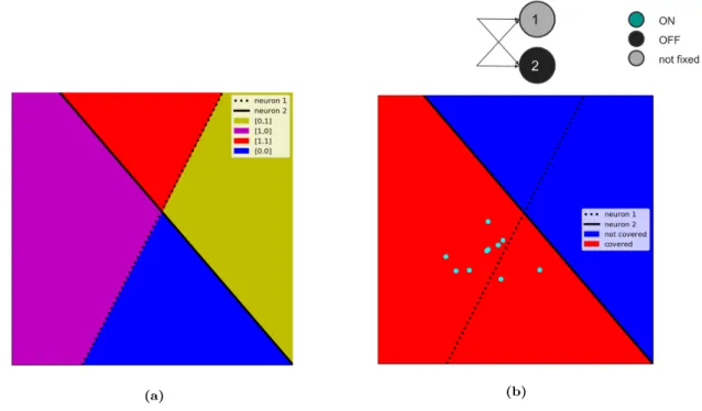
An activation region is a convex subspace of the input space [31], which cor-responds to one unique activation pattern of the network. The network creates a distributed partitioning [4, 48] in its input space by defining a collection of bent hyper-planes [30, 74], where each neuron defines one hyperplane. Subfigures 1.1.a and 1.1.c show input space partitionings over a two dimensional (2D) subspace for two networks with the same number of hidden network parameters1 _{(HNPs). Intuitively, activation}

regions are the connected components [31, 60] between the bent hyperplanes, i.e., the colored regions in the subfigures 1.1.a and 1.1.c.

In the field of neural network expressivity, there is on-going research to estimate the number of activation regions a neural network can create in its input space [30, 60, 63, 65]. Using the tools developed in the network expressivity research, one can view neuron activations inside the network as unions of activation regions in the input space. With this approach the properties of sparse and dense architectures can be compared while leveraging the activations of the networks.

1_{The term} _{hidden network} _{refers to all the layers before the output layer. Hidden network}

pa-rameters are the trainable papa-rameters of the hidden network, i.e., weights and biases of the hidden layers.

(10)

(a) (b)

(c) (d)

Figure 1.1: Two models that have 9472 parameters in their hidden networks have been trained to recognize fashion items with the MNIST Fashion dataset. On the first row there is a dense network with 16 hidden neurons, and on the second row a sparse network with 400 hidden neurons. In the first column both models split a 2D plane in the input space to activation regions. The plane is spun by three images, one from each class 0, 1 and 9. The images are marked with a circle, square, and triangle, respectively. In the second column the networks define minimal blankets w.r.t. class 9. A minimal blanket is a union of activation regions (highlighted red) which activates the subnetwork that is specialized to the phenomenon. The MBH algorithm uses the hypervolume of the minimal blanket to compute the specialization of the network.

(a) A fully parameterized network, density=1.0, with 16 hidden neurons (12,4) splits a 2D plane to 56 regions.

(b) The dense network does not specialize to recognize the class 9, but defines atrivial blanket, which covers the whole input space.

(c) A sparse network, density≈0.034, with 400 hidden neurons (LeNet 300,100) splits the same 2D plane to 34 909 regions.

(11)

5 Leveraging the connection between APs and ARs is not enough to make FFNNs interpretable by itself. Using activation regions to analyze FFNNs is problematic, since the computational requirements to precisely construct an input space partitioning are intense: the exact input space partitioning for a network with 22 hidden neurons can take over 30h to compute [74].

In this work I explain the successes of random and optimized sparsity by

analyzing the distributed partitionings that networks create in their input spaces. My approach is compatible with the existing explanations, and in addition it offers an intuitive explanation why networks with random sparsity perform better than dense networks with the same number of hidden network parameters.

A sparse model defines more hyperplanes in the input space than a dense model with the same number of HNPs, because each neuron defines exactly one (bent) hy-perplane in the input space. Defining more hyhy-perplanes enables the model to split the input space to more (activation) regions [87]. In Figure 1.1 the sparse network splits the 2D plane to over 500 times more activation regions than the dense network, regardless of both having the same number of HNPs.

Defining more regions has been associated with the network’s ability to approx-imate a more complex function [30, 60, 63, 65, 66, 74], and therefore sparse networks can approximate more complex functions than dense networks with the same num-ber of HNPs. As seen in figures 3.4 and 3.5, models that define more hyperplanes (sparse) perform better than models that define less hyperplanes (dense). In other words, quantity over quality with hyperplanes.

While defining more hyperplanes enables the model to approximate more complex functions, it is not the only potential benefit from distributing parameters over larger number of neurons. As discussed earlier, the ability to learn concepts on different levels of abstraction is the core of the deep learning paradigm. My thesis is that having larger number of neurons enables the network to specialize to the features in the data more distinctly.

As my main contribution, I define network specialization, accompanied by a specialization measure to evaluate it, and an algorithm to compute it. Network specialization is a novel concept, which considers how distinctly a feed forward neural network has learned to recognize high level features in the data. Intuitively, if a feed forward networkF is specialized to recognize images (image domain) or singing (audio domain) of a certain species of birds, then it has a subnetworkS that is activated only

by samples (image or audio) that represent the bird species it is specialized to.

(12)

the specialization measure for a FFNN. It uses the network’s decision patterns1 _to

identify the subspace, which the network associates with a given high level feature. The algorithm uses a greedy heuristic to find the smallest subnetwork, which is activated by inputs with the high level feature. The computationally prohibitive con-struction of the full input space partitioning is avoided by computing the partitioning on a lower dimensional subspace. This way the partitioning is computed precisely, which guarantees that no activation region in that subspace goes unnoticed. By aver-aging over randomly chosen subspaces, and using the same subspaces to measure the specialization of different networks, the MBH algorithm approximates the full input space partitioning in reasonable time, regardless of the exponential time complexity of the problem.

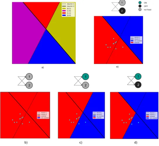
In subfigures 1.1.b and 1.1.d, a 2D plane in the input space is split into regions by two networks with the same number of HNPs. The color of region indicates if it belongs to the subspace which the network associates with the high level feature: red regions are associated, blue regions are not.

Because MBH evaluates the distributed partitioning in the input space, which is shared between the networks that solve the same problem, it can be used to compare networks with any number of hidden layers of arbitrary width. It is also training agnostic, meaning that it does not need to be present during the training of the network, but can be applied to any trained network.

With MBH one can numerically evaluate the specialization of any FFNN, in any domain. Only a dataset with labeled high level features is needed: for example, in datasets designed for supervised learning, some high level features have been labeled as classes. The dataset can be different from the training or validation data used to train the model, which enables evaluating how specialized the model is w.r.t. any concept that can be embodied in the data.

While network specialization can in part explain why sparse networks perform so well, it can also make the networks more interpretable. MBH provides a tool to evaluate how tightly a FFNN outlines any user defined abstract concept in the input space; an insight that directly communicates how well the network expresses the core concept of deep learning.

I test my hypotheses by comparing sparse and dense models in two scenarios: 1) sparse and dense models with the same number of HNPs, and 2) sparse and dense models that have the same architecture2. In the first scenario the sparse networks are

1_{A decision pattern is a part of the full activation pattern of the network; it specifies the activation}

statuses of some subset of neurons [26].

2_{When comparing different FFNNs, by "architecture" I refer to the number of neurons and how}

(13)

7 pruned at random, and therefore the effort of initializing a sparse network is compara-ble to the dense counterparts. In the second scenario sparse networks have optimized sparsity, which compensates for the loss of trainable parameters compared to the dense (fully parameterized) models. For example, comparing the "lucky" subnetworks (win-ning tickets in the LTH [18]) to the fully parameterized, dense networks fall under the second scenario.

The scope of this work is limited to the image domain, and piecewise linear feed forward neural networks with ReLU activation function. Because of the limited space of this work, I evaluate models on MNIST Digit and Fashion datasets, leaving the more comprehensive evaluation for future work. It is good to note that even though this work mainly considers the image domain, network specialization can be applied to any domain where architectures include feed forward networks.

To summarize, the contributions presented in this work are

• Network specialization, a new concept that considers how distinctly the hid-den network of a FFNN has learned to recognize some abstract, user defined concept (sections 4.1 and 4.2, Definition 4.5).

• Specialization measure to evaluate, how specialized a FFNN is (Section 4.3,

Definition 4.7).

• MBH algorithm to compute the specialization measure in a reasonable time,

regardless of the exponential time complexity of the problem (Chapter 5, Algo-rithm 1).

• Intuitive explanation for the performance of sparse networksby viewing

neural networks as collections of bent hyperplanes (Section 3.3). This includes the ability to approximate more complex functions (Subsection 3.3.1), and to specialize more, both evaluated with experiments in the image domain (Chapter 6).

To build the background for network specialization, I will start by reviewing existing literature and defining relevant concepts. In Chapter 2, I will cover sparsity, and in Chapter 3 activations in artificial neural networks. In Chapter 4, I will introduce network specialization, and in the following Chapter 5 I propose MBH algorithm to measure it. The algorithm will then be used in the experiments of Chapter 6 to evaluate my hypothesis that sparse networks specialize more to high level features than dense networks with the same number of hidden network parameters.

number of non-pruned weights, but the same number of neurons, distributed to layers in the same way.

(14)

(15)

2. Sparsity in Artificial Neural

Networks

Deep neural networks are powerful models with often tens of millions of parameters [5, 20, 46], which causes the models to have a big memory footprint and single inferences that require a billion memory accesses and arithmetic operations [91]. These resource requirements are often prohibitive, especially when the models are used in edge devices such as mobile platforms, wearable devices, or smart health devices [54, 91]. Sparsity has been offered as an answer to these problems over the past decade, while the concept of pruning network weights for better generalization and quicker training dates back to the end of 1980’s [50].

A sparse neural network has some of its parameters removed, or otherwise made inactive [20]. A sparse network with some fixed architectureAhas therefore less (active) weights than a dense network with the same architecture. Sparsity of a neural network means the following in this work:

Definition 2.1. Sparsity

LetF be a feed forward neural network withllayers. Each layer has a weight matrixWl to store the weight parameters of that layer. The networkF issparse, if a significant2

number of the entries in the weight matrices are zeroes.

The opposite of a sparse network is a dense network. In a dense network an evident majority of the entries in the weight matrices are non-zero. If a FFNNF has only non-zero parameters, then its density d= 1. If 90% of the trainable parameters3

are removed or set to zero, then the density of F is d= 0.1.

A network can be incentivized to be sparse by adding L1 or L2 norm of the

weights to the loss function [29], which is called L1 or L2 regularization, respectively.

Another way to introduce sparsity is dropout [34], where some randomly chosen entries

2_{There is no absolute measure when a matrix is sparse. In the context of neural networks, removing}

100 entries from a 300×100 matrix (density≈0.997) would not make the matrix sparse. Removing 100 entries from a 20×10 matrix (density 0.5) would be considered a sparse matrix.

3_{In the case of FFNNs trainable parameters are the weights and biases of the network.}

(16)

are treated as zeroes during each forward pass during the training of the network. In this work, however, I will concentrate on sparsity achieved by pruning. Pruning a network means removing or otherwise disabling entries from the weight matrices of the network.

While there has been several successes in reducing the memory footprint and computational requirements of dense models, while maintaining comparable accuracy [29, 54, 73, 91], the field is under constant development. It is far from clear how the networks should be pruned, and what is important for the performance of a sparse network [19, 20, 52].

In this chapter, I will introduce important concepts related to network sparsity, and take a more detailed look at the Lottery Ticket Hypothesis: a conjecture on the existence of trainable sub-networks in dense, overparameterized networks [18]. I begin by defining some core concepts related to ANNs in Section 2.1. In Section 2.2, I define and explain network pruning as means to obtain sparse neural networks. I conclude by bringing together the benefits of optimized sparsity in Section 2.3.

2.1 Preliminaries

In this section I define the core concepts related to artificial neural networks (ANNs) that are essential preliminaries for the rest of this work.

ANNs [24] are connected collections of computational units called neurons that are usually organized in layers. For the purpose of this work, a neuron can be defined as follows:

Definition 2.2. Neuron [24, 31]

Let ni be a neuron that computes a scalar output yi,

yi =g(ai) (2.1) ai =fa(xi;wi, bi) = dl X j=0 xijwij +bi, (2.2)

where dl is the input dimension of the neuron, ai ∈R is a pre-activation that is a dot product between the input vector xi ∈ Rdl and neuron’s weight vector wi ∈ Rdl plus the bias term bi ∈R, and g(·) is an activation function.

For the network to learn a non-linear input distribution, the activation function

g(·) needs to be non-linear [24]. In this work, I will concentrate on networks that have rectified linear unit (ReLU) as their activation function, formally g(x) = max(0, x) [27].

(17)

2.1. Preliminaries 11 In the case of ReLU, the non-linearity results from the different treatment of negative and positive values. When x _> 0 the pre-activation stays unaffected;

g(a) =a ⇐⇒ a_>0. If the pre-activation is negative, however, the value is rectified to 0; g(a) = 0 ⇐⇒ a <0.

In this work, I mainly consider traditional feed forward neural networks (FFNN), which feed the input through the network one layer at the time using the output of one layer as the input of the next layer. The feed forward layer can be defined as

Definition 2.3. Feed Forward Layerfollowing [60]

Let n be a set of k neurons, which all have the input dimension of d0. Together the

neurons form a feed forward layer fl(·), which maps its input x to an output y by applying all of the layer’s neurons to the input and then concatenating the neurons’ outputs to a vector

y=fl(x) = [g(fa(x;w1, b1), g(fa(x;w2, b2), . . . , g(fa(x;wk, bk) ], (2.3) where x∈ _Rd0_, _y∈

Rk, and g and fa are as defined in equations 2.1 and 2.2, respec-tively.

As seen in Equation 2.3, all the neurons in a feed forward layer share the same input x, but each neuron applies linear transformation to the input with their own weights and biases. The linear transformations are passed through the activation func-tion g(·), and those outputs concatenated as the output of the layer.

When several feed forward layers are stacked on top of each other, so that one layer’s output is another’s input, the construction is called a feed forward neural net-work. Following [60]:

Definition 2.4. Feed Forward Neural Networkfollowing [60]

is a composition ofl feed forward layers. It defines a function F :_Rd0 −→

Rm, whered0

is the dimension of the input space andm is the dimension of the output space. The functionF is of form:

F(x; Θ) =fout◦fl◦fl−1◦ · · · ◦f1(x), (2.4)

where each layer maps its input xl to an output yl. Input xl is the output of the previous layer xl = yl−1 for all layers other than the input layer, for which it is the

input of the network.

The last layer of the network is known as the output layer. A FFNN can be divided to two parts: the output layer, and all other layers before it. Since the user only observes the output layer of the network to know the output of the network, the layers preceding the output layer are also known as the hidden layers of the network.

(18)

It is important to note that the layer which outputs the class or regression decision of the network never accesses the input data directly. The signal and the noise in the data are processed by the hidden layers, with the intention to extract the signal that is important for the decision of the output layer. Therefore the hidden layers, also known as thehidden network1, can be seen as a feature extractor that prepares the input data for the output layer.

If the activation functiong is linear, then the network will collapse to a single lin-ear function, and it does not llin-earn non-linlin-ear phenomena [24]. When using a non-linlin-ear activation function, however, even the simple feed forward architecture can approxi-mate complex, non-linear functions to an arbitrary precision: feed forward networks can approximate any Lebesgue integrable function, and are therefore universal function approximators [36].

An example of a function that one might be interested to approximate could be classifying if a patient has cancer or not, based on their medical records. In this example the input space is the medical record, where each entry is a value of one input dimension, e.g. 70kg could be the value of a dimension "weight of the patient". The output space could be one dimensional: a floating point number representing the probability that the patient has cancer. Because of the universal approximation theorem, it is certain that if the function that reliably maps a medical record to cancer diagnose exists, there exists FFNN that approximates it precisely.

Neural networks do not necessarily approximate any interesting function at the initialization of the network. The parameters of the network (weights and biases of Equation 2.2 in the case of FFNNs) are drawn from some distribution when the network is initialized. It is highly unlikely to draw parameters that would right away approxi-mate some function the user is interested in approximating. Therefore the initialized parameters have to be changed for the network to approximate the target function.

Changing the values of the parameters of the network is called training the net-work. Data that represents the behaviour of the target function, gradient based meth-ods, and the back propagation algorithm are used to train the network to approximate the target function better [24]. Even though the universal approximation theorem says that there exists a set of parameters with which a sufficiently large network can approximate any target function, it does not say that the optimal parameters can be found.

How to train and optimize neural networks to approximate the target function is the core question in neural network research [24]. One aspect of it is the architecture of the networks: some architectures are better suited to learn to approximate a given target function than others. For example, some problems are easier to approximate

(19)

2.2. Pruning 13 with deep architectures, where the network is constructed from many narrow layers instead of few wide layers. This approach is also known as deep learning, which has provided good results in several problem domains [48].

FFNNs have been known to be universal function approximators for more than 30 years. Recently it has been shown that depth-bounded [47] and width-bounded [53] rectified networks1 are universal approximators as well. Since ReLUs were applied to stabilize the training of deep neural networks in 2011 [22], ReLUs have become widely used in deep learning [31, 44, 47, 74, 80].

2.2 Pruning

Pruning means removing a network’s weights, usually by setting them to zero [20]. Traditionally in machine learning, a model which has more parameters is expected to be more powerful, i.e. is able learn more complex target functions. However, there is a growing body of work [11, 12, 14, 16, 18, 28, 29, 38, 51, 52, 54, 57, 61, 68, 71, 73, 82, 83, 86, 90] showing that this expectation does not hold true on pruned neural networks: removing trainable parameters (weights) of the networks does not significantly hurt the models’ performance, and in some cases makes the networks to perform better than the original, unpruned models.

There are several strategies for which weights ought to be pruned and when. Sim-ply put, one can prune weights either before, during, or after training. Corresponding pruning strategies are pre-defined sparsity [14], iterative pruning [18], and traditional pruning [29], respectively.

Another aspect to tell pruning strategies apart is to consider wether weights are pruned in a structured [54, 83] or unstructured [29, 91] manner. The former prunes collections of weights, such as whole filters or convolutions in a CNN; the latter means pruning weights individually, without paying attention to any bigger structures of weights.

A third choice to make regarding pruning is which weights are pruned, i.e. define the pruning criteria. Magnitude pruning is the most common choice [20], although other strategies have been proposed as well [85, 90]. The weights can be pruned without sophisticated pruning criteria, in which case the weights are pruned at random [14]. In the context of this work,random sparsityrefers to networks that are pruned at random, and optimized sparsity to networks that have been pruned with a more sophisticated pruning criteria.

The fourth aspect of pruning to consider is the finality of a pruning decision: can

1_{Rectified network uses solely ReLUs as its activation function. All the networks examined in this}

(20)

a once pruned connection be revived later in the pruning process? When the network topology is also optimized, i.e. pruned weights can be "revived" throughout the training process, pruning is dynamic pruning ordynamic sparsity [16, 17, 29, 71].

The four different aspects of pruning weights of a neural network are presented in Table 2.1.

Aspect of Pruning Approaches

Timing Before / During / After training Granularity Structured / Unstructured

Criteria Optimized / Random

Finality Pruned weights can / cannot be revived later in the process

Table 2.1: A simple framework for classifying neural network pruning strategies regarding the timing, granularity, pruning criteria, and finality of the pruning.

In the later chapters of this work, I will concentrate on examining networks that are randomly pruned prior to the training. Benefits that follow from sparsity obtained in this manner can be credited to the sparsity itself, and not other aspects of the pruning method.

Before proceeding to study the inherent benefits of sparsity in neural networks in the following chapters, I will examine a phenomenon related to optimized sparsity.

2.2.1 The Lottery Ticket Hypothesis

Recently Frankle and Carbin conjectured that large, overparameterized FFNNs con-tain subnetworks, which have won the initialization lottery [18]. They argued that the existence of "lucky initializations" (winning tickets, WTs) would explain why the training of a large network converges successfully with a higher probability than the training of a smaller network. The large, overparameterized network contains many subnetworks, "lottery tickets", making it more probable that at least one of them is a winning ticket which trains well.

When trained in isolation, these winning tickets perform better than randomly initialized networks that have the same sparsity, i.e. normal lottery tickets. Winning tickets can be trained to the same test accuracy as the original dense network, regardless of WTs having potentially less than 10% of the parameters of the dense network.

The hypothesis, as presented in the original work, is stated as follows:

Conjecture 2.1. The Lottery Ticket Hypothesis [18]

(21)

2.3. Pruning Can Be Training 15

such that—when trained in isolation—it can match the test accuracy of the original network after training for at most the same number of iterations.

The default method to to obtain winning tickets (WTs) goes as follows:

1. Initialize a dense, overparameterized network.

2. Train the dense network until it converges.

3. Prune the network to some sparsitys. This is the structure of the winning ticket.

4. Take the pruning mask from 3 and return weights to their initial values from 1. This is the winning ticket.

Furthermore, the winning tickets are usually found through iterative magnitude prun-ing (IMP) because iterative prunprun-ing produces better sparse networks [18, 29]. It is good to note, however, that the conjecture does not require this, since it doesn’t state anything about the pruning technique used to find these "well" initialized subnetworks. The lottery ticket hypothesis (LTH) has gained a lot of attention during 2019 and 2020 [11, 16, 19, 52, 55, 57, 61, 68, 71, 79, 80, 82, 86, 90]. For the purpose of this work it is interesting for two reasons. Firstly, the existence of winning tickets (i.e. well performing subnetworks) is interesting in itself, since it means that potentially all dense networks could be pruned for a better efficiency and performance. Secondly, the results in the literature are in some parts contradictory, so clearly there remains work to be done on the topic.

There is contradicting evidence on the role of winning tickets. Most of the cri-tique is directed towards the role of winning tickets: for some datasets and optimization schemes winning tickets "do not exist", or are not distinguishable from random initial-izations after substantial amount of training [20, 52]. This implies that winning tickets do not play a central role in the trainability of large neural networks, unlike the authors of the conjecture originally hypothesized.

2.3 Pruning Can Be Training

The contemporary approach to teach a network to approximate a function, i.e. to solve a problem, is to change the learnable parameters of the network with gradient based methods. The goal is to find a good set of parameters which solve the problem. However, fine-tuning the network’s parameters is not the only way to teach the network to approximate some function.

Pruning the network’s weights can be training [90]. In fact, a sufficiently large piece-wise linear network can be pruned to approximate any (Lebesgue integrable)

(22)

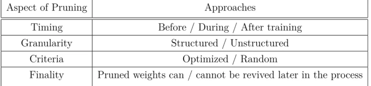
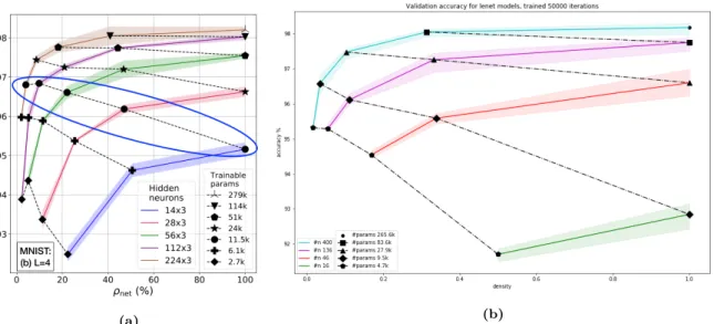
function without changing the unpruned weights at all [55]. This contributes to the success of sparse networks with optimized sparsity: a successful pruning might teach the network to solve the problem without training the weights. This can be seen in Figure 2.1, as well as in [90].

Figure 2.1: Neural networks can be taught to solve a problem without changing the weights. Vali-dation accuracy of Lenets with (300,100) hidden neurons on Digit MNIST, averaged over 5 models. Intervals are min and max. Blue and yellow have untrained parameters. Blue (winning tickets) are obtained from the fully parameterized models (black) as described below Conjecture 2.1. In short, the WTs have the pruning mask obtained from the trained fully parameterized models, but the weights are from the initialized state, before the training. The pruning is done with the one-shot magnitude pruning. Yellow has random pruning and re-initialized parameters. Red marks the trained winning tickets that is, red is blue after training. Green is yellow after training. The x-axis is density.

As explained in the Chapter 3, the weights of a neuron define the orientation of the hyperplane it spans in the input space. Both removing some of the weights and changing the values of the weights through training alter the orientation of that hyperplane. Therefore it is not surprising that, by removing some of the weights, the hyperplane can be adjusted into a favourable position for the purpose of solving the problem at hand.

In Figure 2.1 a vastly overparameterized network (300 + 100 = 400 hidden neu-rons) can achieve consistently over 80% validation accuracy on a simple image classi-fication problem without training the weights, just removing 70-75% of them. Figure 2.1 also demonstrates the Occam’s hill [67] produced by pruning: by removing too few or too many weights (left and right edges of the plot), the network does not achieve a high validation accuracy. By removing enough, but not too many, of the weights the hyperplanes are adjusted enough to (partially) solve the problem without changing the

(23)

2.3. Pruning Can Be Training 17 values of the weights at all.

Both the winning tickets (blue) and randomly pruned, re-initialized networks (yel-low) in Figure 2.1 reach rather similar validation accuracy (red and green, respectively). This supports the view presented in [20, 52] that randomly pruned, freshly initialized networks can be trained to the same validation accuracy as the winning tickets. Strong conclusions cannot be drawn, however, since winning tickets found with one-shot mag-nitude pruning are reported to be significantly worse, than ones found with iterative magnitude pruning [18, 90].

Training the network by removing weights is not the only benefit of a well chosen pruning mask. Removing connections can serve as a way to reduce the noise without disturbing the signal, enabling the model to exploit the redundancy in the data [14].

2.3.1 Exploiting Redundancy in the Data

Sometimes the data have dimensions which do not hold any information about the phenomena that the user is modelling, i.e. the dimensions are redundant. In the case of hand written MNIST digits this is clearly visible. The pixels at the borders of the images do not tell anything about the digit in the image because the digits are centralized and do not reach the edges of the image. Since those dimensions (pixels near edges) do not have any information about the phenomena (hand written digits) that is being modelled, they only introduce noise to the input of the network. Removing the connections to these dimensions improves the signal to noise -ratio of the input that the network receives.

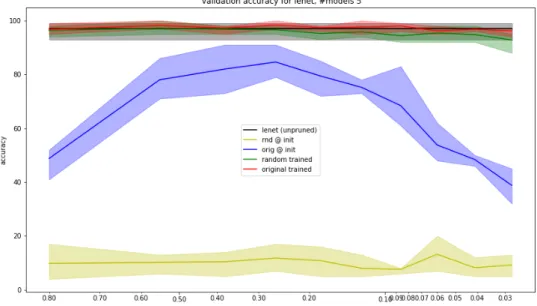
Stochastic gradient descent (SGD) does this naturally, without any further incen-tivising1_{. In Figure 2.2 the right-hand column shows learned pruning masks obtained}

with one-shot magnitude pruning (OSMP). The more weights are pruned, the more dimensions near the border of the images are left completely without connections. This means that after training with the SGD, weights to those uninformative dimensions are so small that they get pruned by the OSMP, and the more informative connections are left for the model to be processed. In other words, pruning a network with a suitable pruning criteria can serve as a feature selector.

If the data are highly redundant, i.e. there are a lot of uninformative or repetitive dimensions, then pruning can improve the quality of the data received by the network by removing connections to these uninformative dimensions. Sparse architectures have been successful especially in tasks with highly redundant data, discussed for example in [14]. This suggests that one factor contributing to the success of winning tickets is the

1_{In this experiment scenario with Digit MNIST.}

(24)

ability to prune noise from the input signal, rather than having a "lucky initialization", like the authors of LTH originally argued [18].

(a)

(b)

Figure 2.2: Heatmaps of active connections on the input layer of Lenet (300,100 -hidden neurons) after pruning. A white pixel indicates, that every neuron in the input layer has unpruned connection to that dimension; a black pixel means that all the connections have been pruned. Each heatmap is the sum of five networks. In (a) the density of the pruned networks is 0.552, in (b) the density is 0.028. Left: random sparsity. Right: optimized sparsity (OSMP).

(25)

3. Activations in Piecewise Linear

Neural Networks

When a neural network processes data, some of its neurons are activated by the input. Different inputs activate different neurons, and some neurons are more often active than others. The study of activations in neural networks examines the activation statuses of the neurons to understand the networks and their behaviour better.

Over the past 6 years there has been an increasing interest towards activations in neural networks to answer questions on expressivity [60, 66] and interpretability [26, 44] of FFNNs. I will extend on the tools developed on this field in Chapter 4 to define and measure the specialization of FFNNs.

In this chapter, I define and explain key concepts related to activations in artificial neural networks (Section 3.1), and review how activations are used in the existing literature (Section 3.2). Finally, in Section 3.3, I argue why sparse networks can be expected to specialize more than dense networks with the same number of HNPs.

3.1 Background and Definitions

In this section, I cover essentials on activations inside a network (Subsection 3.1.1) and activations in the input space (Subsection 3.1.2). Before proceeding to the activations, I will briefly define piecewise linear (PWL) networks.

A piecewise linear function consists of several linear functions which apply to collection intervals of real numbers [74]. For example, the ReLU -function2 _{is a PWL}

function that consists of two linear functions defined for intervalsx <0 andx_>0, x∈

R.

If a feed forward neural network uses ReLU as its activation function, the function that the network expresses is a piecewise linear function [22]. Intuitively this means that the network defines a different linear function for each linear region of the input space, and the location of an input x in the input space will determine which linear

2_{See Section 2.1 for details on ReLU.}

(26)

function will be applied to x, when processed by the network.

A piecewise linear network is a neural network, whose activation functions are piecewise linear. Therefore a rectified network is a PWL network. I am restricting my analysis to piecewise linear networks because the existing research on network activations concentrates solely on PWL networks.

3.1.1 Activations in a Neural Network

The atomic unit which can have an activation status in a FFNN is a neuron. ReLUs offer an intuitive example for defining when a neuron is active. Since the negative pre-activation ai results a constant 0 with ReLU, I shall say that a neuron is inactive (or "off") when the pre-activation is negative, and active (or "on") otherwise. In more general terms:

Definition 3.1. Neuron activation status, following [60, 65]

A neuron’s activation status changes, when the activation function g has irregular be-haviour, such as an inflection point or non-linearity. The number of different activation states of a neuron α = rg + 1, where rg is the number of irregular behaviours of the activation function.

The set of possible activation statusesa depends on the activation function. For example, for a neuron with ReLU activation, aReLU ={0,1} and αReLU = 2. For hard hyperbolic tangent (hard tanh), atanh ={−1,0,1}and αtanh = 3 [65].

We can also consider the activation status of the whole network, i.e. the activation statuses of all neurons simultaneously. The activation status of a network can be expressed as an activation pattern:

Definition 3.2. Activation pattern A [31, 65]

Let F be a neural network with k neurons, g the activation function of the network, and a the set of possible activation statuses of g. An activation pattern for F is an assignment to each neuron an activation status [31]:

A:={az, z is a neuron in F} ∈ak. (3.1) Let x be an input and Θ the set of parameters of F. Let AP(·) be a function that maps F, Θ, and x to the corresponding activation pattern A [65], that is,

A =AP(F(x; Θ) ) . (3.2) As seen in the Equation 3.2, the activation pattern of the network depends both on the input x and the parameters of the network Θ. Changing either of them can change the resulting pattern A.

(27)

3.1. Background and Definitions 21 Because the size of an activation pattern depends on the architecture of the network F, and a different set of parameters Θ can result in a different activation pattern, for the sake of readability we will assume the architecture1 _of _F _{and Θ fixed,}

if not stated otherwise.

When a neuron’s activation status is fixed, the neuron has an activation con-straint. In an activation pattern, all neurons have an activation constraint. In some applications this is too restrictive, as one might be interested in the behaviour of some particular subset of neurons.

The more fine grained patterns, which consider only a subset of neurons, are calleddecision patterns:

Definition 3.3. Decision Pattern σ [26]

Let F be an FFNN, x an input of F, and A an activation pattern of F when F

processes x. A decision pattern σ is a sub-pattern of A. That is, σ specifies the activation statuses for some subset of neurons inF, when F processes x.

When the subset of neurons coincide with a layer of the network, the decision pattern can be called alayer pattern.

Definition 3.4. Layer Pattern L, following [26]

LetF be a FFNN, and L the i:th layer of F. A layer pattern Li is a decision pattern

σ, for which all the neurons constrained in σ belong to L, and all neurons in L are constrained in σ.

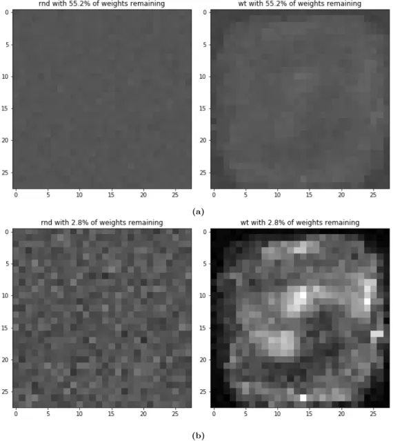
In Figure 3.1 the difference between activation, decision, and layer patterns is illustrated with a simple example.

Decision patterns, and therefore layer patterns as well, outline a subnetwork of the FFNN. A subnetwork S is a subset of neurons, which is defined by a decision pattern σ, and it is connected to the input space through neurons that feed into σ. Formally,

Definition 3.5. Subnetwork S

LetF be a FFNN, andσ a decision pattern of F. The subnetworkS, whichσ defines, consists of the neurons that 1) belong toσ, or 2) feed into the neurons in σ.

If a neuron’s output affects the input of another, the former feeds into the latter [26]. If a FFNN is fully connected, then every neuron on a layerl feeds into all neurons on the layerl+ 1. This also extends deeper into the network: if a neuronn1 on layer 1

feeds into the neuronn2 on layer 2, andn2 feeds into the neuronn3 on layer 3, thenn1

feeds into n3. For the purpose of feeding, a FFNN is considered as an directed acyclic

graph (DAG).

(28)

Figure 3.1: Illustration of (a) an activation pattern, (b) a decision pattern, and (c) a layer pattern of a sparse FFNN with (4,4,2) neurons and ReLU as its activation function. Gray nodes do not have an activation constraint, black nodes are required to be inactive and green nodes active, when the networks processes an input. Note that in an implemented version of decision and layer patterns the neuron indices should be saved alongside the activation statuses.

For example, the decision pattern presented in Subfigure 3.1.b defines a subnet-work of seven neurons: all four neurons form the first layer, and the three constrained neurons from the second layer.

A subnetwork is activated by an input x, when the processing ofx results in the same decision pattern which defines the subnetwork. If a subnetwork S of a FFNN F

is defined by a decision pattern σ, then all the neurons constrained in σ should have the same activation status when F processes x, for S to be active.

The activations inside the neural network can be used to improve the inter-pretability and performance of the networks, as seen later in Subsection 3.2.2. However, the usage of activations is not limited to neurons inside the networks: every activation inside the network can be interpreted as a region in network’s input space.

3.1.2 Activations in the Input Space

A neural network creates a distributed1 partitioning [4, 48] in its input space. Inputs located in different parts of the partitioning result in a different activation pattern

1_{In a}_distributed _{partitioning, a point in the input space is classified by each hyperplane spun by}

the model, e.g. each neuron of a neural network. A model that creates a local partitioning, e.g. a k-means clustering, connects each input to a local region in the input space, rather than making a binary classification with each computational unit [4]. Because of this theknowledge representation learned by a neural network is said to be distributed.

(29)

3.1. Background and Definitions 23 when they are processed by the network1 _{[26, 31, 30].}

As discussed in the beginning of this section, a PWL neural network defines different linear functions for the different parts, or regions, of the partitioning. When moving from one linear region to another in the input space, the linear function changes as one or more of the activation functions g change from one linear state to another. The boundary between two or more linear regions in the input space is ahyperplane.

Definition 3.6. Hyperplane H [60, 63]

Hyperplane Hi is a subspace in the input space:

Hi :={x∈Rd0|fa(x;wi, bi) = 0}. (3.3) It is spun by a neuronni with the weight vectorwi, biasbi, and ReLU as the activation function. The pre-activation function fa is defined in Equation 2.2.

For example, consider a two dimensional input spaced0 = 2 and a neural network

with ReLU activations. Each neuron on the first layer of the network "draws a line" in the input space, and the line is located where the neurons pre-activationai changes its sign. That line is the hyperplane a neuron defines in the input space.

A collection of all hyperplanes of the first layer of the network (one for each neuron) is called ahyperplane arrangement [60, 75]. A hyperplane arrangement consists of linear hyperplanes, i.e. the hyperplanes do not bend.

However, hyperplanes defined by neurons that are deeper in the network can bend. The inputs received by neurons after the input layer have passed through the non-linear activation function g, and therefore the inputs can be defined by different linear functions depending on the interval of the original input.

The set of hyperplanes defined by a neural network with has several layers is referred to as acollection of bent hyperplanes:

Definition 3.7. Collection of Bent Hyperplanes HF [31, 60]

A collection of bent hyperplanes is a set of hyperplanes

HF :={H1, H2, . . . , Hn} in the input space, spun by a network F that has n neurons.

In Figure 3.2 the collection of bent hyperplanes defined by a small DNN is visu-alized to illustrate the bending of hyperplanes.

Each hyperplane splits the input space to two regions: one where the spanning neuron is active, and another where it is not. Since the activation statuses of neurons

1_{This equals to changing the input} _x_{in Equation 3.2, while keeping the networks parameters Θ}

(30)

Figure 3.2: Example of a collection of bent hyperplanes, defined by a FFNN with ReLU activations and three layers with 2 neurons each. The network is the same as in Figure 2 in [74]: it has a 2 dimensional input space, and the outputs of the neurons areha =max{0,−x1+x2},hb=max{0, x1+

x2−4},hc=max{0,−ha−3hb+ 4},hd=max{0,−3ha−hb+ 4},he=max{0, hc+ 3hd−4}, and

hf = max{0,3hc +hd −4}. The image has been created with my implementation of the sweep hyperplane method [30, 31, 62, 75], which is used as a function in the MBH algorithm (Algorithm 1). change only at the hyperplanes, each region between the hyperplanes corresponds to exactly one activation pattern A. Those regions are called activation regions:

Definition 3.8. Activation region R [31]

Let F be a rectified FFNN with k neurons, the parameters Θ, and aReLU = {0,1} the set of possible activation statuses of the neurons of F. The activation region corresponding to an activation pattern A of F, is

R(A; Θ) :={x∈_Rd0_|₍₋₁₎ai_f

a(xi;wi, bi)>0, i∈[0, k]} (3.4) where d0 is the dimension of the inputs space, wi the fixed weights, bi the fixed bias, and ai ∈aReLU the integer representing the activation status of neuron ni.

It is good to note that the definition of an activation region (AR) provided above applies only to rectified networks, as used in the original source [31]. For the equation to be applicable to other PWL activation functions, such as the hard tanh, the term (−1)ai _{should be changed to support the possible activation states of the activation}

function. See Definition 3.1 for how the possible neuron activation statuses depend on the activation function.

(31)

3.1. Background and Definitions 25 Another way to define activation regions is by leveraging the definition of hy-perplanes. If one removes the hyperplanes from the input space, then the connected components remaining are the activation regions.

Definition 3.9. Non-empty Activation Regions[31]

Non-empty activation regions are the connected components of the complement Rd0\ SHF, i.e. a set of points in the input space delimited by the hyperplane ar-rangement HF (possibly open towards infinity).

This definition is widely used [26, 60, 63, 65], although it is mistakenly labeled to definelinear regions instead of activation regions. As pointed out in [31], two adjacent regions separated by a hyperplane could coincidently have the same linear function, in which case together they would form one region in the terms of linear regions.

An important property of activation regions1 _{is their convexity:}

Lemma 3.1. Activation regions are convex polytopes in the input space [31]. Let F be a rectified network. Then for every activation pattern A and any set of parameters Θ of F, each activation region R(A; Θ) is convex.

Intuitively, the convexity of a region means that a closed segment connecting two points, which belong to the region, is always completely inside the region. For example, from 2D shapes all triangles, circles and squares are convex, but a five pointed star is not.

Lemma 3.1 is not restricted to ReLUs but holds for any piecewise linear activation function [31]. In Figure 3.2, each differently colored region is a convex activation region2_.

While individual ARs are guaranteed to be convex, unions of ARs are not. Each individual neurons defines two unions of activation regions in the input space: one where the neuron is active, and another where it is not. These unions of ARs are not necessarily convex.

A neuron with an activation constraint is a decision pattern, and therefore defines a subnetwork. As discussed in the end of Subsection 3.1.1, a subnetwork is active when the processed input results in the same decision pattern which defines the subnetwork. When the activation status of a neuron is fixed, then the part of the input space which causes the neuron to have the same activation status as the constraint, is said to activate the subnetwork defined by the neuron and its activation constraint.

1_{The convexity has been proven already earlier [65], but was said to concern}_linear _{regions instead}

of activation regions.

2_{For an image that showcases the building of activation regions by layers, see for example figure 1}

(32)

(a) (b)

Figure 3.3: A minimal example of a union of activation regions that activate a subnetwork. (a) A neural network with two neurons splits the input space into four activation regions.

(b) The decision pattern {n2: 0} has one activation constraint, and it defines a subnetwork. The

subnetwork is activated by the union of two activation regions colored red in the subfigure (b), where the neuron 2 is off.

The concept of the input space activating a subnetwork is illustrated in Figure 3.3. The network of two neurons can have 8 different subnetworks in total. Four different subnetworks are defined by decision patterns of a single neuron ({n1: 1},

{n1: 0}, {n2: 1}, and {n2: 0}), and another four by subnetworks with two activation

constraints (both neurons on, both neurons off, and another two with the neurons having different activation statuses). The latter four subnetworks correspond to the four activation regions in the figure: the decision patterns defining the subnetworks are actually activation patterns because they define the activation statuses of every neuron in the network.

The subnetworks defined by a single neuron, however, are activated by unions of activation regions. In this simple example all four possible unions defined by a subnetwork are convex, but this is not guaranteed with deeper networks that have more neurons.

A subnetwork is activated by the connected component of the input space, where the subnetwork is active. The other way around, any input that is covered by the subnetwork results in the same activations that define the subnetwork when processed by the network. More formally,

(33)

3.1. Background and Definitions 27

Definition 3.10. Activation of Subnetwork

LetF be a FFNN, and σ a decision pattern that defines a subnetwork S. If an input

x, x∈_Rd0_{, results the decision pattern} _σ _when _x _{is processed by} _F_{, then} _x _activates

S. Here d0 is the dimension of the input space.

When x activates S, it can be noted with S(x) = T rue, and naturally S(x) =

F alsewhen x does not activate S.

The parts of the input space, which activate a subnetwork, always coincide with a union of activation regions:

Lemma 3.2. A subnetwork is activated by a union of activation regions.

Proof. To prove that the set of inputs which activates a subnetwork always co-incides with a union of activation regions, it is sufficient to show that there does not exist an activation region with inputs that activate the subnetworkand inputs that do not.

LetF be a FFNN, which partitions the input space to non-empty activation regions _Rd0_\ S

HF (Definition 3.9). Let σ be a decision pattern, which defines a subnetwork S (Definition 3.5). Let the set of inputs, which activate S, be

x:={x∈ Rd0_| _S₍_x₎_}_.

Now, contrary to the original assumption, I will assume instead that there exists an activation region Rx, which includes both inputs that activate S, and inputs that do not activate S. Let the former set of inputs be xon := {x ∈

Rx| S(x)} and the latter xof f :={x ∈ Rx| ¬S(x)}. Based on Definition 3.10, an input activates a subnetwork if it results in the same decision pattern which defines the subnetwork. Therefore, inputs in xon must result in a different activation patterns than inputs inxof f, when processed byF. However, all inputs inxon and

xof f belong to the same activation regionRx, and based on Definition 3.8 all inputs in the same activation region result the same activation pattern when processed by F. This is a contradiction and therefore there cannot be an activation region

Rx which includes both inputs that activateS and inputs that do not activate S. Therefore the original assumption holds true: x always coincides with a union of activation regions ∀ S.

A union of activation regions that activates a subnetworkScan be called ablanket

defined byS. The blanket covers the part of the input space which activates S.

Definition 3.11. Blanket B

LetF be a FFNN, and σ a decision pattern which defines a subnetwork S of F. The blanketB defined by S is the union of activation regions which activatesS.

(34)

The concepts defined in this section lay the foundation for understanding the pub-lished results and use cases of activations in PWL neural networks (Section 3.2), why sparse architectures benefit from distributing the HNPs to a larger number of neurons (Section 3.3), and how the specialization of a FFNN can be measured (Chapter 4).

3.2 Related Work

In the existing literature, activations of PWL neural networks are used mainly for two purposes: to estimate the expressivity of the different network architectures [30, 31, 59, 60, 63, 65, 66, 74] and to interpret and leverage the decision process of the networks [1, 8, 15, 26, 44, 47, 56, 62, 81]. Chronologically, the former precedes the latter: the ground work on estimating the minimal upper bounds [60] dates to 2014, while papers on verifying the behaviour of PWL networks using the activations [15, 44] were published during 2017.

In this section, I will briefly review how the activations in PWL neural networks are used to 1) assess the networks’ expressivity (Subsection 3.2.1) and to 2) improve their interpretability and performance (Subsection 3.2.2).

3.2.1 Activations as an Expressivity Measure

The expressivity of a neural network refers to the networks capability to express a function. The more expressive a network is, the more complex functions it can approx-imate.

When one considers the expressivity of a network, analyzing only the functions it is capable to approximate is a rather limited way to estimate its expressivity, since the theoretical results may assume networks of infinite width or depth [36, 60]. In addition, the functions approximated in the literature might be arbitrary compared to the real world use cases (see [60]). By estimating the number of linear/activation regions a network creates in the input space, one can compare different architectures with a more concrete measure.

Using Definition 3.2, an activation pattern can be seen as the fingerprint of a neural network’s decision process given some input. Since each activation pattern corresponds to one activation region, counting activation patterns is fundamentally the same thing as counting activation regions. The former are activation states of the network for some input x, and the latter subspaces in the input space_Rd0_.

The number of activation regions has been widely used as an expressivity measure, and across the literature it is agreed without further scrutiny that the more activation regions a network can produce, the more expressive it is [31, 60, 59, 65, 74, 89]. The