by
Javonne Jason Martin
Thesis presented in partial fulfilment of the requirements
for the degree of Master of Science (Computer Science) in
the Faculty of Science at Stellenbosch University
Supervisors: Dr R. S. Kroon
Dr H. A. C. de Villiers
December 2018
The financial assistance of the National Research Foundation (NRF) and the MIH Media Lab towards this research is hereby acknowledged. Opinions expressed and conclusions arrived at, are those of the author and are not necessarily to be attributed to the NRF or MIH Media Lab.
Declaration
By submitting this thesis electronically, I declare that the entirety of the work contained therein is my own, original work, that I am the sole author thereof (save to the extent explicitly otherwise stated), that reproduction and pub-lication thereof by Stellenbosch University will not infringe any third party rights and that I have not previously in its entirety or in part submitted it for obtaining any qualification.
December 2018
Date: . . . .
Copyright c 2018 Stellenbosch University All rights reserved.
Abstract
Creating 3D Models using Reconstruction Techniques
J J MartinThesis: M.Sc (Computer Science) December 2018
Virtual reality models of real world environments have a number of compelling applications, such as preserving the architecture and designs of older build-ings. This process can be achieved by using 3D artists to reconstruct the environment, however this is a long and expensive process. Thus, this thesis investigates various techniques and approaches used in 3D reconstruction of environments using a single RGB-D camera and aims to reconstruct the 3D environment to generate a 3D model. This would allow non-technical users to reconstruct environments and use these models in business and simulations, such as selling real-estate, modifying pre-existing structures for renovation and planning. With the recent improvements in virtual reality technology such as the Oculus Rift and HTC Vive, a user can be immersed into virtual reality environments created from real world structures. A system based on Kinect Fusion is implemented to reconstruct an environment and track the motion of the camera within the environment. The system is designed as a series of self-contained subsystems that allows for each of the subsystems to be modified, expanded upon or easily replaced by alternative methods. The system is made available as an open source C++ project using Nvidia’s CUDA framework to aid reproducibility and provides a platform for future research. The system makes use of the Kinect sensor to capture information about the environment. A coarse-to-fine least squares approach is used to estimate the motion of the camera. In addition, the system employs a frame-to-model approach that uses a view of the estimated reconstruction of the model as the reference frame and the incoming scene data as the target. This minimises the drift with respect to the true trajectory of the camera. The model is built using a volumetric approach, with volumetric information implicitly stored as a truncated signed distance function. The system filters out noise in the raw sensor data by us-ing a bilateral filter. A point cloud is extracted from the volume usus-ing an
ABSTRACT iii
orthogonal ray caster which enables an improved hole-filling approach. This allows the system to extract both the explicit and implicit structure from the volume. The 3D reconstruction is followed by mesh generation based on the point cloud. This is achieved by using an approach related to Delaunay trian-gulation, the ball-pivot algorithm. The resulting system processes frames at 30Hz, enabling real-time point cloud generation, while the mesh generation oc-curs offline. This system is initially tested using Blender to generate synthetic data, followed by a series of real world tests. The synthetic data is used to test the presented system’s motion tracking against the ground truth. While the presented system suffers from the effects of drift over long frame sequences, it is shown to be capable of tracking the motion of the camera. This thesis finds that the ball pivot algorithm can generate the edges and faces for synthetic point clouds, however it performs poorly when using the noisy synthetic and real world data sets. Based on the results obtained it is recommended that the obtained point cloud be preprocessed to remove noise before it is provided to the mesh generation algorithm and an alternative mesh generation technique should be employed that is more robust to noise.
Uittreksel
3D-modelle met behulp van Rekonstruksie Tegnieke
J J MartinTesis: M.Sc (Rekenaar Wetenskap) Desember 2018
Modelle in virtuele realiteit van werklike omgewings het ’n aantal belangrike toepassings, soos byvoorbeeld die behoud van die argitektuur en ontwerpe van geskiedkundig belangrike geboue. 3D kunstenaars kan ingespan word om om-gewings te modelleer, maar dit is ’n lang en duur proses. Hierdie proefskrif ondersoek verskillende tegnieke en benaderings wat gebruik word in die 3D rekonstruksie van omgewings deur gebruik van ’n enkele RGB-D kamera en beoog om die 3D rekonstruksie van die omgewing te omskep in ’n 3D-model. Hierdie sal nie-tegniese gebruikers toelaat om self modelle te skep van omge-wings, en om hierdie modelle te gebruik in besigheid toepassings en simulasies, soos byvoorbeeld die verkoop van vaste eiendom, die wysiging van bestaande strukture vir beplanning en opknapping. Met die onlangse tegnologiese ver-beteringe in die veld van virtuele realiteit soos, byvoorbeeld, die Oculus Rift en HTC Vive, kan ’n gebruiker geplaas word in ’n virtuele omgewing wat ge-skep was vanaf strukture in die werklike wˆereld. ’n Stelsel gebaseer op Kinect Fusion word ge¨ımplementeer om ’n omgewing te rekonstrueer en die beweging van die kamera binne die omgewing te volg. Die stelsel is ontwerp as ’n reeks selfstandige modules wat die afsonderlike aanpassing, uitbreiding of vervanging van die modules vergemaklik. Die stelsel word beskikbaar gestel as ’n open source C++ projek met behulp van Nvidia se CUDA raamwerk om reprodu-seerbaarheid te bevorder en bied ook ’n platform vir toekomstige navorsing. Die stelsel maak gebruik van die Kinect-sensor om inligting oor die omgewing vas te vang. ’n Grof-tot-fyn kleinste kwadraat benadering word gebruik om die beweging van die kamera te skat. Daarbenewens gebruik die stelsel ’n beeld-tot-model benadering wat gebruik maak van die beraamde rekonstruk-sie van die model as die verwysingsraamwerk en die inkomende toneel data as die teiken. Dit verminder die drywing ten opsigte van die ware trajek van die kamera. Die model word gebou met behulp van ’n volumetriese benadering,
UITTREKSEL v
met volumetriese inligting wat implisiet gestoor word as ’n verkorte getekende afstandfunksie. Die stelsel filter ruis in die ruwe sensor data uit deur om ’n bilaterale filter te gebruik. ’n Puntwolk word uit die volume onttrek deur ’n or-togonale straalvolger te gebruik wat die vul van gate in die model verbeter. Dit laat die stelsel toe om die eksplisiete en implisiete struktuur van die volume te onttrek. Die 3D-rekonstruksie word gevolg deur maasgenerasie gebaseer op die puntwolk. Dit word behaal deur ’n benadering wat verband hou met Delaunay triangulasie, die bal wentelings algoritme, te gebruik. Die resulterende stel-sel verwerk beelde teen 30Hz, wat intydse-puntwolkgenerasie moontlik maak, terwyl die maasgenerering aflyn plassvind. Hierdie stelsel word aanvanklik ge-toets deur om met Blender sintetiese data te genereer, gevolg deur ’n reeks werklike wˆereldtoetse. Die sintetiese data word gebruik om die stelsel se afge-skatte trajek teenoor die korrekte trajek te vergelyk. Terwyl die stelsel ly aan die effekte van wegdrywing oor langdurige intreevideos, word dit getoon dat die stelsel wel die lokale beweging van die kamera kan volg. Hierdie proefskrif bevind dat die bal wentelingsalgoritme die oppervlaktes en bygaande rande vir sintetiese puntwolke kan genereer, maar dit is sterk gevoelig vir ruis in sintetiese en werklike datastelle. Op grond van die resultate wat verkry word, word aanbeveel dat die verkrygde puntwolk vooraf verwerk word om ruis te verwyder voordat dit aan die maasgenereringsalgoritme verskaf word, en ’n alternatiewe maasgenereringstegniek moet gebruik word wat meer robuust is ten opsigte van ruis.
Contents
Declaration i Abstract ii Uittreksel iv Contents vi List of Figures ixList of Tables xiv
1 Introduction 1
1.1 Problem Statement . . . 2
1.1.1 Aims and Objectives . . . 2
1.2 Contributions . . . 3
1.3 Outline . . . 4
2 Background 5 2.1 Pinhole Camera Model . . . 5
2.1.1 Converting to Camera Space . . . 5
2.1.2 Converting to World Space . . . 8
2.2 Transformation Matrix . . . 8
2.2.1 Homogeneous Coordinates . . . 9
2.2.2 Rotation Matrix . . . 10
2.2.3 Building the Transformation Matrix . . . 11
2.2.4 Quaternions . . . 13
2.3 Least Squares . . . 15
2.3.1 Linear Least Squares . . . 16
2.3.2 Non-Linear Least Squares . . . 17
2.4 3D Modelling . . . 17
2.4.1 Polygon Modelling . . . 19
2.4.2 Curve Modelling . . . 19
2.4.3 Sculpting . . . 19
CONTENTS vii
2.4.4 Manifold Mesh . . . 20
2.5 Kinect Sensor . . . 21
2.5.1 Generating the World . . . 22
2.6 Summary . . . 23
3 Related Work 24 3.1 Motion Estimation . . . 24
3.2 SLAM Solutions . . . 27
3.2.1 Extended Kalman Filter . . . 28
3.2.2 Rao-Blackwellized Particle Filter . . . 29
3.2.3 GraphSLAM . . . 30
3.3 Alternative Solutions . . . 31
3.3.1 Bundle Adjustments . . . 32
3.3.2 Kinect Fusion . . . 32
3.3.3 Parallel Tracking and Mapping . . . 33
3.3.4 Dense Tracking and Mapping . . . 34
3.3.5 Benchmarks . . . 34
3.4 Depth Estimation . . . 34
3.5 Mesh Reconstruction . . . 35
3.5.1 Mesh reconstruction techniques . . . 36
3.5.2 Mesh Reconstruction Benchmarks . . . 40
3.6 Summary . . . 40 4 Methodology 43 4.1 Reconstruction . . . 43 4.2 Mesh Generation . . . 44 4.3 Evaluation . . . 44 4.3.1 Reconstruction . . . 45 4.3.2 Mesh Generation . . . 46 4.4 Summary . . . 46 5 Kinect Fusion 47 5.1 System Overview . . . 47 5.2 Pyramid Construction . . . 48 5.3 Bilateral Filter . . . 48
5.4 Iterative Closest Point . . . 51
5.4.1 Projective Data Association . . . 52
5.4.2 Error Function . . . 52
5.4.3 Solving the Non-Linear System . . . 53
5.4.4 Iterative Closest Point Algorithm . . . 55
5.5 Truncated Signed Distance Function . . . 56
5.5.1 Signed Distance Function . . . 58
CONTENTS viii
5.6 Raycasting . . . 66
5.7 Point Cloud Extraction and Hole Filling . . . 69
5.8 Summary . . . 71
6 Mesh Reconstruction 72 6.1 Overview . . . 72
6.2 Pivoting Algorithm . . . 73
6.2.1 Finding a Valid Seed Triangle . . . 76
6.2.2 Pivoting Operation . . . 79
6.2.3 Join and Glue Operation . . . 79
6.2.4 Multiple Passes . . . 85
6.3 Summary . . . 86
7 Experiments 88 7.1 Data sets . . . 88
7.1.1 Synthetic Data Sets . . . 89
7.1.2 Real-world Data Sets . . . 92
7.2 Trajectory Analysis . . . 95 7.2.1 Translation Test . . . 96 7.2.2 Rotation Test . . . 100 7.2.3 Circling Table . . . 103 7.2.4 Moving Around . . . 106 7.2.5 Additional Experiments . . . 113 7.2.6 Conclusion . . . 113
7.3 Point Cloud Analysis . . . 114
7.3.1 Hole-Filling . . . 114
7.3.2 Point Cloud Analysis of Synthetic Data Sets . . . 119
7.3.3 Point Cloud Analysis of Real-World Data Sets . . . 125
7.3.4 Summary . . . 131
7.4 Mesh Generation . . . 132
7.4.1 Synthetic Data Sets . . . 132
7.4.2 Experiments . . . 133
7.5 Summary . . . 137
8 Conclusion 140 8.1 Summary . . . 140
8.1.1 Aims and Objectives . . . 140
8.2 Future Work . . . 143
8.3 Reproducibility . . . 143
List of Figures
2.1 Illustration of the basic pinhole camera model. . . 6
2.2 Illustration of a ray of light from an object falling on the image plane for the X and Y axes. . . 6
2.3 Illustration of a ray of light from an object falling on the image plane for the Y and Z axes. . . 7
2.4 Illustration of the shifted image plane into the positive XY plane. 7 2.5 Illustration of a rotation around a fixed point. . . 12
2.6 Illustration of gimbal lock. . . 14
2.7 A cube displaying the normals to the surface in teal. Normals indicate the exterior direction that surface is facing. This helps the modelling application know the inside and outside of the model. 18 2.8 Illustration of polygon modelling concepts. . . 18
2.9 Illustration of a curve with two control points. . . 19
2.10 Illustration of sculpting a sphere. . . 20
2.11 Illustration of a few non-manifold meshes. . . 21
2.12 Illustration of the two versions of the Microsoft Kinect. . . 22
2.13 Example of Kinect output. . . 22
3.1 Illustration of the graph created during GraphSLAM. . . 31
3.2 Illustrates the construction of triangles using Delaunay triangu-lation on a set of 3D points projected on a 2D plane. . . 37
3.3 Illustrates a configuration of the marching cube intersection that generates a line in 2D. . . 40
LIST OF FIGURES x
4.1 An illustration of the proposed system and its different subcom-ponents. The system takes input in the form of a depth image and an RGB image. The depth image passes through the bilateral filter and propagates to the TSDF component. The RGB image is inserted directly into the TSDF component where the results are fused. The ICP component uses the input from the bilateral filter and the ray caster to compute the best motion estimate for the system. The TSDF component uses the motion estimate from the ICP component to fuse the depth image with the RGB image from the correct position. Following this, the ray caster generates a virtual image to provide the ICP component with a new model view. The ray caster also extracts points from the TSDF volume
when points move out of the mapping area. . . 45
5.1 An outline of the original Kinect Fusion system. . . 48
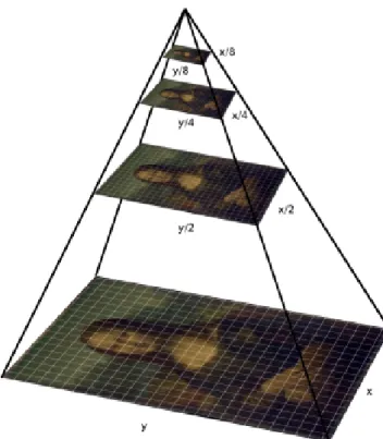
5.2 Illustrates the image pyramid with the successive sub-sampled images. . . 49
5.3 Illustration of a point being back projected on a different image plane. . . 53
5.4 Illustrates the point-to-plane error metric between two surfaces. 53 5.5 Illustrates the ground truth and line of sight of the depth camera. 59 5.6 Illustrates the TSDF values around the surface. . . 60
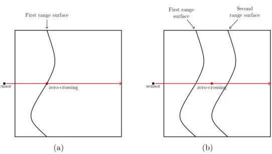
5.7 Illustrates the zero-crossing before and after integrating a second measurement. . . 61
5.8 Illustration of limiting the update region of the TSDF values. . . 62
5.9 Illustration of the TSDF volume being virtually translated. . . . 64
5.10 Illustrates the camera moving outside the threshold region and the TSDF volume being virtually translated. . . 65
5.11 Illustrates the rays being cast from the virtual camera into the TSDF volume. . . 68
5.12 Illustration of the different points found between the two ray cast-ing techniques. . . 70
6.1 Illustration of the BPA in 2D. . . 73
6.2 Illustration of the pivoting operation in R3. . . 74
6.3 Illustration of the BPA in 2D using a slightly larger ball. . . 75
6.4 Illustration of multiple fronts with the ball unable to pivot be-tween them. . . 76
6.5 Illustration of a ball pivoting to a point with the incorrect normal direction. . . 78
6.6 Illustration of a sphere generated in the outward half-space of the points. . . 78
LIST OF FIGURES xi
6.8 Illustration of the Joinoperation on an unused point. . . 81
6.9 Illustration of the Joinoperation in the second situation, a used point that is an internal point. . . 81
6.10 Illustration of the Join operation in the third situation, a used point that is on a front. . . 82
6.11 Illustration of the Joinoperation creating coincident edges. . . . 82
6.12 Illustration of the different types of Glueoperations. . . 83
6.13 Illustrates the consecutive loop of theGlue operation. . . 83
6.14 Illustration of the closed loop from the Glueoperation. . . 84
6.15 Illustration of the two fronts merging in 3D. . . 84
6.16 Illustrates the split loop of the Glue operation. . . 85
6.17 Illustrates a merge loop from the Glue operation. . . 86
7.1 Illustration of the Table TopScene. . . 89
7.2 Illustration of the RoomScene. . . 89
7.3 Illustration of the global coordinate system in Blender. . . 91
7.4 Illustration of frames from the Rotation Test data set. . . 92
7.5 Illustration frames from the Circling Table data set. . . 93
7.6 Overview of the Room Closed Loopdata set. . . 94
7.7 Frames from the Deskdata set. . . 94
7.8 Overview of the Lab Roomdata set. . . 95
7.9 The results of the translation error and the rotation error for each axis. . . 97
7.10 The results for the estimated position of the camera for each axis during the Translation Test. . . 98
7.11 The results for the absolute rotation of the camera for each axis during the Translation Test. . . 99
7.12 The dot product between the ground truth quaternion and esti-mated quaternion for the Translation Test. . . 100
7.13 The results for the translation and rotational error for theRotation Test data set. . . 101
7.14 The dot product between the ground truth’s quaternion and es-timated quaternion for the Rotation Test. . . 103
7.15 The results for the absolute rotation of the camera for each axis during the Rotation Test. . . 104
7.16 The results for the position of the camera for each axis during the Rotation Test. . . 105
7.17 The results for the error in the translation and rotation during the Circling Table data set. . . 107
7.18 The results for the absolute position of the camera for each axis during the Circling Table data set. . . 108
7.19 The results for the absolute rotation of the camera for each axis during the Circling Table data set. . . 109
LIST OF FIGURES xii
7.20 The results for the error in the translation and rotation during
the Moving Around data set. . . 110
7.21 The results for the absolute position of the camera for each axis during the Moving Around data set. . . 111
7.22 The results for the absolute rotation of the camera for each axis during the Moving Around data set. . . 112
7.23 Illustration of the data used to test the different point cloud ex-traction techniques. . . 114
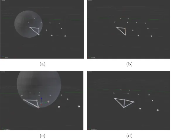
7.24 Illustration of the extracted point cloud using the original ray casting technique. . . 115
7.25 Illustration of the extracted point cloud using the orthogonal ray casting technique. . . 116
7.26 Illustration of the experiment setup to demonstrate interference that can occur while integrating range images into the TSDF volume. . . 116
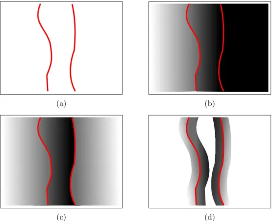
7.27 Illustration of the TSDF values when the depth images are inte-grated. . . 117
7.28 Illustration of the extracted point cloud using the orthogonal ray caster and limiting the voxel update region. . . 118
7.29 Illustration of the hole filling properties when limiting the update region. . . 118
7.30 The results of the three variations of ray casting. . . 119
7.31 Illustration of the point cloud generated from theCircling Table data set. . . 120
7.32 Illustration of the point cloud generated from theMoving Around data set. . . 122
7.33 Illustrates a side by side comparison of the original model view with a view from the extracted point cloud for theMoving Around data set. . . 123
7.34 Illustrates the global axis in Blender for theMoving Arounddata set. . . 124
7.35 Illustration of the extracted point cloud from the Room Closed Loop data set. . . 125
7.36 Illustration of the visible warping of the scene due to the drift. . 126
7.37 Illustration of the RGB-D data taken from the Kinect. . . 127
7.38 Illustration of incorrectly reported depth data. . . 127
7.39 Illustration of noise generated from interfering IR light. . . 128
7.40 Illustration of the reflectivity of IR light. . . 128
7.41 Illustration of the artefacts generated from sensor noise. . . 129
7.42 Illustration of noise from the depth image. . . 130
7.43 Illustration of the extracted point cloud from the Lab Roomdata set. . . 130
LIST OF FIGURES xiii
7.45 Illustration of the Terrain reconstructiondata set. . . 133 7.46 Illustration of theTerrain reconstructiondata set reconstructed
into a mesh. . . 134 7.47 Illustration of the mesh reconstructed from the Stanford Bunny
data set. . . 134 7.48 Illustration of the generated mesh from the extracted point cloud
of the Circling Table data set. . . 135 7.49 More illustrations of the generated mesh from the extracted point
cloud of the Circling Table data set. . . 136 7.50 Illustration of the reconstruction using the extracted point cloud
from the Moving Around data set. . . 137 7.51 Illustration of the reconstruction using the extracted point cloud
List of Tables
7.1 Properties of the data sets with scenes used and the area that the camera moves through. . . 89 7.2 Average error over all frames for the Translation Testdata set. 96 7.3 The magnitude of the error averaged over all frames of each
trans-lation and rotation component for the Rotation Test data set. 103
List of Algorithms
1 Pseudocode for the Kinect Fusion’s ICP algorithm. . . 57 2 Pseudocode for the AddEquation function of the ICP algorithm. 58 3 Pseudocode for the ray casting operation. . . 69 4 Pseudocode for the ball-pivoting algorithm. . . 77
List of Common Symbols
d The distance represented by the TSDF volume.
dj A destination point in the local coordinate system used in the ICP algo-rithm.
dgj A destination point in the global coordinate system used in the ICP algo-rithm.
f The focal length for the X and Y axis, the distance between the camera centre and the image plane.
fx The focal length for the X axis.
fy The focal length for the Y axis.
gmax The maximum value that the distance function can be.
gmin The minimum value that the distance function can be.
gs A vector that contains the dimensions of the volume containing the voxels.
G(x) The combination of a series of signed distance functions with x repre-senting a point in 3D space.
g(x) The signed distance function withx representing a point in 3D space.
I The image plane (as illustrated in Figures 2.2, 2.3 and 2.4).
Ii An RGB-D image captured at time i.
Pi Point cloud generated from the RGB-D image at timei.
K The camera intrinsic matrix. Converts between 3D world coordinates to 2D camera coordinates.
Nld,g The destination normal map constructed from the pyramid at level l in the global coordinate system.
ndj The normal vector at the destination point in the local coordinate system.
List of Common Symbols xvii
nd,gj The normal vector at the destination point in the global coordinate sys-tem.
ns
j The normal vector at the source point in the local coordinate system.
ns,gj The normal vector at the source point in the global coordinate system.
Ns
l The source normal map constructed from the pyramid at levell.
Nls,g The source normal map constructed from the pyramid at level l in the global coordinate system.
o The centre of the image plane.
ox The displacement of the optical axis along the X axis.
oy The displacement of the optical axis along the Y axis.
pcamera The position of the camera in 3D space.
pH A homogeneous coordinate in 2D space.
pobject The position of a object in 3D space.
R The raw depth image obtained from the Kinect sensor.
RayDir The unit vector of RayNext. The direction of the ray being cast from the camera’s position to the image plane.
RayNext This is a vector generated from a ray being cast from the camera’s position to a pixel location on the image plane.
sj A source point in the local coordinate system used in the ICP algorithm.
sgj A source point in the global coordinate system used in the ICP algorithm.
StepSize The size that the ray is incrementally increased in length by.
ti+1 The translation vector obtained from the transformation matrix Ti+1. u A pixel location on the image plane.
ˆ
u A back projected pixel location.
ux The X pixel coordinate of an image.
uy The Y pixel coordinate of an image.
List of Common Symbols xviii
vcs A vector that contains the size in meters that each voxel represents for each axis.
Vld,g The vertex map of the destination points created from a pyramid levell
in the global coordinate system.
Vs
l The vertex map of the source points created from a pyramid level l.
Vls,g The vertex map of the source points created from a pyramid level l in the global coordinate system.
Chapter 1
Introduction
Low cost 3D-sensing hardware such as the Microsoft Kinect have facilitated broad-based development of faster and higher quality 3D reconstruction. As a result, many advances have been made in the field. Research on structure from motion (SFM), multi-view stereo (MVS) and improving hardware have led to more efficient systems. SFM is a ranging technique for estimating 3D structures from 2D images. MVS is a group of techniques that uses stereo correspondence to reconstruct objects in 3D. With the emergence of low cost virtual reality equipment, such as the Oculus Rift and the HTC Vive, 3D reconstructions could be used in game engines to display environments in vir-tual reality. Currently there are many proposed solutions to the problems of 3D reconstruction and mesh reconstruction. This thesis aims to investigate the problem of 3D reconstruction and mesh reconstruction for the creation of virtual reality environments.
Most 3D reconstruction techniques are either used in research for self driv-ing cars or commercial robotics systems that mainly focus on trajectory re-construction. It is difficult for a non-technical user to make use of these 3D modelling techniques. The proposed system opens its usages to many appli-cations such as creating assets from real world objects in gaming, viewing 3D models of properties online and simulations for virtual reality exposure therapy.
Virtual reality exposure therapy is a treatment method where patients are slowly exposed to traumatic stimuli with the assistance of virtual reality equipment. This allows patients to interact with their phobia virtually, without access to the real phobia itself. The use of this system could allow technicians to assist therapists in simulating real-world environments for patients.
Such a system could also be applied in the property industry. Instead of viewing buildings by visiting them, the model could be placed on a website to display the 3D mesh of the building for potential clients to view. This would allow measurements of the rooms and dimensions to be easily accessible for the potential clients.
CHAPTER 1. INTRODUCTION 2
1.1
Problem Statement
Virtual environments are used to create visualizations for simulations, virtual reality and games. These environments are time-consuming to create, requiring artists to model and texture the environment. Creating a digital version of a room automatically from photos could accelerate the process and reduce the cost of modelling.
This could be performed by ‘scanning’ the environment through taking photos and collecting the depth information. This would allow automatic reconstruction of the environment from this data. This approach would reduce the time taken to model the environment and would not require the skill of a CGI artist. The process of ‘scanning’ requires the use of a depth sensor such as the Cyberware 3030 (Cyberware Incorporated, 2018) or Microsoft Kinect (Microsoft, 2018). The ability to reconstruct a room gives a person the power to create a digital version of an environment by pre-arranging a room according to their desire.
One key problem is the scarcity of open-source integration of existing tech-niques.
The 3D reconstruction problem has several challenges that must be over-come. Two things are required to reconstruct the environment: the position of the camera and the view from that position. The main challenge in 3D reconstruction is computing the position of the view.
Mesh reconstruction has the problem of ambiguity when generating meshes from point clouds. Since information about the surface is not known, mesh reconstruction algorithms need to determine the surface given a set of arbitrary points.
1.1.1
Aims and Objectives
The aim of this work is to create a system that allows a non-technical user to build a 3D model relatively quickly and export it to a common format that can be easily incorporated into 3D modelling tools and virtual reality simulations. In order to do this, the following objectives were set out for the system proposed in this thesis.
• Collect depth and colour data from the environment.
• Estimate the motion of the depth sensor.
• Achieve online motion estimation speeds.
• Pre-process the sensor data to reduce noise.
CHAPTER 1. INTRODUCTION 3
• Enable generation of large scale environments.
• Extract the implicit and explicit structure of the environment as a point cloud.
• Generate a mesh from the final point cloud data.
• Integrate colour data into the mesh.
• Export the meshed point cloud with the texture map in a universal format.
1.2
Contributions
This thesis makes the following contributions:
• A system was developed that allows for 3D reconstruction of environ-ments. A scan-matching algorithm was implemented to estimate the motion of the camera. This works in conjunction with a volumetric model to reduce drift using a frame-to-model scan-matching technique. The volumetric model was assisted by a ray caster that allows the system to extract the implicit structure of the environment.
• A plug-in was developed that allowed synthetic data sets to be created along with ground truth information. This was achieved using Blender’s Python interface.1
• Provision was made for large scale environments by using a volumetric approach to 3D reconstruction in combination with a wrap-around in-dexing system that allows the system to continuously map new areas (Section 5.5.2).
• It is demonstrated in Section 7.4 that the ball-pivoting algorithm (Bernar-dini, Mittleman, Rushmeier, Silva and Taubin, 1999) is more suited for object reconstruction, as opposed to being used for environment recon-struction.
• To facilitate reproducibility and future work by other researchers, the entire system is provided as an open-source implementation under the MIT license (Martin, 2017).
1Scripts are provided in an open-source repository to create synthetic data sets and record the ground truth trajectory (https://gitlab.com/pleased/3d-reconstruction).
CHAPTER 1. INTRODUCTION 4
1.3
Outline
This thesis is divided into 8 chapters. Chapter 2 (Background) introduces the concepts and the mathematical methods that are required to understand the rest of the thesis. Chapter 3 (Related Work) reviews existing techniques that are used for 3D reconstruction and mesh generation. Chapter 4 (Methodology) specifies the techniques that will be used in the system to achieve the aims and objectives of this thesis. Chapter 5 (Kinect Fusion) details the implementation used to reconstruct the point cloud as mentioned in the methodology. Chap-ter 6 (Mesh Generation) discusses generating a mesh from the point cloud obtained in the Kinect Fusion chapter. Chapter 7 (Experiments) describes the experiments performed to test the system’s performance and analyses the results. This is followed by a summary of the system’s performance. Chapter 8 (Conclusion) summarizes the thesis results and considers the proposed sys-tem’s advantages and disadvantages. Finally, the chapter discusses additional work that could be considered for improving on reported results.
Chapter 2
Background
This chapter provides essential background information about various tech-niques and mathematical methods used in this thesis. This chapter covers the pinhole camera model (Section 2.1), which facilitates conversions between camera coordinates and real-world coordinates. 3D transformation matrices (Section 2.2) and quaternions (Section 2.2.4) are also discussed, providing a means for representing the location and orientation of the camera. Next, linear and non-linear least squares optimisation is presented to provide a method to compute motion estimates for the 3D transformation (Section 2.3). This is fol-lowed by the foundations of 3D modelling, demonstrating various techniques used during the 3D modelling process (Section 2.4). Finally, some background information about the Kinect sensor is provided (Section 2.5).
2.1
Pinhole Camera Model
The pinhole camera model describes a method for projecting the three-dimensional world onto a two-dimensional image plane. Imagine a closed box with a very small aperture that allows light in. Rays of light from an object in front of the box pass through the aperture and fall on the interior surface at the rear of the box. These light rays that pass through the aperture create an inverted image on this surface. This is illustrated in Figure 2.1.
2.1.1
Converting to Camera Space
The pinhole camera projection process is described mathematically as follows: Given a 3D Cartesian coordinate system, a point pcamera (representing the pinhole) located at the origin, a 2D plane I representing the image plane (i.e. the back of the box) with I intersecting the Z axis at pcamera, the point o representing the centre of the image plane, a 3D point pobject, and f the focal length (the perpendicular distance between o and pcamera). In this situation
CHAPTER 2. BACKGROUND 6
Figure 2.1: The basic pinhole camera model illustrates the reflected light from a tree entering the box through the aperture and falling on the interior surface at the rear of the box.
the Z axis is the optical axis, the direction the camera is facing. The goal is to project the 3D point pobject onto the 2D plane I. Projecting all the objects in the scene in this manner produces an image.
The projection is performed by drawing a line frompobject passing through
pcamera to the plane I. This produces two similar triangles that can be used to compute the projected point on the image plane as shown in Figure 2.2. This process is repeated for the YZ plane in Figure 2.3 producing Equation 2.1 that computes the location on the image plane.
Z X pcamera pobject I Ipobject f −ux z x o
Figure 2.2: This figure demonstrates a ray of light frompobject passing through
pcamera and intercepting the plane I at location −ux. This is illustrated for the XZ axis. (ux, uy) = −f x z , −f y z (2.1)
CHAPTER 2. BACKGROUND 7 Z Y pcamera pobject I Ipobject f −uy z y o
Figure 2.3: This figure demonstrates a ray of light frompobject passing through
pcamera and intercepting the plane I at location −uy. This is illustrated for the YZ axis.
The image plane currently has its centre located at the origin o on the X and Y axes. However, the image centre region does not always coincide with a rectangle centred at the origin in I due to inaccuracies in the camera mount created during the camera’s construction (i.e due to inaccuracies when placing the lens relative to the image sensor), thus ox and oy are introduced to model the displacement of the optical axis. Typically, ox and oy are half the resolution of the image and is added to Equation 2.1 to ensure that the image plane is only defined in the positive XY axis as shown in Figure 2.4. This allows the image coordinates to start at position (0, 0), which is convenient for implementation. This updates Equation 2.1 to produce Equation 2.2.
Z X pcamera pobject I Ipobject f ux z x o
Figure 2.4: This demonstrates a ray of light frompobject passing throughpcamera and intercepting the plane I with the plane shifted such that all intercepts are defined in the positive XY plane.
CHAPTER 2. BACKGROUND 8 (ux, uy) = f x z +ox, f y z +oy (2.2) This produces the coordinates on the image planeI for the objectpobject. For simplicity a matrix K, the camera intrinsic matrix, is constructed that allows this transformation to be applied through matrix multiplication as shown in Equation 2.3. In reality, the focal lengthf is two valuesfx andfy on a low-cost image sensor because each individual pixel (light sensor) on the image plane is rectangular rather than square. The actual value of the focal length, fx, is the product of the physical focal length and the width of the light sensor. Similarly,
fy is the product of the physical focal length and height of the light sensor. The values for the physical focal length, the width of the light sensor and the height of the light sensor can generally not be obtained without physically opening the camera and directly measuring these values. The parameters fx,
fy, ox and oy can be obtained through camera calibration.
K = fx 0 ox 0 fy oy 0 0 1 ux uy 1 = K x y z z (2.3)
2.1.2
Converting to World Space
Given the camera space projection (a 2D image) of the three-dimensional world, it is possible to compute the world space coordinates. The world space coordinates are the 3D positions relative to the origin on the camera. This is done by applying the inverse operations starting with the image space coor-dinates ux and uy to obtain two world coordinates. Since many points in the three-dimensional world can project to the same image location, z is used as the last world coordinate. This is achieved by performing the inverse transfor-mation from the previous section.
K−1 ux uy 1 zworld = x y z (2.4)
2.2
Transformation Matrix
A transformation matrix is a combination of a rotation matrix and a trans-lation vector. An n-dimensional rotation matrix R is an n ×n matrix that comprises the rotational information of the local coordinate system. The ele-ments contained in the rotation matrix are further described in Section 2.2.2. The size of this matrix depends on whether it is a 2D or 3D problem, using
CHAPTER 2. BACKGROUND 9
a 2×2 or 3×3 rotation matrix. The translation vector T is an-dimensional vector, depending on the dimensionality of the problem, containing the x, y
and z translation. The 3D transformation matrix is constructed as follows:
R T 0 1 (2.5)
The transformation matrix is used to translate and rotate points in space. It is also used to convert between different coordinate systems.
2.2.1
Homogeneous Coordinates
Homogeneous coordinates are a way of representing points that allow for affine and projective transformations to be easily represented in the form of a matrix. A point p in R2 is represented by two values such as the points in two coor-dinates. This is extended by adding an extra dimension to the vector p. The new representation is defined as the vector pH with an additional dimension containing the value 1:
p = x y pH = x y 1 (2.6)
To represent an arbitrary point in R2 as a homogeneous coordinate, pH is constructed as shown in Equation 2.7. The variable s is a non-zero scaling factor for the vector. Scaling a homogeneous vector by a non-zero factor does not change the point.
pH = sx sy s (2.7)
To compute the x and y values of a R2 homogeneous vector, one simply divides the vector by the scaling factor as shown
pH = sx sy s = sx/s sy/s s/s = x y 1 (2.8)
Vectors pH1 and pH2 illustrate two vectors that represent the same point.
pH1 = 8 12 4 pH2 = 4 6 2 = 1 2p H1 (2.9)
CHAPTER 2. BACKGROUND 10
Homogeneous coordinates can be extended toR3, which therefore require the use of a vector in R4.
pH3 = sx sy sz s (2.10)
For more information about homogeneous coordinates, the reader is referred to Hartley and Zisserman (2004).
2.2.2
Rotation Matrix
A rotation matrix is a way of rotating points in 2D or 3D Euclidean space. Given a 2D coordinate system, a point p can be rotated around the origin by an angle of φ radians in a counterclockwise direction to produce a new point
q as shown: q=Rp qx qy = cos(φ) −sin(φ) sin(φ) cos(φ) px py (2.11) This concept can be extended to 3D, producing three rotation matrices, one for each axis. Using the parameters θ, φ and α which represent the rotation in radians in the X axis, Y axis and Z axis respectively the following matrices are obtained. Rx(θ) = 1 0 0 0 cos(θ) −sin(θ) 0 sin(θ) cos(θ) (2.12) Ry(φ) = cos(φ) 0 sin(φ) 0 1 0 −sin(φ) 0 cos(φ) (2.13) Rz(α) = cos(α) −sin(α) 0 sin(α) cos(α) 0 0 0 1 (2.14)
These rotation matrices can be consolidated into a single rotation matrix to produce the desired effect of the combined rotations.
CHAPTER 2. BACKGROUND 11
Any rotation matrix R is an orthogonal matrix, therefore the following property holds: the inverse matrix can be computed as follows.
R−1 =RT
It follows that the determinant of the rotation matrix is det(R) = ±1.
We can now use the combined rotation matrix Rzyx to rotate a point p around the origin as follows.
p0 =Rzyxp (2.16)
Similarly the point can be rotated in the opposite direction by computing the inverse rotation matrix or transpose R−1
zyx = RTzyx. This is called the inverse rotation.
RTzyxp0 =p (2.17) Equation 2.16 allows one to transform points around the origin. This will not work for rotating points around a fixed point.
To rotate the point p1 around the fixed pointpF,p1 needs to be adjusted
by subtracting the fixed point pF from the pointp1 as follows
pOrigin1 =p1−pF. (2.18) The point pOrigin1 can now be rotated using the rotation matrix R to obtain the new point pOrigin10
pOrigin10 =RpOrigin1 . (2.19)
When the point has been rotated, it can be adjusted by adding the point
pF to produce the final point p10. The rotation around a fixed point can be
rewritten as shown in Equation 2.20. This is demonstrated in Figure 2.5.
p10 =R(p1−pF) +pF (2.20)
2.2.3
Building the Transformation Matrix
In order to rotate a point p about the origin and then translate it, a rotation matrix R and translation vectorT can be applied as follows:
CHAPTER 2. BACKGROUND 12
pF
p1
(0.5,0.5)
(1,0.5)
(a) Original points
pOrigin1 pO
(0,0) (0.5,0)
(b) Adjusted pointp1 to obtain pOrigin1
pOrigin10 pO (0,0) (−0.35,0.35)
(c) The rotated point pOrigin10 after a
ro-tation by 34π.
p10
pF (0.5,0.5) (0.15,0.85)
(d) p10 The final position of p1 after a
rotation by 34π.
Figure 2.5: This figure illustrates how a rotation around a fixed point is per-formed. Subfigure (a) illustrates the scenario, the point p1 is the point that
needs to be rotated around the fixed point pF. Subfigure (b) illustrates that each point has been moved to the origin by subtracting pF. This results in a new point pOrigin1 . Subfigure (c) illustrates the rotation applied to pOrigin1
resulting in the point pOrigin10 . Subfigure (d) illustrates the points shifted by pF resulting in a rotation of the pointp1 around the fixed point pF producing the point p10.
CHAPTER 2. BACKGROUND 13
This is called a rigid body transformation. The inverse of this transformation can be computed by applying the inverted operations on a point p0 to obtain
RT(p0−T) = RTp0 −RTT=p. (2.22) Equation 2.21 can be condensed by constructing a 4×4 transformation ma-trix M that will apply the rotation matrix R followed by the addition of the translation vector T M = R T 0 0 0 1 . (2.23)
Given this transformation matrix M and a point p in homogeneous coordi-nates, the point can be transformed as follows
p0 =Mp. (2.24)
Similarly, the original point p can be computed given the point p0 and an associated transformation matrix M by multiplying by M−1 to obtain
M−1p0 =p. (2.25) The inverse transformation matrix M−1 exists, and can be obtained from the components of the transformation matrix as
M−1 = RT −RTT 0 0 0 1 . (2.26)
2.2.4
Quaternions
Another method of representing rotations is using quaternions (Hamilton, 1844). Quaternions are a way of representing rotations using only four values. Quaternions were created to get around the problem of gimbal lock when using Euler angles. Gimbal lock occurs when a series of rotations cause a loss of one degree of freedom in three-dimensions. This happens when two of the three axes are in a parallel configuration which cause a rotation around two of the axes to have the same effect, as shown in Figure 2.6. Quaternions approach the rotation from a different perspective. Quaternions use a vector to represent the rotation and can be easily converted to a rotation matrix and back. In computer graphics and the gaming industry, OpenGL uses rotation and trans-formation matrices during rendering. However, when computing rotations,
CHAPTER 2. BACKGROUND 14
(a) (b)
Figure 2.6: Subfigure (a) illustrates a plane with its associated rotation axes. Subfigure (b) shows a configuration such that two gimbals are in alignment, causing gimbal lock.
developers tend to use quaternions when constructing the rotations that need to be applied to the game world. Once this quaternion is constructed, it is converted to its rotation matrix representation and applied to the objects in the scene. Quaternions are an extension of the complex numbers by defining two more values j and k; then the quaternions are
q =w+xi+yj+zk.
with the following properties
i2 =j2 =k2 =−1 (2.27)
ij =k jk =i ik=j. (2.28) To understand how quaternions can be used to represent rotation,qis rewritten as follows
q= (w,v) (2.29)
v= (x, y, z). (2.30)
Represented in this way, quaternions encapsulate the idea that there is a vec-tor vthat represents an axis in space around which the object will be rotated. Given an axis around which the rotation will be performed, the angle of rota-tion is required. The quaternions are always represented as a unit quaternion, i.e. the length of the quaternion is 1. The vector q is further adjusted to encode the rotational angle about the axis as follows
q= (cosθ,(sinθ)v). (2.31) This allows us to store the angle of rotation in the quaternion representation, which can easily be extracted by computing cos−1w. The advantage of using
CHAPTER 2. BACKGROUND 15
quaternions is that quaternion multiplication can combine a series of rotations to produce a single axis around which the rotation occurs. This is the com-bination of all the quaternion rotations. Quaternions also have the advantage of never suffering from gimbal lock, which is a problem when employing Euler angles in rotation. The quaternion is represented as a vector, which allows us to check the similarity of two quaternions by computing their dot product.
2.3
Least Squares
The method of least squares (Stewart, 2007) is a technique used to obtain an approximate solution to an overdetermined system of equations that has no exact solution. It is based on observation values and the values predicted by a candidate solution (expected/ estimated value) minimising the sum of the squared differences between observed value and the estimated value for each of the equations in the system. A residual is such a difference between an actual value and an estimated value. One common purpose of using the least squares method is to fit a data model to a set of observations. An example of this is to fit a collection of (x, y) points to a straight line, y=Dx+C, by determining the coefficients D and C that will minimise the sum of the squared residuals. For example given three points (0, 6), (1, 0) and (2, 0), a straight line needs to be fit to these points. Using the straight line equation the following equations are generated
0·D+C = 6 (2.32)
1·D+C = 0 (2.33)
2·D+C = 0. (2.34) This system has no solution. This is rewritten in the form of
Ax=b (2.35) 0 1 1 1 2 1 D C = 6 0 0 (2.36)
The aim is now to find some D and C that best satisfies this system of equa-tions. The basic idea of solving this is minimising S, the sum of the squared residual functions. The residual function r is the difference between the ob-served valuesyi and the estimated values of the approximationf(xi, x), where
CHAPTER 2. BACKGROUND 16
in the example above.
ri =yi−f(xi, x) (2.37) S = n X i=0 r2i (2.38)
Least squares problems are often divided into two categories: linear and non-linear least squares problems. The difference between non-linear and non-non-linear depends on the parameters that need to be determined. Linear least squares problems use models that are linear with respect to the model parameters. For example solving v and w in
y=vx2+wx+ 2.
However, for example, the following equations are non-linear with respect to the parameters (v, w, σ, µ): y= sinvcosx, y= v σ√2π exp − (x−µ)2 2σ2 +w, ory=w2x+vx.
These equations cannot be solved using linear least squares. An approach to tackling these types of equations will be briefly explained in Section 2.3.2.
2.3.1
Linear Least Squares
Minimising Equation 2.38 can be performed by setting the gradient of S to 0 as follows
∇S = 0. (2.39)
In the linear case, solving Equation 2.39 generates a set of normal equations
ATAx=ATb, (2.40) with corresponding solution
x= (ATA)−1ATb.
Solving Equation 2.40 is equivalent to solving the Equation 2.39. For more information refer to Strang (2016) on least squares. The solutions to computing a linear least squares problem and a non-linear least squares problem diverge before Equation 2.40.
CHAPTER 2. BACKGROUND 17
2.3.2
Non-Linear Least Squares
Solving non-linear least squares problems requires more steps. This is due to the derivative of S in Equation 2.38. The gradient produces a function that does not generally have a closed-form solution. Since the derivative is non-linear, the solution has to be calculated iteratively with an initial estimate x0
for x chosen. At each iteration, an incremental difference that the estimate needs to be updated by will be computed. Given the estimate of the solution
xj at iteration j + 1 and the newly calculated incremental change ∆xj+1, the
estimate at iteration j + 1 is calculated as
xj+1 =xj+ ∆xj+1. (2.41)
Since the derivative is non-linear at each iteration, the model is linearised using a Taylor series expansion around xj. In terms of the linearised model, the gradient is now a list of gradient equations ∂ri
∂x =−J
j
i. At every iteration
xj the Jacobian Jj has to be recalculated due to the changing linearisation point used. Using the Jacobian, each iteration of the non-linear least squares solution is approximated as follows
JTJ∆xj+1 =JT∆b . (2.42) Solving non-linear least squares problems requires multiple iterations and de-pending on the initial value used, the technique can produce a value that is only locally optimal. In the linear case, Equation 2.42 has a constant Jacobian so just one step is needed.
2.4
3D Modelling
3D modelling is the process of developing surface representations of 3D objects. A surface consists of a group of faces. In 3D modelling, there are 3 concepts that are used to create a model: a vertex, an edge and a face. A vertex is a point in R3 defined by an x,yand z coordinate. Two connected vertices form an edge. Three or more coplanar edges in a cycle form a face. Creating these vertices, edges and faces produces a 3D model that can be used in a variety of ways. Examples of these concepts are shown in 2D in Figure 2.8. These 3D models are often used as designs in manufacturing or used as visual representa-tions in the gaming industry. One fundamental approach to representing such models is a point cloud. A point cloud consists of a set of points in R3. Such a point cloud is generally obtained from a surface that has been sampled in
R3. Figure 2.7 illustrates a cube generated in R3 with vertices, edges, faces and illustrates the normal to each face in teal. The modelling process consists of techniques that are categorised as polygon modelling, curve modelling and sculpting.
CHAPTER 2. BACKGROUND 18
Figure 2.7: A cube displaying the normals to the surface in teal. Normals indicate the exterior direction that surface is facing. This helps the modelling application know the inside and outside of the model.
v1 (a) A vertex v1 v2 (b) An edge v1 v2 v3 (c) A face
Figure 2.8: Illustration of polygon modelling concepts. Subfigure (a) illustrates a single vertex. Subfigure (b) illustrates two connected vertices, this forms an edge between the vertices. Subfigure (c) illustrates three vertices that are connected. The edges form a cycle creating a face.
CHAPTER 2. BACKGROUND 19 P1 P2 (a) P1 P2 (b)
Figure 2.9: Subfigure (a) illustrates a line with weighted control points with the start and end points fixed. Subfigure (b) illustrates the result of moving the control points P1 and P2. It shows how moving the control pointsP1 and P2 change the path of the line.
2.4.1
Polygon Modelling
Polygon modelling uses the basic concepts of adjusting and creating vertices, edges and faces to create a mesh. Meshes are generally made by creating a sequence of vertices at specific 3D points and creating edges and faces from them. Once they have been created and adjusted to the creator’s satisfaction, the mesh is complete.
2.4.2
Curve Modelling
Curve modelling uses the concept of weighted control points for a curve. A curve has control points that can be adjusted to pull the curve closer to the control point. These curves can be defined in multiple ways such as non-uniform rational basis splines (NURBS) (Schoenberg, 1964). Figure 2.9 shows how control points influence a straight line to produce a curve.
2.4.3
Sculpting
3D sculpting is relatively new to the 3D modelling world. It allows manipula-tion of a mesh in a way that is organic. Sculpting allows the user to smooth, grab and pull the surface as if it was made from clay. Various techniques are used to obtain these effects, such as using polygon modelling as described in Section 2.4.1 and volumetric based methods. Volumetric techniques create a 3D volume around the surface of a mesh and allow the user to push and pull
CHAPTER 2. BACKGROUND 20
(a) (b)
Figure 2.10: This illustrates the sculpting of a sphere, before in Subfigure (a) and after in Subfigure (b).
the volume as demonstrated in Figure 2.10. This allows the user to add much higher detail to smaller areas while retaining the shape of the rest of the mesh.
2.4.4
Manifold Mesh
Meshes created in 3D applications do not have to adhere to the same rules as objects in reality. For this reason a mesh can fall into one of two categories, a manifold mesh or a non-manifold mesh. A manifold mesh is mesh that can be represented in the real world and a non-manifold mesh is a mesh that cannot be represented in the real world. A face of a manifold mesh has two sides, one side of this must face the internal region of the mesh and the other must face the external region of the mesh. The faces of the mesh are infinitely thin and therefore cannot have both sides facing an external or internal region, if this is the case it is a non-manifold mesh. The manifold mesh must contain a finite volume. To represent an object such as a plank, a rectangle with a finite width, depth and height must be constructed. Therefore, a manifold mesh would consist of a finite volume (a closed surface) and each face would have a side facing the internal and external region to be classified as a manifold mesh. If one of these conditions are not met, it would be classified a non-manifold mesh. If the internal region of the mesh is ambiguous, the mesh is a non-manifold mesh. A non-manifold mesh is a mesh that could also contains things such as disconnected vertices, edges and internal faces. Figure 2.11 illustrates three different non-manifold meshes.
CHAPTER 2. BACKGROUND 21
(a) (b)
(c)
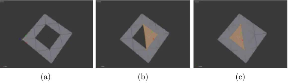
Figure 2.11: These subfigures illustrate different non-manifold meshes. Sub-figure (a) illustrates a non-manifold mesh. This mesh is non-manifold due to the inability to distinguish the inside and outside region of the mesh (i.e it is not a closed surface). Subfigure (b) shows the inside of a cube mesh with additional internal face. This internal face has both of its sides facing the in-terior of the outer model and is therefore a non-manifold mesh. Subfigure (c) illustrates two pyramids connected by a single vertex. This is a non-manifold mesh because the connecting point of the two pyramids can be infinitely small point.
2.5
Kinect Sensor
The Kinect is a motion sensing device created by Microsoft for their home gaming console, the Xbox. This device has an RGB camera and an infra-red camera. Figure 2.12 shows the two iterations of the Kinect so far: the first version for the Xbox 360 and the second for the Xbox One. The infra-red camera allows the Kinect to generate an image that stores the depth infor-mation of the environment. This allows the Kinect to generate two images of the environment, a regular RGB image and a depth image, as shown in Figure 2.13. The outputs from the Kinect are called RGB-D images. The depth image allows us to compute a 3D point for each of the pixels, assuming valid depth data. Some regions of the depth image may be too close or too far for the sensor to correctly detect depth. If this is the case, those regions will be report as zero depth in the image. Assuming the calibration matrix K
CHAPTER 2. BACKGROUND 22
(a) (b)
Figure 2.12: Subfigure (a) illustrates the Kinect for Xbox 360. Subfigure (b) illustrates the Kinect for Xbox One.
(a) RGB image (b) Brightened depth image
Figure 2.13: These figures are the example of the output from the Kinect sensor. Subfigure (a) is a RGB image from the Kinect. Subfigure (b) is (a brightened version of) the depth image.
Section 2.1.2.
2.5.1
Generating the World
The Kinect can be used to rebuild the world over time as a sequence of point clouds from the perspective of the Kinect. This is done by capturing a sequence of RGB-D images I1. . . Ii. . . In, then generating a point cloud P1. . . Pi. . . Pn corresponding to each image. Each of these generated point clouds contains a collection of points from the perspective of the Kinect at a given time step. If the position and orientation of the camera is known for when each of the RGB-D images were taken, then the point clouds can in principle be trans-lated, rotated and combined, assuming the scene is stationary (Hartley and Zisserman, 2004). This will in theory provide a single point cloud that repre-sents all the captured information about the 3D environment. Essentially this
CHAPTER 2. BACKGROUND 23
is the approach employed in the first part of the proposed system discussed in this thesis.
2.6
Summary
This chapter outlined key mathematical methods and concepts used in the thesis. This included the concept of the pinhole camera, which allows for transformations between world coordinates and image coordinates, as well as transformation matrices and quaternions for representing translation and ro-tations. This was followed by approaches to solving linear and non-linear least squares problems. The basic concepts of 3D modelling were introduced and an overview of the Kinect sensor was provided. The next chapter reviews existing techniques that are used for 3D reconstruction and mesh generation.
Chapter 3
Related Work
This chapter discusses work that has been done in previous systems for re-constructing 3D environments, including the problems encountered and solu-tions explored by other researchers. The problem of environment reconstruc-tion is generally stated as the simultaneous localisareconstruc-tion and mapping problem (SLAM). Typically, the trajectory of the camera needs to be recovered and the environment rebuilt at the same time. However, if this is not the case and the poses are known, this is referred to as mapping with known poses. This chapter reviews a number of solutions to the SLAM problem. Following this, alternative approaches to 3D reconstruction are discussed. After tackling the problem of 3D reconstruction, a series of techniques for generating meshes from point clouds are discussed.
3.1
Motion Estimation
Motion estimation is the process of computing the transformation between sequential 2D images. Motion estimation problems are generally addressed using hardware solutions, including mounting sensors such as optical encoders and magnetic sensors to provide odometry. These sensors can be mounted on a robot or vehicle to provide an estimation of motion during data capture. This is used in combination with inertial motion units to detect changes in orientation and estimate the vehicle’s rotation.
The proposed system considers using a hand-held camera which does not capture odometry information thus we only discuss approaches of this kind. The techniques referred to below are often called registration or scan-matching. They operate by ‘registering’ the initial or source image to a ‘reference’ or destination image, which computes the motion from the initial image to the reference. Each of these images can be converted to a set of points in 3D space.
CHAPTER 3. RELATED WORK 25
Iterative Closest Point
The iterative closest point (ICP) algorithm uses multiple techniques to com-pute the motion between two sets of points. The algorithm has many variants since parts of the algorithm can be replaced by alternative techniques. The ICP algorithm has three iterated stages: the first is point association, the second is point rejection, and the last is a minimisation step. ICP works by iteratively attempting to make new associations between different point pairs and minimise an error function during each iteration. There are multiple ways in which the point associations, the point rejections and the minimisation of the error function can be performed. Rusinkiewicz and Levoy (2001) have compared various combinations of these approaches to find the most efficient variants of ICP.
The first variant of ICP, detailed in Besl and McKay (1992), creates its association between the two sets of points by computing the Euclidean distance between a point from the first set to each point in the second. The point in that second set that has the smallest distance is associated with the point in the first set. At this stage associations with a large value can be discarded if necessary as the point rejection step, depending on the overlap area that the two point sets have. After this, the ICP algorithm attempts to minimise an error function that computes the estimated transformation matrix from the first point set to the second. The transformation is estimated in two parts, the first attempting to compute the quaternion that represents the rotational component of the transformation by using the approach in Horn (1987). The algorithm then estimates the translation component as the change in the centres of mass between the point clouds to construct the estimated transformation matrix. The point cloud is transformed by the estimated transformation matrix and the process is repeated by performing all three stages again due to the point association technique used. The association technique has no way to ensure that the matches are correct and thus its results are iteratively refined. Then a point-to-point error metric is used to determine the quality of the estimated transformation in which the sum of the squared distance between points in each correspondence pair is calculated. This process stops once the error has reduced to an acceptable tolerance or a certain number of iterations have passed.
The next approach by Low (2004) replaces the point association and min-imises a different error function compared to Besl and McKay (1992). To create the association, a projective data association approach is used. Two depth images are used to store the point cloud data and the association is made between their pixels. This occurs by projecting a pixel from the source depth image onto the target image; the position where the projection lands is the associated pixel. Since this method uses a projective data association tech-nique, it requires that the changes between the two images be relatively small
CHAPTER 3. RELATED WORK 26
because linearisation is performed during motion estimation. This technique uses the associated pixels from the depth images to compute the 3D position of each pixel. Once the associations of the 2D pixels are made and are con-verted to 3D, the point-to-plane error metric is used (Chen and Medioni, 1992). The point-to-plane error metric aims to minimise the sum of the squared dis-tance between the source point and the tangent plane at its correspondence destination point. The point-to-plane error metric allows point rejection by testing two metrics; the similarity between the tangents to the source and des-tination point and the Euclidean distance between these points. If tangents deviate beyond a threshold or the euclidean distance exceeds a set threshold, the point pairs are rejected. This technique is used in the proposed system, and is further discussed in Section 5.4.
The scan-matching techniques often only use a subset of points that have strong associations between them to improve robustness and reduce computa-tional complexity. However, other techniques such as Steinbr¨ucker, Sturm and Cremers (2011) make use of all the pixels present in an image. Steinbr¨ucker, Sturm and Cremers (2011) present an energy-based approach for RGB-D im-ages. An energy function is presented that aims to obtain the best rigid body transformation from one RGB-D image to the other. This technique aims at minimizing the back-projection error to find a rigid body transformation from the special Euclidean group SE(3) representing the camera motion such that the second image exactly matches the first. For large motion this tech-nique implements a coarse-to-fine approach iteratively improving on the rigid body transformation. The presented approach was compared to a state-of-the-art implementation of ICP known as Generalized-ICP (GICP). GICP proved more robust with larger camera motion than the technique presented; how-ever, Steinbr¨ucker, Sturm and Cremers (2011) provided more accurate results in regions of smaller motion while being faster than the GICP method.
Huang and Bachrach (2017) use a feature-based approach to achieve real-time motion estimation using the Kinect sensor. This technique is designed to operate on a low cost device mounted on a quadrocopter to estimate its local position and stabilize the quadrocopter for autonomous flight. This approach combines multiple techniques to provide high performance with six stages to the motion estimation: The first stage is image preprocessing, where the in-coming depth image is processed through a Gaussian filter, the RGB image is converted to greyscale and a Gaussian pyramid is constructed. This allows the detection of features on a larger scale. The second stage is feature extraction; the FAST (Rosten and Drummond, 2006) feature extractor is used on each level of the pyramid to extract the features, and the depth image is used to extract the associated depth. The third stage is generating an initial rotation estimate; this is performed using a homography-based 3D tracking algorithm (Mei, Benhimane, Malis and Rives, 2008). This technique computes a warping function that is used to warp the source image to the target image. This
al-CHAPTER 3. RELATED WORK 27
lows the system to constrain the search window for the feature-matching. This stage could also use the addition of an IMU to compute the initial rotation. The next stage is feature matching, which computes the sum of the differences between the pixels of the feature from the source image and the destination image (Howard, 2008) as the metric for feature similarity. The fifth stage is in-lier detection; this ensures that the Euclidean distance between two features at one time should match their distance at another time. Finally, stage six does the final motion estimation using Horn’s absolute orientation method (Horn, 1987) to compute rotation and a non-linear least squares solver to minimise the reprojection errors of features in the environment.
Estimating the motion of the camera using ICP is generally performed using an inter-frame approach. This is done by using one image as the reference frame and computing the motion from the reference frame to the next frame called the target. Computing the camera’s motion in this way causes the location estimate to drift as the motion errors accumulate for every image processed. To prevent this from happening, the system needs to correct this drift using SLAM techniques and loop closure techniques.
3.2
SLAM Solutions
Rebuilding scenes in 3D requires knowing the position of the camera and the distance from the sensor to objects in the scene. The simultaneous localization and mapping problem (SLAM) was originally formalized in 1986 by Smith and Cheeseman (1986) in which a generalised method for estimating the spatial location of objects was presented, followed by improvements in Smith, Self and Cheeseman (1987). Informally, the SLAM problem involves determining where a given robot or vehicle is within an environment while simultaneously mapping the environment. This section outlines a number of approaches to tackling the SLAM problem.
Informally SLAM works by tracking key features, known as landmarks, detected in images or other sensory data to determine the camera or sensor’s position and orientation. In an extreme case, every pixel of an image might be considered a landmark.
A probabilistic formulation of SLAM was pioneered in the work of Smith and Cheeseman (1986) on probabilistic spatial representation. This laid the groundwork for a 6 degrees of freedom model for estimating relationships be-tween camera position and environmental objects in three dimensions, as well as the associated uncertainty. Durrant-Whyte (1988) produced work on trans-forming the uncertain points, curves, and surfaces from one coordinate frame to another.
Major breakthroughs occurred in the late 1990’s and early 2000’s due to the decreasing price of sensory devices and faster processors. This gave standard