Ecient Reliability Modelling & Analysis of
Complex Systems with Application to
Nuclear Power Plant Safety
Thesis submitted in fullment of the requirements of the University of Liverpool and the National Tsing Hua University, for the degrees
of Doctor of Philosophy in Engineering and Nuclear Engineering, respectively
by
Hindolo George-Williams (B.Eng(Hons), Electrical/Electronic Engineering and M.Sc(Eng), Energy Generation)
Dedication
Acknowledgement
I thank God the Almighty Father, for His unfailing love and divine favour during my research. I thank, also, the Liverpool School of Engineering and the College of Nuclear Science - National Tsing Hua University in Taiwan, for funding the research reported in this thesis. The series of trainings I received from the Engineering and Physical Sciences Research Council (EPSRC) Centre for Doctoral Training (CDT) on the Quan-tication and Management of Risk & Uncertainty in Complex Systems & Environments are invaluable. For this, I express my sincere gratitude to the management of the CDT. I would be remiss to not acknowledge the unwavering support, guidance, and atten-tion I received from my supervisors, Dr. Edoardo Patelli and Prof. Min Lee. They did an excellent job shaping the direction of my research and most importantly, putting up with my many questions and sometimes tenacious tendencies, when it came to my work. My relationship with Dr. Patelli, especially, has evolved over the years to transcend the usual student-supervisor relationship. This, on its own, went a long way to creating a relaxed and friendly research environment, one in which I expressed my opinions freely. My research would not have been as interesting and smooth, without the love and support I received from my friends, parents, and siblings. They were always there for me, and for this, I thank them. To my wife Henrietta, words can not quite express how grateful I am for your understanding, love, and care. Even when it was this very research that kept us apart for years, you never complained, instead, you encouraged me to dedicate as much time to it as was required. You couldn't have been more supportive! Finally, I thank Hector Diego Estrada-Lugo, Owen Kai-Combey, Ikenna Okaro, and Uchenna Oparaji, for proofreading this thesis.
Abstract
Nuclear power may be our best chance at a permanent solution to the world's energy challenges, owing to its sustainability and environmental friendliness. However, it also poses a great risk to life, property, and the economy, given the possibility of severe accidents during its generation. These accidents are a result of the susceptibility of the generating plants to component failure, human error, extreme environmental events, targeted attacks, and natural disasters. Given the complexity and high interconnectivity of the systems in question, a small glitch, otherwise known as an initiating event, could cascade to catastrophic consequences. It is, therefore, vital that the vulnerability of a plant to these glitches and their ensuing consequences be ascertained, to ensure that the appropriate mitigating actions are taken.
The reliability of a system is the likelihood that it survives a dened period and its availability is the likelihood of it being capable of performing its required functions on demand. These quantities are important to a nuclear power plant's safety because, a nuclear power plant by default is equipped with safety systems to inhibit the propaga-tion of an initiating event. An accident ensues if the safety systems required to mitigate some initiating event are unavailable or incapacitated by the initiating event. It is, therefore, easy to see that the reliability, as well as the availability of these systems, shape the safety of the plant. These crucial quantities, currently, are estimated using legacy techniques like static fault and event tree analyses or their derivatives. Despite their popularity and widely acclaimed success, these legacy techniques lack the exi-bility to implement fully the operational dynamics of the majority of systems. Most importantly, their ease of application deteriorates with increasing system size and com-plexity, such that the analyst is often forced to make unrealistic assumptions. These unrealistic assumptions sometimes compromise the accuracy of the results obtained and subsequently, the quality of the risk management decisions reached. Their inadequacy is often amplied if the system is composed of multi-state components or characterised by epistemic uncertainties, induced by vague or imprecise data. The ideal approach, there-fore, should be suciently robust to not necessitate unrealistic assumptions but exible enough to accommodate realistic system attributes, while guaranteeing accuracy.
This dissertation provides a detailed account of a series of computationally ecient system reliability analysis techniques proposed to address the limitations of the existing
probabilistic risk assessment approaches. The proposed techniques are based mainly, on an advanced hybrid event-driven Monte Carlo simulation technique that invokes load-ow principles to resolve, intuitively, the diculties associated with the topological complexity of systems and the multi-state attributes of their components. In addition to their intuitiveness and relative completeness, a key advantage of the proposed techniques is their general applicability. They have been applied, for instance, to a variety of problems, ranging from the production availability of an oshore oil installation and the maintenance strategy optimization of the IEEE-24 bus test system to the probabilistic risk assessment of station blackout accidents at the Maanshan nuclear power plant in Taiwan. The proposed techniques, therefore, should inuence robust decisions in the risk management of not only nuclear power plants but other critical systems as well. They have been incorporated into the open-source uncertainty quantication tool, OpenCossan, to render them readily available to industry and other researchers.
Declaration
I declare that this thesis was composed by myself and that the results contained herein have not been submitted for any other degree or professional qualication. I conrm that the work submitted is mine, except where it forms part of a jointly authored pub-lication. In which case, my contribution and the names of the other authors have been explicitly indicated below. I conrm also that appropriate credit is given where reference is made to others' work and that the thesis contains 216 pages, 91 gures, and 30 tables. The work in Chapter 7 is under consideration for publication in the Proceedings of the Institution of Mechanical Engineers, Part O: Journal of Risk and Reliability as "Extending the survival signature paradigm to complex systems with non-repairable dependent failures" with co-authors, G. Feng, F.P.A Coolen, M. Beer, and E. Patelli (supervisor). The framework was conceived by all the authors and I, in addition, carried out its algorithmic implementation and prepared the rst draft of the manuscript.
List of Publications
Peer-reviewed Journal Publications
1. H. George-Williams and E. Patelli. A hybrid load-ow and event driven simulation approach to multi-state system reliability evaluation. Reliability Engineering & System Safety, 152:351-367, 2016. Available at http://dx.doi.org/10.1016/j. ress.2016.04.002
2. H. George-Williams and E. Patelli. Ecient Availability assessment of recong-urable multi-state systems with interdependencies. Reliability Engineering & Sys-tem Safety, 431-444, 2017. Available at http://dx.doi.org/10.1016/j.ress. 2017.05.010
3. H. George-Williams and E. Patelli. Maintenance strategy optimization for com-plex power systems susceptible to maintenance delays and operational dynam-ics. IEEE Transactions on Reliability, 66(4):1309-1330, 2017. Available at http://dx.doi.org/10.1109/TR.2017.2738447
4. H. George-Williams, M. Lee, and E. Patelli. Probabilistic risk assessment of station blackouts in nuclear power Plants. IEEE Transactions on Reliabil-ity, 67(2):494-512, 2018. Available at http://dx.doi.org/10.1109/TR.2018. 2824620
5. H. George-Williams, G. Feng, F.P.A Coolen, M. Beer, and E. Patelli. Extending the survival signature paradigm to complex systems with non-repairable depen-dent failures. Proceedings of the Institution of Mechanical Engineers, Part O: Journal of Risk and Reliability (Accepted).
Peer-reviewed Conference Publications
1. H. George-Williams and E. Patelli. Monte Carlo-based reliability/availability analysis algorithm for ecient maintenance planning. In Proceedings of the Struc-tural Mechanics in Reactor Technology Conference, Vol. 23, Manchester, 2015.
2. H. George-Williams and E. Patelli. Ecient availability assessment of recong-urable complex multi-state systems with interdependencies. In Proceedings of the European Safety and Reliability Conference, Vol. 26, Glasgow, 2016.
3. H. George-Williams, E. Patelli, and M. Lee. Reliability & performance analysis of multi-state systems based on analytical load-ow considerations. In Proceedings of the European Safety and Reliability Conference, Vol. 26, Glasgow, 2016. 4. H. George-Williams, E. Patelli, and M. Lee. A framework for power recovery
probability quantication in nuclear power plant station blackout sequences. In Proceedings of the Probabilistic Safety Assessment and Management Conference, Vol. 13, Seoul, 2016.
5. E. Patelli, H. George-Williams, J. Sadeghi, R. Rocchetta, M. Broggi, M. de An-gelis. OpenCossan 2.0: an ecient computational toolbox for risk, reliability, and resilience analysis. In Proceedings of the 7th International Symposium on Uncertainty Modelling and Analysis, Florianapolis, 2018.
Contents
Dedication i Acknowledgement iii Abstract v Declaration ix List of Publications xi Nomenclature xixList of Figures xxvii
List of Tables xxx
1 Introduction 1
1.1 Background . . . 1
1.2 Complex System Reliability . . . 2
1.3 Motivation . . . 2
1.3.1 The Role of System Reliability Analysis in Nuclear Safety . . . . 3
1.3.1.1 The Three Mile Island Accident . . . 4
1.3.1.2 The Chernobyl Nuclear Disaster . . . 5
1.3.1.3 The Fukushima Daiichi Disaster . . . 5
1.3.1.4 Concluding Remarks . . . 6
1.4 Aims and Objectives . . . 7
1.5 Thesis Structure . . . 7
2 The State of the art in System Reliability & Risk Modelling 9 2.1 Existing Reliability Modelling Techniques . . . 9
2.2 Dependencies in Engineering Systems . . . 12
2.2.1 Forms of Interdependencies . . . 13
2.2.1.2 Cascading Failures . . . 15
2.3 Maintenance Modelling of Complex Systems . . . 16
2.3.1 Maintenance Strategy Optimization . . . 16
2.4 Nuclear Power Plant Safety . . . 18
2.4.1 Station Blackout Risk Quantication . . . 19
2.5 The Concept of Survival Signature . . . 20
2.5.1 Theoretical Basics . . . 21
2.5.2 Applications and Limitations . . . 22
2.6 Chapter Summary . . . 23
3 Multi-state System Reliability Modelling & Evaluation 25 3.1 Introduction . . . 25
3.2 Overview of Proposed Approach . . . 26
3.2.1 Advantages Over Existing Techniques . . . 27
3.3 Component Modelling . . . 28
3.3.1 Application to Repairable Multi-state Components and Systems . 30 3.3.2 Determining Component State Transition Parameters . . . 32
3.4 System Modelling . . . 33
3.4.1 The System as a Directed Graph . . . 34
3.4.2 System Representation and Flow Analysis . . . 36
3.4.2.1 Derivation of System Flow Equations . . . 37
3.4.2.2 Output Calculation and Node Reconguration . . . 41
3.4.3 Simulation Procedure . . . 42
3.4.4 Limitations of the Proposed Approach . . . 44
3.5 Case Studies . . . 44
3.5.1 Case Study 1: A Simple Pipe Network . . . 44
3.5.1.1 Analyses . . . 45
3.5.1.2 Results and Comments . . . 48
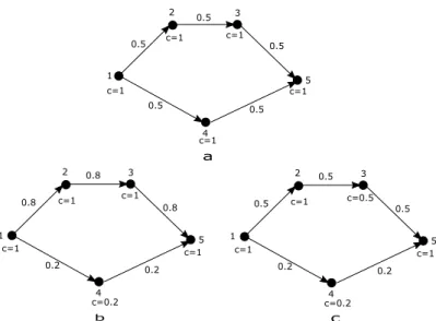
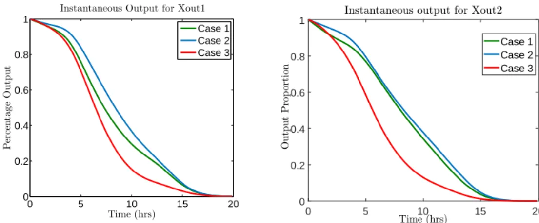
3.5.2 Case Study 2: A Multi-State Bridge Network . . . 48
3.5.2.1 Analyses . . . 49
3.5.2.2 Results and Comments . . . 51
3.5.3 Computational Cost of Approach . . . 53
3.6 Chapter Summary . . . 54
4 Availability Assessment of Interdependent Multi-state Systems 55 4.1 Introduction . . . 55
4.2 Overview of Proposed Approach . . . 56
4.3 Implementation . . . 57
4.3.1 Decoupling the System . . . 58
4.3.3 Node Reconguration . . . 62
4.3.4 Determining system performance at time t . . . 62
4.4 The System Simulation Procedure . . . 63
4.4.1 Forcing Maintenance . . . 64
4.4.2 Maintenance Priority & Real-time Component Ranking . . . 65
4.4.3 The Simulation Algorithm . . . 66
4.5 Obtaining the Availability and Performance Indices . . . 67
4.5.1 System Reliability and Recovery Probability . . . 68
4.5.2 Instantaneous Availability and Expected System Output . . . 69
4.5.3 Maintenance Response Inadequacy . . . 71
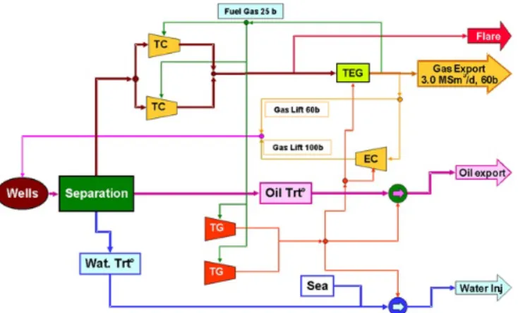
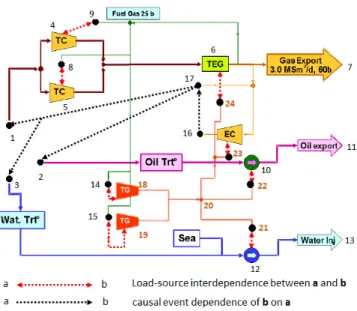
4.6 Case Study: An Oshore Oil Installation . . . 72
4.6.1 Problem Formulation . . . 72
4.6.1.1 Interdependencies & Reconguration . . . 73
4.6.1.2 Maintenance Policy . . . 73
4.6.1.3 Monte Carlo Simulation . . . 74
4.6.2 Solution Procedure . . . 74
4.6.2.1 Modelling the Plant . . . 75
4.6.2.2 Production Level Determination . . . 77
4.6.3 Simulation Results . . . 77
4.6.3.1 Expected Production . . . 81
4.6.3.2 Reliability and Recovery . . . 81
4.6.3.3 Eects of Real-time component ranking . . . 82
4.6.3.4 Eects of limited maintenance teams . . . 83
4.6.4 Comments and Discussions . . . 83
4.7 Chapter Summary . . . 84
5 Probabilistic Risk Assessment of Station Blackout Accidents 87 5.1 Introduction . . . 87
5.2 The Proposed Approach and Scope . . . 88
5.2.1 Merits & Novelty of Proposed Approach . . . 88
5.2.2 Solution Sequence . . . 89
5.3 Station Blackout Modelling . . . 89
5.3.1 The System Topology . . . 89
5.3.2 The System Components . . . 91
5.3.2.1 Modelling the Grid and Switchyard . . . 91
5.3.2.2 Modelling the Standby Power Systems . . . 92
5.3.2.3 Accounting for Human Error . . . 94
5.3.3 Modelling Component Interdependencies . . . 96
5.3.3.1 The CCF Model . . . 96
5.4 System Simulation & Analysis . . . 99
5.4.1 SBO Indices: Computation & Relevance . . . 100
5.4.2 Incorporation into the Existing Framework . . . 101
5.5 Case Study:The Maanshan Nuclear Power Plant . . . 102
5.5.1 Developing the System and Component Models . . . 103
5.5.2 Component Reliability Data . . . 105
5.5.3 Representing Component Interdependencies . . . 107
5.5.4 Results and Discussions . . . 110
5.6 Chapter Summary . . . 113
6 Maintenance Strategy Optimization for Complex Power Systems 115 6.1 Introduction . . . 115
6.1.1 Advantages of the Proposed Approach . . . 116
6.2 Problem Formulation . . . 117
6.2.1 Denition of key terms . . . 119
6.2.2 The Cost Model . . . 120
6.2.3 Proposed Maintenance Regimes . . . 122
6.2.4 Solution Sequence . . . 123
6.3 System Reliability and Performance Analysis . . . 124
6.3.1 Component and System Representation . . . 125
6.3.2 Maintenance Modelling of Components . . . 125
6.3.3 Determining Component Transition Parameters . . . 130
6.3.3.1 Accounting for Non-Markovian Transitions . . . 130
6.3.4 Maintenance Strategy Implementation . . . 132
6.3.5 The Simulation Procedure . . . 134
6.4 Case-Studies . . . 137
6.4.1 Case-Study 1: A 50MW Hydroelectric Power Plant . . . 137
6.4.1.1 Modelling the Plant and its Components . . . 138
6.4.1.2 The Eects of Maintenance on System Performance and Reliability . . . 139
6.4.1.3 Optimal Maintenance Strategy Identication . . . 141
6.4.1.4 Sensitivity to Cost Levels . . . 142
6.4.1.5 Computational costs . . . 142
6.4.1.6 Discussions . . . 142
6.4.2 Case-Study 2: The IEEE-24 Bus Reliability Test System . . . 144
6.4.2.1 Maintenance Information . . . 146
6.4.2.2 Maintenance Grouping and Costs . . . 147
6.4.2.3 Objective . . . 147
6.4.2.4 System modelling . . . 147
6.4.2.6 Results and Discussions . . . 150
6.5 Chapter Summary . . . 152
7 An Extended Survival Signature Approach for Dependent Failures 155 7.1 Introduction . . . 155
7.2 Overview of Proposed Approach . . . 156
7.3 Modelling & Simulating the System . . . 156
7.3.1 Components with Multiple Failure Modes . . . 156
7.3.2 Cascading Failure Modelling and Propagation . . . 158
7.3.3 CCF Modelling and Propagation . . . 159
7.3.4 The Simulation Algorithm . . . 162
7.3.5 Sensitivity Analysis . . . 164
7.4 Case Studies . . . 164
7.4.1 Case Study 1: A Complex Bridge Network . . . 165
7.4.1.1 Analyses and Results . . . 165
7.4.1.2 Discussions . . . 167
7.4.2 Case Study 2: A Hydroelectric Power Plant . . . 168
7.4.2.1 Analyses and Results . . . 170
7.4.2.2 Discussions . . . 171
7.5 Chapter Summary . . . 172
8 Conclusions 173 8.1 Concluding Remarks . . . 173
Nomenclature
ABBREVIATIONS
AC Alternating Current.
BDD Binary Decision Diagrams.
BPM Basic Parameter Model.
CCF Common-Cause Failures.
CCG Common-Cause Group.
CFT Condition-based Fault Trees.
CM Corrective Maintenance.
DC Direct Current.
DFG Dynamic Flow Graphs.
DFT Dynamic Fault Trees.
DRBD Dynamic Reliability Block Diagrams.
EDG Emergency Diesel Generator.
EENS Expected Energy Not Supplied.
FT Fault Trees.
LOOP Loss Of Osite Power.
MC Markov Chain.
MGL Multiple Greek Letter.
MTTF Mean Time To Failure
NP Non-Polynomial time.
PM Preventive Maintenance.
PN Petri Nets.
RBD Reliability Block Diagrams.
RG Reliability Graphs.
SBO Station Blackout.
SDP Sum of Disjoint Products.
UGF Universal Generating Function.
NOTATIONS
AB Elements inA but not in B.
Bpónq Next nrows of matrixB.
pA, mÑnq Elements mto nof vector A.
pB, iq ith element of vectorB.
pEEN Sqef f Total system EENS.
ra, bs Maintenance strategy based on regimes aandb. Exppaq Exponential distribution with rate1{a.
fptqsk Generate krandom samples from fptq.
Gpa, bq Gamma distribution with shape and scale parameters aand b. Gupa, bq Gumbel distribution with mean,aand standard deviation,b. LpC, Rpn, kqq System loss corresponding to maintenance strategyk.
LogNpa, bq Log-normal distribution with mean, aand standard deviation,b. minpB, bq The least element ofB greater thanb.
minpBq The least element of vectorB.
numelpBq Number of elements in set/vector B.
Rpn, kq System reliability and performance indices for maintenance strategyk. sizepB,1q Number of rows of matrix B.
Upa, bq Uniform distribution with bounds onaand b. u p0,1q Uniform random number between 0 and1.
W bpa, bq Weibull distribution with scale and shape parameters aand b.
APM Awaiting preventive maintenance state.
CPHM Cost per Hour of Maintenance.
CS Cold Standby state.
EC Electricity Cost.
F Failed state.
FMC Fixed Cost per Maintenance team.
I Idle state.
PF Partial failure state.
S Shut-down state.
SU Start-Up state.
TM Test/Maintenance state.
W Working state.
SYMBOLS
αij Transmission eciency of link between nodes iandj.
β1tku Common failure mode of CCG k.
β2tku State rendering CCG ksusceptible to CCF.
β Matrix of possible system component combinations.
δ Set of components in shut-down.
η Vector of system node ows.
Γ System incidence matrix.
fi Set of nodes sending ow to nodei.
µ Vector of current capacities of system nodes.
ν Shared/dedicated maintenance indicator vector.
Φ System equality constraint matrix.
Π Matrix dening the size of each maintenance group.
Ψ Vector of system performance history.
ρtku Set of typek components.
τ Vector of next transition times of nodes.
τpm Vector of next preventive maintenance due times of components.
τspare Vector of component spares availability times.
Θ System inequality constraint matrix.
θtku CCF probabilities for CCGk.
θj Total set of components in maintenance groupj
θtjcmuYθtjpmu . θtjcmu Set of components assigned to group j for CM.
θtjpmu Set of components assigned to group j for PM.
ς Component sink index vector.
ϑ1 Set of components repaired only while in shut-down.
ϑ2 Set of components which PM is initiated only while in shut-down.
A System adjacency matrix.
C Component capacity vector.
D1i Joint dependency matrix of node i.
Di Dependency matrix of node i.
e System edge matrix
ht Global set of components in maintenance queue.
h1f Final content of h1 after normalization.
h1 Set of components in CM queue.
h2f Final content of h2 after normalization.
h2 Set of components in PM queue.
I Indicator register for subsystems aected by the last node transition.
lb Vector of minimum ow across links.
L System capacity matrix.
n Combination of maintenance teams.
R Set of ranks of subsystems associated with a node.
s Set of source nodes.
Sτ System survival signature.
Si Set of nodes belonging to subsystemi.
T Transition matrix of component.
t Set of sink nodes.
ttimes Set of sampled transition times.
V Set of system nodes.
χ Number of power trains generator can supply simultaneously.
δ System time step.
δt Total number of system time steps.
ηi Flow through node i.
ð Number of intermediate nodes.
Λ Minimum load rating of component.
λ1 Total number of busy corrective maintenance teams.
λ2 Total number of busy preventive maintenance teams.
λt Total number of busy maintenance teams.
λtjcmu Number of busy CM teams in groupj. λtjpmu Number of busy PM teams in group j. λmn Failure rate from statem to n.
C Cascading matrix.
Di Set of dual nodes of nodei.
E Set of component properties.
Ei Properties of componenti.
F Set of failed components/nodes.
H Matrix of CCF probabilities.
H1 Cumulative sum ofHalong rows.
Ii Set of components which failure is induced by component i.
Li Load dependency parameter of nodei.
N Set of all possible maintenance team combinations, tn1,n2, ...,nφu.
O Objective function.
T Vector of system transition times.
µticmu Indicator function for CM suspension of component i. µtipmu Indicator function for PM suspension of component i. µmn Repair rate from state mto n.
ω Total number of system maintenance groups.
Ωij Maximum ow from node ito nodej.
X Set of system state vectors corresponding tox1.
x System state vector.
x1 Modied system state vector.
xk State vector for group of type kcomponents. εx Sink index of component in statex.
εtxiu Sink index of componentiin state x.
ϕpxq System structure function.
ξ Set containing the size of each component group. Aptq Instantaneous system availability.
Citcmu Cost per hour of corrective maintenance of componenti. Citpmu Cost per hour of preventive maintenance of component i.
cmax Maximum capacity of component.
Csticmu Unit cost of CM spares for component i.
Cstipmu Unit cost of PM spares for componenti.
ctxiu Capacity of node ibefore state transition.
ctxiu Current capacity of component i.
eij Link/edge between nodesiand j.
fl LOOP frequency.
fs SBO frequency.
fxyptq Probability density function of transition time from statex to y.
G System graph model.
K Number of component types.
k Number of edges in system graph.
kf Multiplication factor.
ki Proportion of PM duration of component ispent before interruption.
lij Capacity of link/edge between nodes iand j.
M Total number of system nodes.
m Total number of power trains.
M1 Total number of maintainable components.
M2 Number of external nodes.
mj Number of components assigned to maintenance group j.
Mk Number of typek components.
N Number of simulation samples.
n Number of component states.
n1 Total number of corrective maintenance teams.
n2 Total number of preventive maintenance teams.
nt Total number of maintenance teams.
n1j Number of corrective maintenance teams in groupj.
n2j Number of preventive maintenance teams in groupj.
Nitcmu Number of successful corrective maintenance actions on component i. Nitpmu Number of successful preventive maintenance actions on componenti. ntj Total number of maintenance teams in groupj.
Ppx1q Occurrence probability of x1.
pt1sbou Conditional SBO probability given LOOP.
ptnsbou Conditional nth SBO probability given the pn1qth SBO.
ptisu Probability of spares being used in the repair of component i. pz Average probability of state z.
pzptq Instantaneous probability of state z.
r1ptq System non-recovery probability.
r21 ptq Non-recovery probability from second SBO. rptq System recovery probability.
Rptq System reliability.
sj SBO indicator forjth simulation sample.
sticmu Number of spares used for corrective maintenance of component i. stipmu Number of spares used for preventive maintenance of component i. t1 Maximum remaining lifetime of a component in APM state.
Tm Mission time.
tticmu Time spent by component iin corrective maintenance. ttipmu Time spent by component iin preventive maintenance.
tnext Next transition time.
tpm Component expected preventive maintenance duration.
tsample Minimum sampled transition time.
tspent Time spent in shut-down.
u Proportion of power train demand demand generator satises. Utm Unavailability due to test or maintenance.
x Current state of component.
x1k Number of available type kcomponents. Xptq Expected instantaneous system output.
x0 Initial state of component.
xi State ofith component.
xs State of system.
Xij Flow across link/edgeeij.
y1 Next failure state of a component in APM state.
ym Next maintenance state.
List of Figures
1.1 Thesis structure and relationships between chapters. . . 7 2.1 Forms of interdependencies in engineering systems. . . 13 3.1 State-space diagram of a particular multi-state component. . . 28 3.2 State-space diagram of 40MVA generator. . . 30 3.3 Alternative state representation of generator. . . 31 3.4 Flow visualisation in a particular 5 node system. . . 37 3.5 A 3-component pipe network. . . 45 3.6 Network model of pipe network. . . 45 3.7 State-space diagram of components. . . 47 3.8 Reliability function. . . 47 3.9 System instantaneous output. . . 47 3.10 Block diagram of test bridge network. . . 48 3.11 State-space diagram of system nodes . . . 49 3.12 Graph for case 1. . . 50 3.13 Graph model for cases 2 & 3. . . 50 3.14 Failure time dist. at Xout1. . . 51 3.15 System reliability at Xout1. . . 51 3.16 System reliability at Xout2. . . 51 3.17 System reliability at Xout3. . . 51 3.18 Instantaneous output at Xout1. . . 52 3.19 Instantaneous output at Xout2. . . 52 3.20 Instantaneous output at Xout3. . . 52 3.21 Performance indices at Xout3. . . 52 3.22 Allocation for case study 1. . . 53 3.23 Allocation for case study 2. . . 53 4.1 An example of a typical interdependent system. . . 57 4.2 Interdependent system showing load-source pairs. . . 59 4.3 Dependency tree for a 4-subsystem system. . . 60
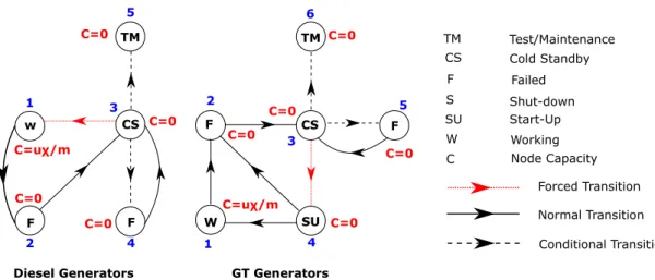
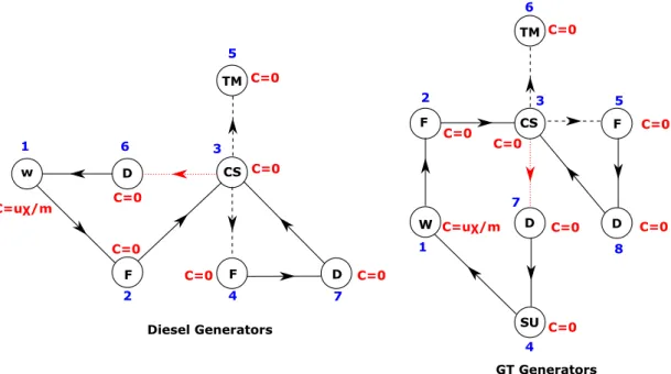
4.5 Dependency tree for sample interdependent system. . . 61 4.6 System performance history for one Monte Carlo realisation. . . 67 4.7 System performance history showing failure and recovery times. . . 67 4.8 Bounds on maintenance response inadequacy of a sample system. . . 71 4.9 Schematic of an oshore installation. . . 72 4.10 State-space diagrams of components. . . 72 4.11 State-space for EC and TEG. . . 74 4.12 State-space for TC and TG. . . 74 4.13 System model showing dependencies. . . 75 4.14 Plant network model. . . 76 4.15 Expected instantaneous plant performance under CM only. . . 79 4.16 Expected instantaneous plant performance under CM and PM. . . 80 4.17 Plant availability relative to state 1. . . 80 4.18 Plant reliability and recovery probability relative to state 1. . . 81 4.19 Maintenance response inadequacies for one CM team. . . 82 5.1 Multi-state model for Grid and Switchyard nodes. . . 92 5.2 Models for emergency diesel and gas turbine generators without human
error. . . 93 5.3 Multi-state model for switchyard with human error consideration. . . 94 5.4 Models for emergency diesel and gas turbine generators with human error. 95 5.5 An excerpt from the SBO event tree showing headings. . . 101 5.6 Layout of the Maanshan nuclear power plant AC distribution system. . . 102 5.7 Simplied schematic of plant's AC distribution system. . . 103 5.8 Multi-state model for the main diesel generators (DG-A & DG-B). . . . 104 5.9 Multi-state model for the shared diesel generator (DG-5). . . 104 5.10 Multi-state model for the gas turbine generators (GT1 & GT2). . . 105 5.11 Full system graph model showing maximum ow along links. . . 105 5.12 Eective repair CDF for multiple grid sources. . . 105 5.13 Eective repair CDF for multiple switchyard sources. . . 105 5.14 Probability of SBO duration exceedance. . . 111 5.15 Composite frequency of rst SBO exceedance. . . 111 5.16 Comparison of composite frequencies of exceedance. . . 112 5.17 Comparing SBO frequencies. . . 112 5.18 Comparing 2nd SBO probs. . . 112
6.1 State-space of a binary-state component under various maintenance sce-narios. . . 125 6.2 Repairable binary-state component under maintenance delays. . . 126
6.3 Binary-state component under `maintenance only when component is un-available'. . . 128 6.4 Multi-state component under maintenance delays and operational
uncer-tainties. . . 128 6.5 Schematic of a 2-unit hydroelectric power plant. . . 137 6.6 Plant's network model. . . 138 6.7 State-space diagrams of components. . . 138 6.8 Plant output performance. . . 139 6.9 Plant reliability. . . 139 6.10 Optimal maintenance team size sensitivity to costs. . . 141 6.11 Optimal system loss sensitivity to cost-level variation. . . 141 6.12 Sensitivity of optimal solution to concurrent variation in FMC and CPHM.143 6.13 Single-line diagram of the IEEE-24 bus Reliability Test System. . . 145 6.14 System graph model. . . 148 6.15 Simplied multi-state model for binary-state components. . . 149 6.16 Simplied multi-state model for multi-state generation units. . . 149 6.17 Optimal maintenance team sensitivity to cost levels. . . 150 6.18 System loss sensitivity to cost levels. . . 152 7.1 An arbitrary multi-component complex network. . . 164 7.2 System reliability with dependencies ignored. . . 166 7.3 System reliability with dependencies considered. . . 166 7.4 System reliability sensitivity to CCGs. . . 166 7.5 Sensitivity of critical CCG to component MTTF. . . 166 7.6 Schematic of a 50MW hydroelectric power plant. . . 168 7.7 Condensed block diagram of the plant. . . 168 7.8 Plant block diagram showing interdependencies. . . 169 7.9 Plant reliability with dependencies ignored. . . 170 7.10 Plant reliability with dependencies considered. . . 170 7.11 The eects of dependencies on plant reliability. . . 171
List of Tables
3.1 System node properties. . . 50 3.2 Reliability indices for Xout1. . . 50 3.3 Actual computational cost per case study. . . 53 4.1 Component repair priority. . . 73 4.2 Component preventive maintenance schedule. . . 74 4.3 Production levels of individual commodities. . . 78 4.4 Gas production level probabilities. . . 78 4.5 Oil production level probabilities. . . 78 4.6 Water production level probabilities. . . 78 4.7 Plant production levels identied. . . 78 4.8 Comparison of plant production level probabilities. . . 79 4.9 Expected annual production. . . 81 4.10 Expected annual production compared with Zio's result. . . 81 4.11 Maximum gains from maintenance team scale-up. . . 83 5.1 Human error probabilities for GT1 & GT2. . . 106 5.2 Component Reliability Data. . . 106 5.3 Common-Cause Group Denition. . . 107 5.4 Summary of the static SBO indices obtained. . . 110 6.1 Component state assignment . . . 126 6.2 Description of state transitions . . . 127 6.3 Component and system data for the hydroelectric power plant. . . 137 6.4 Plant expected output and loss. . . 140 6.5 Optimal plant loss as a function of maintenance strategy . . . 141 6.6 Optimal maintenance strategy sensitivity to costs. . . 141 6.7 Maintenance data for generation units. . . 145 6.8 Maintenance costs for generation units. . . 146 6.9 Optimal System Loss as a function of maintenance strategy. . . 150 7.1 Failure time distribution data and CCF parameters of component groups. 165 7.2 Comparison of computation times (in seconds). . . 167
7.3 Failure time distribution data and CCF parameters of plant components. 169 7.4 Comparison of computation times (in seconds). . . 170
Chapter 1
Introduction
1.1 Background
A system is a collection of entities and/or processes working in unison to achieve a common goal. The likelihood of this goal being attained, given a certain operating condition, denes the reliability of that system. One can deduce from this denition that system reliability is relative rather than absolute. It depends on the operating condition of the system, the criteria against which mission success is determined, and the mission duration. For example, a car with a maximum achievable speed of 100km/h would be deemed perfectly reliable for a mission requiring 1000km be covered in 12 hours, barring component failures. The same car, however, under the same conditions, would be absolutely unreliable if the mission were to be completed under 10 hours. Again, if the operating condition were modied to regard component failures, it would be impossible to be certain about mission success, without a detailed and representative reliability analysis of the car. This example highlights the relativity of system reliability. Strictly, a system, as dened earlier, may refer to a biological, nancial, or an engineering system. For the purpose of this thesis, however, it refers to the last of these, and is a collection of mechanical and electronic components. Structural systems like bridges and buildings, which may also be regarded as engineering systems, are outside the scope of this thesis.
An engineering system can be classied along several parameters. For instance, on the basis of its operational period, a system is either continuous or mission-oriented. A mission-oriented system, like a rocket taking essential supplies to the international space station, performs a mission of xed duration [145]. Continuous systems, on the other hand, have an innite mission duration, and their continuity is limited only by their lifespan. Prominent examples include power plants, transportation networks, water distribution systems, and power grids. These systems can also be repairable or non-repairable. Unlike repairable systems, non-repairable systems are built of components that cannot be repaired within the mission. Repairable components are mostly found in
continuous systems and, in fact, are the very reason the systems sustain their continuity. There are many more classications of systems, but these are extensively dealt with in Chapter 2 and the subsequent sections of this chapter.
1.2 Complex System Reliability
A system can be classed as complex from two fronts: complexity in terms of the functional relationships between its components, and complexity due to its struc-ture/topology. A system is deemed structurally complex if it is a series, non-parallel, or non-series-parallel interconnection of components. The components, which are the system's smallest building block, determine its output levels, states, and be-haviour. In realistic systems, these components may exist in one of several possible states/output levels [155], dictated by their failure characteristics, operating conditions, age, or some stochastic event outside the system boundary. The result is a system char-acterised by multiple states, with the number of states determined by the diversity in the states of the components, as well as the structure of the system [38,75].
Unlike binary-state systems which can only be perfectly working or completely failed, multi-state systems can exist in intermediate states, as well. The number of interme-diate states may or may not be nite, depending on the performance measure under consideration and the type of system [75]. For instance, the power generated by a hydroelectric power plant may take any value between zero and its maximum achiev-able value, depending on the height of water in the dam, the performance levels of its components, and the demand on the grid. Other examples of multi-state systems are communication systems; where data processing speed [78, 87] may be the performance measure, cooling systems; where coolant ow rate or cooling capacity [51] may be the performance measure, and production systems; where production rate is the perfor-mance measure. These systems may be standalone or form an indispensable part of some critical system like safety-critical and industrial control systems. It is, therefore, important to be able to assess their susceptibility to failures, quantify, and predict the ensuing consequences, for eective planning of preventive and corrective measures.
Reliability prediction transcends just dening a set of standards for predicting the failure rate of components to system-level and the safety of complex systems [123]. It has phased through tremendous developments, moving from traditional methods treating the failure of a system as a consequence of the failure of its components only, to methods that approach its failure from a wider perspective, including external factors [34].
1.3 Motivation
Failure is an inherent phenomenon in mechanical and electronic components and sys-tems. It is a consequence of their material properties, operating condition, and age.
This highlights the impossibility to innitely operate a system, without scheduled and unscheduled outages. Scheduled outages are due mainly to preventive maintenance and inspections but should be planned in a way that inicts minimal disruptions to the operation of the system. Even though the system operator has no control over when unscheduled outages occur, they can still institute measures to reduce their frequency, mitigate their eects, and ensure the timely recovery of the system when they occur.
An engineering system may be as simple as the smallest circuit in a transistor radio or as critical and complex as an entire nation's transportation, power, communication, and water network. One thing is certain, however, regardless of the size and criticality of a system, its failure is often accompanied by consequences. These consequences range from a mere discomfort (like the one one feels when one's air conditioner is broken) to the more severe phenomena of economic loss and the loss of human lives. In May 2017, for instance, a power failure crippled British Airway's (BA) IT system at the London Heathrow and Gatwick airports in the United Kingdom [21]. The outage, which lasted only a few days, caused hundreds of ight cancellations, leaving about 75,000 passengers stranded, and costing the airline ¿58m [22]. Similarly, in April 2010, the explosion of the Deepwater Horizon drilling rig leased to British Petroleum (BP) in the Gulf of Mexico killed 11 workers, triggering an oil spill believed to be the worst in US history [17]. The disaster did not only bring nancial losses to the company, it created a big dent on its reputation too. In fact, BP were forced to put aside $41bn (more than twice their prot in 2009) to cover clean up costs and legal fees [18]. The reliability analysis, therefore, of engineering systems, is very important, since it is the only way their susceptibility to failures and the ensuing consequences can be quantied.
There are a couple of other reasons why one would want to compute the reliability of a system. At the design stage, for instance, the design engineer would want to ensure a design meets the desired performance and safety requirements or to select the best of multiple designs. After commissioning, a detailed reliability analysis of a system can conrm whether or not it performs as expected and can reveal any vulnerabilities, which information is useful for more robust future designs. There is also maintenance strategy optimization, where a complete reliability analysis of a system is required to compute the benets of possible strategies, and hence, deduce the best maintenance strategy.
1.3.1 The Role of System Reliability Analysis in Nuclear Safety
Nuclear power plants are a typical example of a system that demands the highest reliability of even its smallest component. Some failure events do not only result in their loss of output but sometimes set o a sequence of events with far-reaching consequences as well. The science of examining what can go wrong in a plant and its ensuing risks is known as probabilistic risk assessment (PRA). It entails the identication of the events (known as initiating events) that could trigger unwanted consequences and the
subsequent computation of their frequencies and extent [137]. For nuclear power plants, the primary unwanted consequences are core damage, reactor containment breach, and the release of radioactive materials into the environment. Though these events are extremely unlikely, there have been several nuclear accidents in history, some of which dates to the 1950s [19]. Of these accidents, only the three infamous ones (the Three Mile Island, Chernobyl, and Fukushima Daiichi disasters), however, are explored in this thesis, with focus on their causes, consequences, and similarities.
1.3.1.1 The Three Mile Island Accident
Three Mile Island was a 2-unit pressurised water reactor nuclear power plant in Dauphin county, Pennsylvania. On the 28th day of March 1979, a failure of one of its cooling sys-tems initiated a sequence of events that would later be regarded the most serious nuclear incident in commercial nuclear power generation history in the United States [136]. De-spite its relatively minor health and environmental consequences, however, its aftermath sparked a revolution in the operation, regulation, and emergency response protocols of nuclear power plants in the United States. The accident, rated 5 on the 7-point inter-national nuclear events scale, was initiated by the failure of the main feedwater pumps in the second reactor, which was later traced to imperfect maintenance [62]. Feedwa-ter pumps supply cooling waFeedwa-ter to the steam generator and maintain circulation in the secondary cooling loop of a nuclear reactor. When these pumps failed, the unit's turbine-driven generator and reactor automatically shut down, and the core starved of cooling, began to record a rapid temperature rise. This, in turn, resulted in pressure building up in the reactor, which further actuated the pressure relief valve. However, the valve, which was to reset itself when the pressure fell to an acceptable level, remained stuck open, leading to a loss of coolant accident. Even when the reactor incident alarms went o, the operators did not know a loss of coolant accident was already in progress. In con-sequence, they reduced coolant circulation in the primary cooling loop, which fueled the subsequent partial meltdown of the reactor, due to excessive temperatures [136]. The reactor containment, however, remained intact, and there were no substantial releases of radioactive materials into the surrounding, save for a small amount of radioactive gases in the vicinity of the plant a few days later. These small releases were due to the loss, through the stuck-open valve, of coolant contaminated with radionuclides.
It is clear the accident was initiated by component failure (the failure of the feedwater pumps and the stuck-open valve) but its progression was exacerbated by design decien-cies, human error, and organisational & quality problems [62, 136]. For instance, even when the valve was stuck open, the control instrumentation indicated a closed valve. The operators, prior to the incident, were aware that the valve leaked but postponed its maintenance. Both the valve failure and false indication, therefore, would have been prevented by eective design and maintenance policy reconsiderations.
1.3.1.2 The Chernobyl Nuclear Disaster
The Chernobyl nuclear power plant was a 4-unit graphite-moderated light water reactor, in the Ukrainian city of Chernobyl. Occurring on the 26th of April 1986, the accident, which is arguably the world's worst nuclear disaster, resulted from an experiment-gone-wrong culminating into the explosion of the fourth reactor. The disaster is believed to have released about 2 orders of magnitude more radiation than the atomic bombs dropped on Hiroshima and Nagasaki. More than 350,000 people were resettled and traces of radioactive materials from the accident were found almost everywhere in the northern hemisphere [16]. Two deaths were recorded on the plant premisses, as a direct consequence of the blasts and a further 28 deaths, from exposure to radiation [102].
The accident is attributable to human errors during an experiment to investigate the ability of the fourth reactor to drive its cooling pumps at low power. Executing their plans, the engineers had inserted the control rods into the reactor core, with the view to reducing its power only to about 20% of its nominal value. Too many control rods, however, were introduced, such that the reactor was almost shut down by Xenon poising [129]. In response, the engineers withdrew some rods from the reactor, and in two hours, managed to stabilize the reactor power at about 12% and commenced the test. However, too many rods were withdrawn, and less than 1 minute into the test, the reactor power shot up to about 100 times its nominal value [16]. The reactor's automatic shut-down system which had been disabled to allow the low power operation of the reactor, was reactivated. Its reactivation led to the insertion of more control rods into the core, displacing the mixture of steam and hot coolant that had built up. The result was two catastrophic explosions, blowing away the roof of the reactor building.
Unlike the Three Mile Island accident, component failure had no part in the Cher-nobyl disaster. They, however, share human error and design deciencies, as root causes. In fact, the experiment was scheduled to have been performed by the day shift, who had been trained for the exercise. The night shift, who had very little time to prepare, had to take over after the initial schedule was disrupted by some eventuality. Secondly, the young engineer who was assigned to the control rods had been working indepen-dently for only three months, and may have initiated the accident when he erroneously inserted the control rods too deep. Finally, the consequences of the accident may have been minimized if the reactor were housed in a concrete containment, as present-day reactors are. This was a design inadequacy of the Chernobyl nuclear power plant. 1.3.1.3 The Fukushima Daiichi Disaster
Unlike the Three Mile Island and Chernobyl disasters, the Fukushima accident was triggered by a natural disaster. The accident ensued from a magnitude 9.0 earthquake-triggered 40.5m high Tsunami in east Japan, on the 11th of March 2011 [129]. The tsunami reached about 14m at the 6-unit plant, whose units 4-6 were not in operation
at the time. As a result of the earthquake, the operational reactors automatically shut-down, at which time the backup generators were to take over the powering of the safety systems. These generators, however, were housed in the basement of the turbine building, which was only protected against a 10m ood height. Consequently, the generator room was ooded, initiating a station blackout sequence, culminating into a series of hydrogen explosions that damaged reactors 1-4 [129]. Since the reactors were housed in a concrete containment, the explosions only aected the reactor buildings. The unusual levels of radioactivity recorded in the vicinity of the plant were due to the venting operation employed to relieve the pressure in the respective reactor vessels.
No deaths were linked to the direct exposure to the radioactive nuclides released, but the accident eventually cost the plant operator billions of dollars in compensa-tion claims. Though triggered by natural events, the progression of the accident was largely down to organisational and regulatory deciencies. In fact, the chairman of a Japanese parliamentary panel set up to investigate the accident, Kiyoshi Kurokawa, called it a manmade disaster [20]. The operator had ignored earlier safety concerns about the layout of the emergency cooling system and the vulnerability of the plant to tsunamis. There was no robust probabilistic risk assessment of the plant and the operator's emergency response plan was lacking, the panel found. It is even alleged that relevant sections of the severe accident instruction manual were missing [20].
1.3.1.4 Concluding Remarks
From the preceding reviews, one could argue that nuclear accidents result from at least one of three causes: component failure, natural disasters, and human factors. The human factors may include, but are not limited to, human errors, targeted attacks, negligence, and procedural breaches. Given the unpredictability of these root causes and the potential severity of an accident, probabilistic risk assessment is key to the safe operation of nuclear power plants.
Probabilistic risk assessment in nuclear power plants is decomposed into three levels [137]. Level 1 PRA identies all those events with the potential to inict core damage and estimates the total core damage frequency of the plant. It models the response of the plant's safety systems to accidents and involves, mostly, the reliability analysis of these systems. Level 2 PRA, on the other hand, assumes core damage and investigates the quantity of radioactive materials released and how soon, after core damage, this begins. The reliability analysis of the concrete containment of the reactor forms the basis of the analysis here. Level 3 PRA estimates the consequences of the release on life, the environment, and the economy, constitutes level 3 PRA. System reliability analysis, therefore, as could be deduced from the preceding, is the backbone of probabilistic risk assessment in nuclear power plants.
Chapter 1 Introduction Chapter 8 Chapter 2 Conclusions State-of-the-art in System
Reliability & Risk Modelling
Chapter 3
Multi-state System Reliability Modelling & Evaluation
Chapter 6 Chapter 7
Maintenance Strategy Optimization for Complex
Power Systems
An Extended Survival Signature Approach for
Dependent Failures
Chapter 4 Chapter 5
Availability Assessment of Interdependent Multi-state
Systems of Station Blackout Accidents Probabilistic Risk Assessment
Theoretical framework
Computational developments and applications Figure 1.1: Thesis structure and relationships between chapters.
1.4 Aims and Objectives
Computing the reliability of a realistic system is not always simple. Even with the existence of a number of computational techniques, there still is a signicant room for improvement. The aim, therefore, of this thesis is to develop an approach or a series of approaches to simplify, as well as enhance the reliability analysis of realistic engineering systems, without the need for unrealistic assumptions. The thesis, specically, will seek: 1. to develop an intuitive means of resolving diculties arising from the topological
complexity of systems during their reliability analysis;
2. to develop component and process modelling techniques capable of replicating reality as close as possible, with the view to obtaining credible reliability estimates; 3. to intuitively model all forms of inter-component dependencies in systems; 4. to improve maintenance modelling and optimization in practical systems;
5. to apply the computational tools and methodologies developed in 1-4, to the probabilistic risk assessment of nuclear power plants.
1.5 Thesis Structure
This thesis comprises eight (8) chapters, organised in two (2) groups, as shown in Figure 1.1. The rst group, composed of Chapters 1, 2, and 8, provides the necessary theoretical framework for an understanding of the thesis and the research questions
it seeks to answer. Chapter 2, for instance, reviews the existing system reliability modelling techniques and their applicability to complex system reliability evaluation, maintenance modelling & optimization, and the probabilistic risk assessment of nuclear power plants. The extent to which the thesis answers the research questions asked in Section 1.4 and addresses the inadequacies of existing techniques identied in Chapter 2, is discussed in Chapter 8, which also oers recommendations for future research.
Each of the remaining chapters builds on the inadequacies identied in Chapter 2 to develop a computational approach and showcase its applicability via a case study. In this light, Chapter 3 proposes an intuitive load-ow Monte Carlo simulation technique to resolve the diculties emanating from the topological complexity, as well as the multi-state behaviour of systems. This approach is extended to interdependent systems in Chapter 4, and used to assess the production availability of an oshore oil installa-tion characterised by limited maintenance teams. Chapter 5 generalises the cascading failure model proposed in Chapter 4 and in conjunction with the load-ow simulation proposed in Chapter 3, proposes an approach to simulate station blackout accidents in nuclear power plants. The chapter concludes with the probabilistic assessment of station blackout risks at the Maanshan nuclear power plant in Taiwan.
The case study presented in Chapter 4 highlights the need for a general procedure for the maintenance modelling of multi-state systems in the presence of maintenance delays and operational uncertainties. Consequently, such a maintenance modelling approach is proposed in Chapter 6, complemented by an ecient algorithm, proposed to identify the best maintenance strategy. Being mindful of the demanding computational intensity of simulation-based techniques, Chapter 7 extends the ecient survival signature approach to systems susceptible to cascading and common-cause failures, comparing the resulting framework with the load-ow simulation approach proposed in Chapter 3.
Chapter 2
The State of the art in System
Reliability & Risk Modelling
2.1 Existing Reliability Modelling Techniques
In system reliability and performance evaluation, the analyst has numerous techniques at their disposal. Sometimes, one technique cannot quite yield the required outcome, and a collection of techniques is required, instead. The technique employed is deter-mined by the system being analysed, the reliability indices of interest, the available computing resources, and the degree of precision demanded. These techniques, accord-ing to [1,128] (cited in [38]), can be classed as heuristic, analytical, or simulation-based. They can also be classied on the basis of applicability, in which case they can be static or dynamic [38]. Unlike static techniques, dynamic techniques do not only model the system based on the functional and structural relationships between its components, but also support dynamic relationships like inter-component dependencies.
Reliability Block Diagrams (RBD) [11,144] and Fault Trees (FT) [11,141] have been used extensively, in the reliability evaluation of binary-state systems. RBD are a graph-ical expression of the functional relationships between system components in terms of the combination of functioning components required for system success. FT, on the other hand, express this functional relationship via boolean logic gates and depict the combination of component failures that culminate in system failure. Both techniques have proven particularly useful for moderately sized systems with series-parallel con-gurations. However, they become dicult to apply with large or complex systems and often require additional techniques [4] to decompose the system. Overcoming this diculty necessitated the development of Reliability Graphs (RG) [113, 147]. RG rep-resent the system as a network of nodes connected by edges and failure is dened as the non-existence of path between the source and sink nodes [38]. They are very much ecient in modelling structural complexities.
RBD, FT, and RG assume components to be statistically independent, rendering them inadequate for systems susceptible to restrictive maintenance policies and compo-nent interdependencies. However, techniques including but not limited to Dynamic Reli-ability Block Diagrams (DRBD) [38], Dynamic Fault Trees (DFT) [24], Condition-based Fault Trees (CFT) [126], Dynamic Flow Graphs (DFG) [3], Petri Nets (PN) [95], and other combinatorial techniques [138] have been developed to model these dynamic rela-tionships. They have found application in a wide range of reliability engineering prob-lems, including repairable systems with restrictive maintenance policies [5,6,95,138].
Though the earliest forms of these techniques were applicable only to binary-state systems, numerous instances of their recent extension to multi-state systems exist. Lis-nianski [88], for instance, employed an extended block diagram method to apply classical block diagram principles to a repairable multi-state system. Binary Decision Diagrams (BDD) [146,156], whose underlying principles are built upon Boolean algebra, have also been applied, with success, to multi-state system reliability evaluation. They proceed via a state enumeration procedure in which each system state is represented by a multi-state fault tree. Unfortunately, multi-state enumeration is only feasible for moderately sized simple systems. For large/complex systems, it is expensive and error-prone when done manually, which limits the applicability of BDD to moderately sized simple systems.
In recent years, RG have also attracted signicant attention, which interest has given birth to algorithms optimized for multi-state system reliability evaluation. Despite Yeh's successful attempts, on two separate occasions ( [148] and [150]), of developing algo-rithms that do not require prior knowledge of all minimal paths or cuts of the system, most graph-based algorithms [83, 84, 151, 162] do. Therefore, exploiting them requires rst deriving the desired path or cut sets, using other well-known algorithms, which is an NP-hard problem [148, 150]. Compounding the challenges of these graph-base algo-rithms, including Yeh's algorithms in [148] and [150], is the fact that they are based on the assumption that the capacities of system components are integer-valued. However, in many systems, components and system capacities are not necessarily integer-valued. In addition to their individual shortfalls, the extended block diagram technique, BDD, and graph-based algorithms share two common limitations. First, they dene reliability with respect to the maximum ow through the system. Therefore, they are limited to systems with single output nodes or systems (like signal transmission networks [73]) with multiple output nodes in which only the presence of ow at these nodes is desired but the relative magnitude is irrelevant. They stop short at solving multi-output systems with competing demand at the multi-output nodes. The second limitation arises from the assumption that there are no ow losses in the system, making them inapplicable to certain practical engineering systems in which ow under some condition (e.g. component failure) escapes across the component/system boundary.
Various researchers [51, 78, 79, 87, 153, 155] have made invaluable contributions to multi-state system reliability analysis, developing techniques applicable to a wide range
of systems. These techniques have mainly been based on either the structure function approach, stochastic process, simulation, or the Universal Generating Function (UGF) approach [75,77,89]. The most popular stochastic process employed in reliability anal-ysis is the Markov Chain (MC), which involves enumerating all the possible states of the system and evaluating the associated state probabilities [89, 143]. This technique is only easily applicable to exponential transitions or distributions with simple cumula-tive distribution functions, requires complicated mathematics, and becomes complex for large systems. The number of states in the model ranges from M 1, for binary-state
series systems, to2M, for binary-state parallel systems,M being the number of system
components. For large multi-state systems, the number of states increases dramatically, rendering the model dicult to construct and expensive to compute.
The UGF was introduced to address the state explosion problem of the MC. It allows the algebraic derivation of a system's performance from the performance distri-bution of its components [75, 86]. However, both the UGF and MC are limited in the number of reliability and performance indices they can quantify. In [85], Lisnianski introduced the Lz-Transform and the inverse Lz-Transform concepts to enhance the
derivation of instantaneous reliability measures like, the system reliability, the instan-taneous availability, and the instaninstan-taneous output, with the UGF [51, 86]. The UGF is a powerful tool, its applicability has been extended even to systems with depen-dent components, as illustrated by Levitin [76,77]. However, like all multi-state system reliability evaluation techniques, the UGF is maximum-ow-based and assumes ow conservation across components. Also, though straight-forward for systems with simple series/parallel architecture, it requires substantial eort for complex topology systems. These considerations have hindered its application to certain multi-state systems.
Simulation techniques [125, 161] are the most suitable for multi-state system relia-bility and performance evaluation, since they mimic the actual operation of the system. Their advantages over other techniques are derived from the fact that they can support any transition distribution, allow the eects of external factors on system performance to be investigated [161], and are easily integrated with other techniques [57,130]. Though computationally expensive for large systems and small failure probabilities, techniques that reduce the computation time and eort now exist, thanks to recent advances in computing. Variance reduction techniques and parallel computing can reduce the com-putation time and eort by substantial amounts when adopted. Also in extensive use are Subset Simulation [8] and Line Sampling [32, 93], both improving the eciency of simulations. Inspite of their potential, however, some of the existing simulation approaches [61, 81, 161] require prior knowledge of the system's path set, cut set, or structure function. Even those, like the one proposed by Yeh et al. [152], which do not require knowledge of these parameters, are applicable to binary-state systems only.
2.2 Dependencies in Engineering Systems
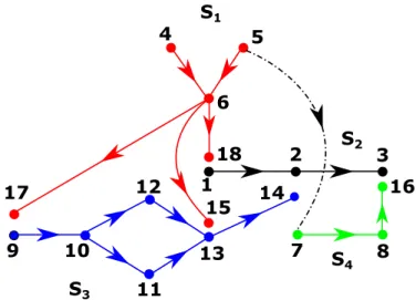
Engineers and system designers are under immense pressure to build systems robust and adequate enough to meet the ever increasing human demand and expectation. Unavoidably, the resulting systems are complex and highly interconnected, which iron-ically constitute a threat to their resilience and sustainability. The majority of the systems we interact with exist as multi-state interdependent systems. Two systems are interdependent if at least a pair of components (one from each system) are coupled by some phenomena, such that a malfunction of one aects the other. The coupling phe-nomenon could be proximity in space [23], functional dependence/interdependence [159], or both [158]. A water distribution network, where pumps and other electrical power-driven appliances rely on the reliability and performance of the power grid is a typical example.
The components of a system are normally prone to random failures arising from their intrinsic properties or induced failures stemming from targeted attacks [13], extreme environmental events [2], or erroneous human-system interactions. In interdependent systems, an undesirable glitch in one system could cascade and cause disruptions in coupled systems. The cascade could be fed back into the initiating system and the overall consequences may be catastrophic [23,63]. This was made clear by the massive blackout that struck Italy in September 2003, aecting the internet network in the process. In the same year, North America was hit by a 4-day blackout, aecting parts of USA and Canada [135]. To minimize the eects of failures, some interdependent systems are equipped with reconguration provisions. This normally entails transferring operation to another component, rerouting ow through alternative paths, or shutting down parts of the system. It is, therefore, vital to analyse the system's performance under the spectrum of possible vulnerability conditions, for adequate planning of defences [160].
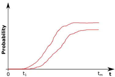
In general, the achievement of maximum overall system performance is desirable. However, in many applications, it is more important to recover the required system performance in the shortest possible time, after component failure. This is the case, for instance, in nuclear power plant risk assessment, where the time-dependent recovery probability of osite power is an important input to the overall safety of the plant [53]. Hence, system recovery time is not only a performance parameter, but a fundamental safety parameter, as well. Given the positive correlation between costs and resources (human, nancial, and material) required to maintain a system, under economic con-straints, there may not be sucient resources for a speedy recovery. Therefore, an informed and robust decision making process would dictate that the decision support tool used be capable of modelling the relevant realistic aspects of the system, including the possibility of limited recovery response.
Interdependencies
Inter-component Inter-system
Functional Induced
Cascading Events
Common-Cause Failures
Figure 2.1: Forms of interdependencies in engineering systems.
2.2.1 Forms of Interdependencies
Interdependencies in engineering systems are manifested at two levels: between com-ponents (inter-component), which can be functional or induced and between sys-tems/subsystems (inter-system). Functional dependencies are due to the topological and/or functional relationships between components. For instance, a motor-operated valve would not work if the electric motor controlling its actuator stopped due to a breaker failure. In this case, the valve is said to be functionally dependent on the breaker through the motor. Induced dependencies, on the other hand, are due to a state change in one component (the initiator) triggering a state change in another (the induced), such that even when the initiator is reinstated, the induced does not reinstate, unless manually made to do so. In the valve-motor-breaker example, for instance, the valve would resume its normal operation once the faulty breaker is replaced, highlighting the dichotomy between functional and induced dependencies. Functional dependencies are intrinsically accounted for by the innate attributes of the system reliability mod-elling and evaluation technique while induced dependencies require explicit modmod-elling. Induced dependencies are further divided into Common-Cause Failures (CCF) and cas-cading events, as illustrated in Figure 2.1.
Inter-system dependencies are due to functional or induced couplings between mul-tiple systems. Unlike standalone systems, functional dependencies in these systems may require explicit modelling. This is the case especially for components relying on mate-rial generated and transmitted by those of another system, under which condition the
reliability modelling technique used may prove inadequate. 2.2.1.1 Common-Cause Failures
Common-Cause Failures (CCF) are the simultaneous failure of multiple similar com-ponents due to the same root cause [103105]. Their origin is traceable to a coupling that normally is external to the system. Notable instances are shared manufacturing lines/materials, shared maintenance teams, shared environments, and human error. A group of components susceptible to the same CCF event is called a Common-Cause Group (CCG). An important point to note about Common-Cause Failures is that, on occurrence of the failure event, there is a probability associated with multiple compo-nent failure and that the aected compocompo-nents fail in the same mode. Consequently, the number of components involved in the event ranges from 1 to the total number of components in the CCG. CCF events may aect an entire system or only a few of its components. They have been shown (in [36], for instance) to decrease the reliabil-ity and performance of multi-component systems. They, therefore, must be given due consideration in system reliability evaluation, to minimise overestimation.
CCF modelling and quantication has always attracted keen interest from both researchers and practitioners of system reliability and safety engineering. A total of ve parametric models have been put forward to express the CCF probability associated with a CCG. The original model, the Basic Parameter Model (BPM), expresses the probability of a basic failure event involving a specic number of components. The other models, the β-factor model, the Multiple Greek Letter Model (MGL), the α -factor model, and the Binomial Failure Rate model, are mere reparameterizations of the BPM. Of these, the MGL and the α-factor models are the most widely used in system reliability and risk assessment. See Refs. [103, 104] for details on these models and their relationships.
Rasmuson and Kelly reviewed in their work [116], the basic concepts of modelling CCFs in reliability and risk studies. Rausand and Arnljot [117] proposed the square-root method, a simple bounding technique that estimates the eects of CCF on a system but which, however, lacks a strong mathematical foundation to support its application to practical systems. A robust Bayesian approach for quantifying the α-factor param-eters of a CCG in the presence of epistemic uncertainties has also been put forward by Troaes et al. [133]. Their approach, however, is limited to component-level relia-bility and, therefore, requires a second approach to obtain the system-level reliarelia-bility indices. For this, Fan's stochastic hybrid systems model [48], O'Connor's general cause-based methodology [106], or Ramirez-Marquez's reliability optimization approach [114], amongst others, would do, and only if the reliability analyst is willing to turn a blind eye to their respective drawbacks - these models are built on reliability evaluation tech-niques that do not segregate the topological from the probabilistic attributes of the
system. As such, they are computationally expensive for problems involving multiple reliability analysis of the same system. They also have yet to be applied to multi-state systems, as well as systems susceptible to both cascading and common-cause failures. 2.2.1.2 Cascading Failures
Cascading failures are those with the capacity to trigger the instantaneous failure of one or more components of a system. They can originate from a component or from a phenomenon outside the system boundary. The likelihood of the initiating event originating from within the system, distinguishes them from CCF. Another point of dichotomy is that the aected components do not necessarily have to be similar or fail in the same mode. In addition, at the occurrence of the initiating event, the probability of all the coupled components failing is unity, save for the case when they are in a state rendering them immune. A few prominent examples of initiating events external to the system are extreme environmental events, natural disasters, external shocks, erroneous human-system interactions, and terrorist acts.
Various models have been developed to study the eects of