East Tennessee State University
Digital Commons @ East
Tennessee State University
Electronic Theses and Dissertations Student Works
5-2013
A Comparison of Leading Database Storage
Engines in Support of Online Analytical Processing
in an Open Source Environment
Gabriel Tocci
East Tennessee State University
Follow this and additional works at:https://dc.etsu.edu/etd Part of theDatabases and Information Systems Commons
This Thesis - Open Access is brought to you for free and open access by the Student Works at Digital Commons @ East Tennessee State University. It has been accepted for inclusion in Electronic Theses and Dissertations by an authorized administrator of Digital Commons @ East Tennessee State University. For more information, please [email protected].
Recommended Citation
Tocci, Gabriel, "A Comparison of Leading Database Storage Engines in Support of Online Analytical Processing in an Open Source Environment" (2013).Electronic Theses and Dissertations.Paper 1111. https://dc.etsu.edu/etd/1111
A Comparison of Leading Database Storage Engines in Support of Online Analytical Processing in an Open Source Environment
_____________________
A thesis presented to
the faculty of the Department of Computer and Information Science East Tennessee State University
In partial fulfillment of the requirements for the degree
Master of Science in Computer and Information Science
_____________________
by Gabriel Tocci
May 2013
_____________________
Dr. Ronald Zucker, Chair Dr. Don Bailes Dr. Tony Pittarese
2 ABSTRACT
A Comparison of Leading Database Storage Engines in Support of Online Analytical Processing in an Open Source Environment
by Gabriel Tocci
Online Analytical Processing (OLAP) has become the de facto data analysis technology used in modern decision support systems. It has experienced tremendous growth, and is among the top priorities for enterprises. Open source systems have become an effective alternative to
proprietary systems in terms of cost and function. The purpose of the study was to investigate the performance of two leading database storage engines in an open source OLAP environment.
Despite recent upgrades in performance features for the InnoDB database engine, the MyISAM database engine is shown to outperform the InnoDB database engine under a standard
benchmark. This result was demonstrated in tests that included concurrent user sessions as well as asynchronous user sessions using data sets ranging from 6GB to 12GB. Although MyISAM outperformed InnoDB in all test performed, InnoDB provides ACID compliant transaction technologies are beneficial in a hybrid OLAP/OLTP system.
3 CONTENTS Page ABSTRACT ... 2 LIST OF TABLES ... 7 LIST OF FIGURES ... 8 Chapter 1. INTRODUCTION ... 10 2. BACKGROUND ... 14
2.1 The Open Source Software Development Model ... 14
2.2 Open Source Database Storage Engines ... 17
2.2.1 Storage Engine History... 17
2.2.2 MySql ... 18
2.2.2.1 MyISAM ... 19
2.2.2.2 InnoDB ... 19
2.3 Online Analytical Processing ... 20
2.3.1 Analytical and Transactional Processing Incompatibilities ... 20
2.3.2 Benefit to End Users ... 22
2.3.3 Multidimensional Data Model ... 23
2.3.4 OLAP Operations ... 24
4
2.3.5.1 ROLAP ... 25
2.3.5.2 MOLAP... 28
2.3.5.3 HOLAP ... 28
2.3.6 Data Homogenization ... 28
2.4 Open Source Online Analytical Processing Engines ... 29
2.4.1 Mondrian ... 29
2.4.2. Palo ... 30
2.4.3. Comparison... 30
2.5 Industry Standards ... 30
2.5.1 Java Database Connectivity ... 30
2.5.2 Multidimensional Expressions ... 31
2.4.3 Extensible Markup Language for Analysis ... 31
2.6 Online Analytical Processing Performance Benchmarks... 32
2.6.1 Analytical Processing Benchmark ... 32
2.6.2 TPC-DS ... 33
2.7 Summary ... 34
3. EXPERIMENTAL METHODS... 35
3.1 Motivation ... 35
3.2 Open Source Compliance ... 36
5
3.4 Online Analytical Processing Performance Benchmark ... 37
3.4.1 Benchmark Overview ... 37 3.4.2 Data Model ... 37 3.4.3 Database Population ... 38 3.4.4 Data Analysis... 39 3.4.5 Query Implementation ... 40 3.4.6. Performance Statistics ... 42 3.5 Server Configuration ... 43 4. RESULTS ... 45 4.1 Feature Summary ... 45 4.2 TPC-DS Benchmark Results ... 46
4.2.1 TPC-DS Power Test Statistics ... 46
4.2.2 TPC-DS Throughput Test Statistics ... 56
4.3 Scaled Data Size Summary ... 65
5. ANALYSIS ... 74
5.1 Qualitative Analysis ... 74
5.2 Quantitative Analysis ... 75
5.2.1 Power Test Performance Comparison ... 75
5.2.2 Throughput Test Performance Comparison ... 76
6
5.2.4 Scaled Data Set Test Performance Comparison ... 79
6. CONCLUSIONS... 82
6.1 Final Conclusions ... 82
6.2 Future Work ... 82
WORKS CITED ... 84
APPENDICES ... 90
Appendix A: Physical Representation of TPC-DS Relational Schema ... 90
Appendix B: Physical Representation of TPC-DS OLAP Schema ... 107
Appendix C: Cube Diagrams ... 118
Appendix D: Server Cofiguration ... 121
Appendix E: Jmeter Test Plan ... 124
Appendix F: TPC-DS Benchmark Results ... 135
Appendix G: TPC-DS Scaled Data Set Benchmark Results ... 157
7
LIST OF TABLES
Table Page
1. Open Source Definition Requirements ….………...… 16
2. TPC-DS Raw Table Size ……….……… 38
3. TPC-DS Queries ………....……….. 40
4. Feature Summary ……….……… 45
8
LIST OF FIGURES
Table Page
1. OLAP Server Architecture ……….. 22
2. Multidimensional Data Structure ……… 23
3. Consolidation Paths …….……… 24
4. Star Schema ….……….………...…… 26
5. Snowflake Schema ……….……….. 27
6. MDX Query Syntax ………. 31
7. XMLA Execute Request ……….. 32
8. Queries per Hour for Decision Support (QphDS) Formula ………. 43
9. Server Architecture ………..… 44
10.Power Test Query 1 Box Plot ……….. 47
11.Power Test Query 2 Box Plot ……….. 48
12.Power Test Query 3 Box Plot ……….. 49
13.Power Test Query 4 Box Plot ……….. 50
14.Power Test Query 5 Box Plot ……….. 51
15.Power Test Query 6 Box Plot ……….. 52
16.Power Test Query 7 Box Plot ……….. 53
17.Power Test Query 8 Box Plot ……….. 54
18.Power Test Query 9 Box Plot ……….. 55
19.Throughput Test Query 1 Box Plot ……….… 56
20.Throughput Test Query 2 Box Plot ………. 57
9
22.Throughput Test Query 4 Box Plot ……….……….… 59
23.Throughput Test Query 5 Box Plot ……….……….… 60
24.Throughput Test Query 6 Box Plot ……….……….… 61
25.Throughput Test Query 7 Box Plot ……….……….… 62
26.Throughput Test Query 8 Box Plot ……….……….… 63
27.Throughput Test Query 9 Box Plot ……….……….… 64
28.Throughput Test Query 1 Box Plot ……….……….… 66
29.Throughput Test Query 2 Box Plot ……….……….… 67
30.Throughput Test Query 5 Box Plot ……….……….… 68
31.Throughput Test Query 7 Box Plot ……….……….… 70
32.Throughput Test Query 8 Box Plot ……….……….… 71
33.Throughput Test Query 9 Box Plot ……….………. 72
34.Power Test Performance Comparison ……….……… 76
35.Throughput Test Performance Comparison ……….……… 77
36.Queries per Hour for Decision Support (QphDS) Formula ……….……… 78
37.Queries per Hour for Decision Support (QphDS) Comparison ………….……….. 78
10 CHAPTER 1 INTRODUCTION
Online Analytical Processing (OLAP) systems enable business leaders and executives to analyze large amounts of data quickly and interactively. This ability provides insight into the business in a manner understandable to the user to support decision making. This work analyzed the performance of leading database storage engines in support of OLAP in an open source environment under a standard benchmark defined by the Transaction Processing Council [1].
OLAP has become the de facto data analysis technology used in modern decision support systems, commonly referred to as Business Intelligence (BI) or Executive Information Systems (EIS). Decision support systems have experienced tremendous growth and are among the top priorities for enterprises [2]. All principal DBMS (e.g. Oracle, Microsoft, and IBM) vendors now have offerings in data warehousing and OLAP technologies [3].
BI Systems were first proposed in 1958 by H.P. Luhn [4]. Although the specific technologies proposed to be used by Luhn are no longer relevant, many of the theoretical characteristics proposed in 1958 remain [4]. Effective decision support systems leverage a wealth of business data from numerous touch points and translate it into tangible and lucrative results [5]. BI is an information technology (IT) system, “that allows organizations to access, analyze, and share information across the organization … BI provides employees with
information to make better decisions, and can be used in environments ranging from workgroups of 20 users to enterprise deployments exceeding 20,000.” [6]. BI gives executives and key decision makers the ability to see business processes with a high level of transparency [6].
OLAP was developed to solve the significant technical challenges in efficiently analyzing large amounts of data [7]. This solution is facilitated through storage, retrieval, and analysis of
11
enterprise data in its natural, multidimensional perspective. This multidimensional data model is the structural difference between OLAP and its relational counterpart, Online Transactional Processing (OLTP) systems, that enables efficient analytical processing.
Open source software is developed under a license that is based on the idea of a free exchange of technical information. Sharing of technical specifications for software (source code) has proven to be an excellent development model because it grants every user the freedom to change the source code [8]. Although not a universal agreement, recent studies have been
released that provide quantitative data proving open source software is a reasonable, and in some cases a superior, software solution [9, 10]. Open source BI is out of the innovation stage and has progressed from almost nothing a decade ago, into the mainstream with community and
commercially supported projects [11].
This work investigates the performance of leading database storage engines developed using the open source model in an OLAP environment. The following steps are conducted:
A brief analysis to confirm the storage engines are in compliance with open source requirements.
A technical comparison of the storage engines, and identification of fundamental components that support OLAP.
A performance benchmark comparison of the storage engines based on the Decision Support Benchmark (TPC-DS), as defined by the Transaction Processing Council.
Two additional TPC-DS benchmark tests, executed on scaled data sets to determine if execution times scale in proportion to data set size.
12
Previous research exists showing strong development and maturity in open source BI user tools, but not the underlying engines [12]. Recent benchmarks have been performed that explore the leading open source database engines, and one, InnoDB, has undergone extensive updates in its most recent version [13, 14, 15]. Recent data on the performance of the leading open source database engines in support of OLAP has not been published with respect to a standard
benchmark or the recent updates to InnoDB. The work presented here seeks to address this gap in the literature and determine the performance of the leading open source database storage engines in support of OLAP. This work is timely due to the strained global economic situation, the emergence of the TPC-DS as an industry standard OLAP benchmark, and the recent release of updates to the InnoDB storage engine [14, 16].
During a strained economic situation it is generally acceptable to simply maintain market share and profitability. With BI, organizations can actually improve market share and
profitability [6]. Open source BI has become an effective alternative to proprietary systems [11]. Although the top reason for open source adoption is cost savings, reduced vendor dependence and ease of integration follow closely behind [11]. BI leverages existing Information Technology (IT) infrastructure, such as Enterprise Resource Planning (ERP) and Customer Relationship Management (CRM), by analyzing data previously stored in these existing systems without significant investment [6]. “Business enterprises prosper or fail according to the sophistication and speed of their information systems, and their ability to analyze and synthesize information using those systems.” [7].
The remainder of this work includes chapters organized as follows: Chapter Two provides background information and resources detailing the topics examined in this research. Chapter Three introduces the experimental methods used to compare of these engines, and
13
Chapter Four presents the results of these experiments. Chapter Five summarizes and discusses the data presented in Chapter Four. Chapter Six explains the significance these results conclude, as well as suggestions for further research avenues on this subject matter.
14 CHAPTER 2 BACKGROUND
This chapter includes background information and resources detailing the topics examined in this research. Topics include open source software development specifications, a survey of the leading open source database management system and its storage engine
technologies, OLAP architectures, OLAP standards, OLAP benchmarking, and open source OLAP products.
2.1 The Open Source Software Development Model
Open source is a philosophy based on the idea of a free exchange of technical
information. The idea dates back long before computers, and can be seen as far back as 1911 when Henry Ford won a challenge to the patent of George B. Sheldon [17]. Sheldon attempted to monopolize the automobile industry by patenting the gasoline engine. The ruling in this case created the Motor Vehicle Manufacturers Association, which freely shared technical information about patented automobile technology through licensing agreements [17]. Licensing agreements for openly shared technology is the mechanism that supports open source software.
Sharing of technical specifications for software, or source code, has proven to be an excellent development model because it grants every user the freedom to change the source code [8]. Many of the leading software products available today, such as Linux, Apache, PGP, Perl, and Python, have been developed using the open source development model.
In April 1998, the “Open Source Summit” brought together the leaders of many of the most important open source projects to discuss the benefits, problems, and raise awareness of open source software development. The development model was originally referred to as
15
freeware or source ware, but many developers of such products were not happy with that name. A result of the session was the establishment of the official name: open source [8].
The Open Source Initiative (OSI), a California based non-profit organization, is steward for the Open Source Definition (OSD). To bear the term "open source", a product must be in compliance with ten requirements of the OSD, listed in Table 1 [18].
Table 1. Open Source Definition Requirements [19]
1. Free Redistribution The license shall not restrict any party from selling or giving away the software as a component of an aggregate software distribution containing programs from several different sources. The license shall not require a royalty or other fee for such sale.
2. Source Code The program must include source code, and must allow
distribution in source code as well as compiled form. Where some form of a product is not distributed with source code, there must be a well-publicized means of obtaining the source code for no more than a reasonable reproduction cost preferably, downloading via the Internet without charge. The source code must be the preferred form in which a programmer would modify the program. Deliberately obfuscated source code is not allowed. Intermediate forms such as the output of a preprocessor or translator are not allowed.
3. Derived Works The license must allow modifications and derived works, and must allow them to be distributed under the same terms as the license of the original software.
4. Integrity of The Author's Source Code
The license may restrict source-code from being distributed in modified form only if the license allows the distribution of "patch files" with the source code for the purpose of modifying the program at build time. The license must explicitly permit distribution of software built from modified source code. The license may require derived works to carry a different name or version number from the original software.
5. No Discrimination Against Persons or Groups
The license must not discriminate against any person or group of persons.
16 ( Table 1. continued )
6. No Discrimination Against Fields of Endeavor
The license must not restrict anyone from making use of the program in a specific field of endeavor. For example, it may not restrict the program from being used in a business, or from being used for genetic research.
7. Distribution of License
The rights attached to the program must apply to all to whom the program is redistributed without the need for execution of an additional license by those parties.
8. License Must Not Be Specific to a Product
The rights attached to the program must not depend on the program's being part of a particular software distribution. If the program is extracted from that distribution and used or distributed within the terms of the program's license, all parties to whom the program is redistributed should have the same rights as those that are granted in conjunction with the original software distribution. 9. License Must Not
Restrict Other Software
The license must not place restrictions on other software that is distributed along with the licensed software. For example, the license must not insist that all other programs distributed on the same medium must be open-source software.
10. License Must Be Technology-Neutral
No provision of the license may be predicated on any individual technology or style of interface.
There are many different variations of open source software licenses, models, and governance structures [18]. “Each of these elements has profound implications for the type and size of the resulting community, the market penetration and distribution, the ability to recombine with other open source projects, the resistance to unintended or anticipated forks, and more.” [18]. Open source software is commonly differentiated by the type of license agreement to which it adheres.
According to OSI, the most commonly used open source licenses with a strong community are The Apache License 2.0, The New and Simplified BSD licenses, The GNU General Public License (GPL), The GNU Library or "Lesser" General Public License (LGPL),
17
The MIT license, The Mozilla Public License 1.1 (MPL), and The Common Development and Distribution License. The OSI has sixty-five open source licenses approved for use [20].
The primary driving factor attributed to the popularity and adoption of open source database software in business today is cost savings. As the CEO of RightNow, a large CRM provider, has observed:
"Using MySQL and other open source technologies, RightNow has built an enterprise-class CRM application hosting environment that supports over 3,000 deployments for some of the world's largest organizations…Our systems have facilitated over 1 billion customer
interactions on behalf of our clients while maintaining reliability at or above 99.97 percent. Money spent on proprietary databases, when there is a viable open source alternative, is money wasted." [21].
2.2 Open Source Database Storage Engines
A database storage engine is the main software component of a database management system (DBMS). It facilitates the underlying create, read, update, and delete (CRUD) operations performed on the physical data [22].
2.2.1 Storage Engine History
The DBMS examined in this study, MySQL, is based on relational mathematics. This relational model for databases was proposed by E.F. Codd in 1970 [23]. His paper is considered a landmark because it was the first proposal of a disconnection between the logical organization of a database, or schema, from the physical data storage. This has been the standard DMBS architecture ever since, because it separates user operations from the changes in data representation caused by growth. Codd also introduced a normal form for managing the
18
collection of relationships, as well as operations on relations. This work shaped the modern DBMS, and is the technology used in the open source OLAP system examined in this study [23]. 2.2.2 MySql
For over twelve years, MySQL has been the leading open source DBMS, and is the “M” in the popular open source LAMP server stack (Linux, Apache, MySQL, PHP/Perl/Python). Many large, successful companies rely on MySQL to manage their data-driven applications, including Google, Yahoo, NY Times, Cox Communications, The Associated Press, Symantec, Alcatel, Nokia, Nortel, Cisco, and Zappos [24]. MySQL is downloaded over 65,000 times daily and by 2008, MySQL was estimated to have a 50% market share of all database installations with over 16000 paying customers [25]. In terms of open source downloads, MySQL trails only the Mozilla Firefox Browser [24]. The leading news website, Weather.com, switched to MySQL from an unnamed proprietary database, and stated a, “30 percent increased capacity and 50 percent decreased cost” [26].
Several different storage engines are supported by MySQL Server. These various storage engines provide different capabilities to database administrators (DBA’s) and software
developers.
Since version 5.1, MySQL Server has featured a pluggable storage engine architecture. This architecture enables multiple storage engines to be enabled in a single database instance. This modular architecture enables a DBA to select a specialized storage engine for a particular application, such as transaction processing, data warehousing, Business Intelligence, or high availability, based on the needs of the system [27].
The MySQL server architecture separates software applications from the underlying storage engine via Connector APIs and service layers. Software developers interact with MySQL
19
through these Connector APIs and service layers as well. If changes to the requirements create the need for a different storage engine, changes to the software under development are not required [27].
Although MySQL offers database designers and administrators many choices when it comes to choosing a specialized storage engine, the MyISAM and InnoDB storage engines are the most widely used [15]. InnoDB became the default storage engine in MySQL version 5.5. In all previous versions, MyISAM was the default storage engine [14].
2.2.2.1 MyISAM. MyISAM is not a transaction-safe storage engine. It is used in situations that value high levels of query throughput over referential-integrity and muti-user concurrency. MyISAM has been identified as a good general engine for data marts and traditional data warehouses. Its primary advantage on query performance is its lack of referential-integrity constraints. Other advantageous features of MyISAM include full-text indexing and decreased database design effort. This simpler storage structure reduces the amount of required server resources on large queries [24, 28, 29]. The primary disadvantage of MyISAM on query performance is its dependence on table-level locking [28, 29].
2.2.2.2 InnoDB. The ACID model sets four requirements that a DBMS must achieve for compliance: atomicity, consistency, isolation and durability. InnoDB is a transaction safe, ACID compliant, MySQL storage engine, recommended for situations where query performance is not the only priority. InnoDB has the popular database transaction features of commit and rollback, as well as crash-recovery capabilities to protect data. InnoDB’s primary advantage for query performance is non-locking reads. To reduce disk I/O for common queries, it stores user data in clustered indexes. MySQL claims that, “InnoDB’s CPU efficiency is not matched by any other
20
disk-based relational database engine”. The primary disadvantage of InnoDB on query performance is its referential-integrity constraints [28, 29].
In Version 5.5, MySQL made changes to the InnoDB Input Output (I/O) subsystem. These changes are designed to increase the I/O performance, and configurability [14].
In previous versions, InnoDB underutilized server capabilities by prefetching disk blocks and flushing dirty pages with only one background thread. Pages are the basic internal structure used to organize data in the database files. Dirty pages are modified, uncommitted pages, still in the buffer pool [30]. This version enables the utilization of multiple threads [31].
The number of background threads used for page I/O is exposed via system variables, and the default setting is four. Also, the number of I/O operations per second (IOPS) is now an exposed system variable. In previous versions, the IOPS setting was a compile-time parameter. The IOPS rate is a limit that prevents background I/O from exhausting server capability. A higher I/O rate enables the server to process a higher rate of page changes in the buffer pool. Many modern systems can exceed the previous default value, which would unnecessarily restrict I/O utilization [31]. These changes were made to increase system performance and
configurability.
2.3 Online Analytical Processing 2.3.1 Analytical and Transactional Processing Incompatibilities
In 1993, E. Codd, S. Codd, and C. Salley, published a paper that describes the need for a new category of database processing called Online Analytical Processing (OLAP) [7]. OLAP has become the de facto data analysis technology used in modern decision support systems,
21
The name OLAP differentiates this new type of analytical database from its transactional counterpart, the Online Transaction Processing (OLTP) database. OLTP databases are the traditional, transaction based databases used to store day to day business data in organizations throughout the world. Transactional databases are structured for short, repetitive, isolated, atomic transactions. Transactions provide an accurate and powerful solution for creating, retrieving, updating, and deleting enterprise data [3]. OLTP provides users with up to date data at a high level of detail, where analytical applications provide summarized, historical, consolidated data, more appropriate for business analysts [5].
Key performance metrics for OLTP databases include a minimization of concurrency conflicts, consistency, recoverability, and transaction throughput. OLAP performance metrics key on query intensive workloads that are mostly ad-hoc and complex, accessing millions of records containing a lot of scans, joins, and aggregates [3].
Efficient OLAP systems must be implemented as entirely separate databases from OLTP systems because the physical design required for adequate performance of each is incompatible. To address the shortcomings of databases that existed in the late 1960’s, such as being difficult to maintain, secure, and understand, OLTP databases were developed using relational
mathematic theory [7]. Relational databases depend on the Entity-Relationship (ER) data model, which presents significant technical challenges in analyzing large amounts of data [32]. The ER data model reflects a strong emphasis on structure, which is excellent for transactional databases, but neglects architecture for analysis. OLTP databases fail to provide an effective solution for data analysis because it lacks the ability to consolidate, view, and analyze data from multiple perspectives, also referred to as dimensions [7].
22
Figure 1. OLAP Server Architecture
2.3.2 Benefit to End Users
Not only has the amount of data stored by organizations experienced a dramatic increase, “The number of individuals within an organization who have a need to perform more
sophisticated analysis is growing.” [7]. OLAP databases provide many benefits to end users. Data in an OLAP database is arranged by business areas, and these business areas are uniquely defined by the data requirements of an individual company. Once the database administrator defines the business areas, end users have access to their own data organized in familiar fashion.
OLAP front end applications do not require end users, such as business analysts,
operational managers, and executives, to learn the query languages. This empowers the end users to satisfy their own data requirements, and avoid reliance on Information Technology (IT) staff [33]. These applications also provide end users with the ability to manipulate data aggregations and formats to perfect their reports.
23 2.3.3 Multidimensional Data Model
Businesses naturally view themselves from multiple perspectives, such as time, location, and sales. OLAP facilitates this complex, multi-perspective analysis via complex data models, access methods, and implementation methods [3].
The objects being analyzed in this multi-perspective data model are referred to as measures, or facts. The perspectives for which the measure is viewed are referred to as
dimensions. A dimensions scope is defined by its attributes, and the most commonly analyzed dimension is time, due to its significance in trend analysis [3]. The simultaneous analysis of measures along multiple dimensions is referred to as multidimensional data analysis [7]. Each unique set of dimensions and measures is referred to as a multidimensional cube.
Figure 2. Multidimensional Data Structure
The historical nature of OLAP systems require summarized data for users to analyze. Data consolidation is the process of summarizing large amounts of data into single blocks of useful knowledge [7]. Hierarchies give OLAP engines a structure to effectively consolidate otherwise flat dimensions. A strong support for hierarchies is the principal conceptual feature that distinguishes the multidimensional and relational data models. The attributes of a dimension
24
related along hierarchical relationships, or consolidation paths, are shown in Figure 3 [3]. There are substantial differences in the hierarchy implementation methods among OLAP products [34].
Figure 3. Consolidation Paths 2.3.4 OLAP Operations
Before multidimensional data analysis, data analysts were unable to efficiently change between data dimensions and aggregate levels of detail. Data analysts interactively navigate a cube using the OLAP operations rotate and slice and dice [35]. OLAP facilitates these operations efficiently using vector arithmetic [36].
Changing levels of consolidation is referred to as drilling down, or rolling up. A drill down is the downward traversal of the hierarchy from the most summarized level to the most detailed level [5]. A roll up, or aggregation, refers to the opposite, upward hierarchy traversal. Rotation, also referred to as pivoting, is changing the dimensional orientation of a measure [35]. A slice is a subset of a measure, where a specified value corresponds to an attribute of a
dimension [35]. Slicing and dicing are the user initiated processes associated with navigating through slices using rotation, drill down and drill up [35].
OLAP operations frequently span multiple consolidation paths and dimensions [7]. These consolidations commonly involve complex statistical equations and computations such as
25
moving averages, percentage change between time periods, and inter-dimensional comparisons, such as sales and budget [5].
The complex processing involved with multidimensional data analysis and these consolidation operations is extremely cumbersome on database systems. Optimizing these processes was the primary motivation behind the development of OLAP [7].
2.3.5 OLAP Engine Architectures
2.3.5.1 ROLAP. Relational Online Analytical Processing (ROLAP) Engines use middleware between back end relational databases and front end OLAP client tools. The middleware generates indices, views, and multi-statement SQL for the relational database [5].
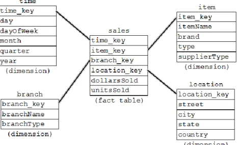
ROLAP uses a rich multidimensional metadata model called a star schema to implement OLAP on relational data stores. Star schemas implement a table for each multidimensional measure, referred to as a fact table. Dimensions are also implemented as tables with the columns representing its attributes. The rows of the fact table form foreign key relationships to the
dimension tables, as illustrated in Figure 4. Breaking the normalization rules that that preserve the accuracy of relational schemas by star schemas is acceptable because OLAP databases are not required to be instantaneously accurate [7].
26
Figure 4. Star Schema
Although computing joins between fact tables and dimension tables are more efficient than arbitrary relations, intrinsic mismatches between the relational model and the
multidimensional model can create performance bottlenecks [5]. As an effort to offset
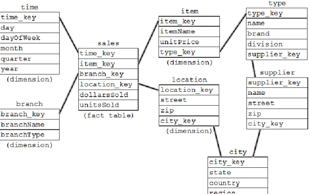
performance bottlenecks, ROLAP engines implement a multitude of optimization techniques. Snowflake schemas are used to improve storage utilization via dimension table normalization [5]. Normalizing the dimension tables creates explicitly represented attribute hierarchies that eliminate redundancy [37]. Fact constellation schemas are snowflake schemas where multiple fact tables share dimension tables to improve storage utilization, as illustrated in Figure 5 [5]. Snowflake and fact constellation schemas increase query complexity and reduce query performance [37].
27
Figure 5. Snowflake Schema
If maximum storage utilization is not a requirement, join indices and materialized views can increase processing performance for complex queries. Join indices index key relationships between fact and dimension tables, and materialized views store commonly aggregated data. Join indices are effective for data selective queries, but ineffective for data intensive queries because they often require entire relations to be scanned sequentially. The difficulties in implementing join indices and materialized views are proper identification, effective use, and proper updating [5].
ROLAP vendors implement star transformations to improve star schema query
performance. Rather than computing a Cartesian product of the dimension tables, this process combines bitmap indexes on individual fact table columns. This improves performance in cases with sparse data sets or a large number of dimensions [37].
28
2.3.5.2 MOLAP. Multidimensional Online Analytical Processing (MOLAP) Engines implement OLAP in its quintessential form, through direct mapping on a multidimensional storage layer [3]. The disadvantage of MOLAP is inefficient storage utilization for sparse data sets [5]. It is addressed through extensive data compression and two level storage representations [5]. Using two level data representations, a technique acquired from statistical databases, uses elements of a dense data set to index smaller sparse data sets [5].
2.3.5.3 HOLAP. Hybrid Online Analytical Processing (HOLAP) combines features of ROLAP and MOLAP. HOLAP engines divide complex queries into sub queries based on data set density. Queries spanning dense data sets are processed by MOLAP subsystems, and queries spanning sparse data sets are processed by ROLAP subsystems. The result sets are then
combined and presented to the end user [5].
HOLAP systems store the majority of the data in relational databases to avoid problems attributed to sparsity. The multidimensional part of the system stores only the frequently accessed data. If the multidimensional data cannot answer the query, the system then transparently accesses the relational part of the system [38].
2.3.6 Data Homogenization. Data homogenization is the process of processing data from diverse physical data representations, including flat files, data feeds, and databases, into a logically consistent data structure and central location for analysis and reporting [7]. These diverse sources may contain data of varying quality, codes, and formats, which must be reconciled prior to data load [3]. This process is often referred to as Extract Transfer Load (ETL), and is a prerequisite to OLAP.
29
Approximate query processing, sometimes referred to as Approximate Query Answering (AQUA) is the process of answering queries using small, precompiled data samples, or synopsis to answer arbitrary aggregate queries [5, 39]. This part of data homogenization is intended to improve query processing performance.
Building an effective data warehouse schema can take years due to complex business modeling. To expedite this process, businesses often opt to create departmental data marts. Disjoint analysis and analysis synthesis are unfavorable facets of data mart implementation [5].
2.4 Open Source Online Analytical Processing Engines
The availability of production ready open source OLAP engines is limited, and only two were found. Mondrian is a ROLAP server, and Palo is a memory-based MOLAP server. The Mondrian OLAP engine has become the de facto OLAP engine for open source solutions [40]. It is not only included in the Pentaho BI suite, but also in other open source BI suites [12].
2.4.1 Mondrian
Mondrian began as an independent open source project in 2002 [12]. In 2005, Mondrian became a part of Pentaho's BI package. The most recent version of Mondrian is 3.3 (2012), is released under the Common Public License (CPL). Mondrian is a Java application, so it can run on platform with a Java Runtime Environment (JRE). It also uses Java Database Connectivity (JDBC), which can be integrated with most modern DBMSs. The Mondrian documentation consists of public facing web pages that total close to 200 pages of printed text. The Mondrian user forums are used actively [12].
The Mondrian project was involved in the standardization of olap4j, which is a common Java application programming interface (API) for OLAP servers. Olap4j is the preferred
30
MDX queries, and cube schemas are specified in XML. Mondrian is scalable to large data sets, and is limited only by the underlying DBMS because it delegates aggregation to the DBMS [12]. 2.4.2. Palo
Palo is a MOLAP server developed by Jedox AG [12]. It has a version released under the GPL, however this version has limited functionality. Documentation exists, but costs €29.50. Version 2.5 was released in early July 2008. Data sets are loaded into memory, thus data sets a limited to server memory allocation. Proprietary programming interfaces are required to
communicate with Palo. There is also a free, but closed-source client add-in for Microsoft Excel. This Excel add-in is the primary client user interface [12].
2.4.3. Comparison
Due to the differences in architecture, standards compliance, and open source features, Mondrian was chosen to implement this experiment.
2.5 Industry Standards 2.5.1 Java Database Connectivity
The Java Database Connectivity (JDBC) framework gives Java application developers a common database access method that is platform agnostic. The classes of the JDBC API are open source and available from the Sun website (http://docs.oracle.com/javase/7/docs/api/).
JDBC builds on the existing Open Database Connectivity (ODBC) standard, increasing the abstraction level. ODBC is a standard that consolidated the commonality between DBMS’s. JDBC-ODBC bridges exists to enable allow Java programs to connect to existing ODBC-enabled database software [42].
31 2.5.2 Multidimensional Expressions
Multidimensional Expressions (MDX) is the de facto query language for
multidimensional data. It was released in 1998 by Microsoft as the language component of the OLE DB for OLAP [43].
SELECT [<axis_specification>
[, <axis_specification>...]] FROM [<cube_specification>]
[WHERE [<slicer_specification>]]
Figure 6. MDX Query Syntax [44]
At first glance, MDX syntax in figure 6 appears similar to the Structured Query Language (SQL) traditionally used with relational databases. However, MDX is a completely new language with its own combinations of identifiers, expressions, operators, functions, comments, and keywords [44]. Translate MDX queries into traditional SQL queries would require synthesis of large SQL expressions for very simple MDX expressions [43].
2.4.3 Extensible Markup Language for Analysis
The Extensible Markup Language for Analysis (XMLA) is the standard API for data interaction between OLAP Servers and Clients, and is illustrated in figure 7 [45]. The
communication of data is implemented using the Hypertext Transfer Protocol (HTTP), Simple Object Access Protocol (SOAP), and Extensible Markup Language (XML) web standards. Using these web standards allow for development of hardware, platform, and location independent applications capable of implementing thin client architecture [45].
32 <Execute xmlns="urn:schemas-microsoft-com:xml-analysis" SOAP-ENV:encodingStyle= "http://schemas.xmlsoap.org/soap/encoding/"> <Command> <Statement>
select [Measures].members on Columns from Sales </Statement> <Command> <Properties> <PropertyList> <DataSourceInfo> Provider=Essbase;Data Source=local; </DataSourceInfo> <Catalog>Foodmart 2000</Catalog> <Format>Multidimensional</Format> <AxisFormat>ClusterFormat</AxisFormat> </PropertyList> </Properties> </Execute> </SOAP-ENV:Body> </SOAP-ENV:Envelope>
Figure 7. XMLA Execute Request [41]
2.6 Online Analytical Processing Performance Benchmarks 2.6.1 Analytical Processing Benchmark
The OLAP Council was an organization established to advocate the advancement of OLAP technology. “The mission of the OLAP Council is to educate the market about OLAP technology, provide common definitions, sponsor industry research and help position OLAP technology within a broader IT architecture”. The OLAP council also worked to establish standard OLAP terminology, interoperability guidelines, and the first analytical benchmark, the Analytical Processing Benchmark (APB-1) [35].
The APB-1 has been succeeded by the Decision Support Benchmark (TPC-DS) developed by the Transaction Processing Performance Council.
33 2.6.2 TPC-DS
For the last fifteen years, the TPC-D benchmark, and its successor TPC-H, have been used by industry and the research community to evaluate DSS performance. The Transaction Processing Performance Council recognized a paradigm shift in the industry and developed this TPC-DS benchmark. TPC-DS is now the industry standard DSS benchmark [16].
TPC-DS measures query throughput under a complex, controlled, multi-user workload for a given system under test (SUT), which includes server hardware, operating system, and database configuration. It is used by vendors to demonstrate system capabilities, by customers in purchasing software and servers, and by the research community for optimization development [46]. The database schema, data population, queries, and implementation rules are designed to broadly represent modern decision support systems and provide highly comparable, controlled, vendor-neutral, and repeatable tasks [46]. TPC-DS tests the upper boundaries of system
performance by examining a large volume of data and answering real world business questions by executing queries of various complexities [47].
The schema, an aggregate of multiple star schemas, models the decision support functions of a typical multichannel retail product supplier contains essential business
information, such as detailed customer, order, and product data in store, catalog, and internet channels [16]. The benchmark data generation utility uses real world data with common data skew where possible, such as seasonal sales and frequent names. A retail model helps readers relate the components of the benchmark intuitively [1].
The TPC-DS workload could be used to describe any retail supplier using BI to address complex business problems. The queries analyze and convert store, web and catalog sales channels operational facts into business intelligence using a variety of access patterns, query
34
phrasings, operators, and answer set constraints [16]. An intense query workload is necessary to preserve a realistic context [1].
2.7 Summary
This chapter included background information and resources detailing the topics examined in this thesis. Topics include open source software development specifications, a survey of the leading open source database management system and its storage engine technologies, OLAP architectures, OLAP standards, OLAP benchmarking, and open source OLAP products.
35 CHAPTER 3
EXPERIMENTAL METHODS 3.1 Motivation
As stated previously, this work investigated the performance of leading database storage engines in support of Online Analytical Processing (OLAP) in an open source environment. OLAP has become the de facto data analysis technology used in modern decision support systems, commonly referred to as Business Intelligence (BI) or Executive Information Systems (EIS). Decision support systems have experienced tremendous growth and are among the top priorities for enterprises [2]. All principal DBMS (e.g. Oracle, Microsoft, and IBM) vendors now have offerings in the data warehousing and OLAP technologies [3].
This work investigated the performance of leading database storage engines for OLAP developed using the open source model using the following steps:
A brief analysis to confirm the storage engines are in compliance with open source requirements.
A technical comparison of the storage engines, and identification of fundamental components that support OLAP.
A complete performance benchmark comparison of the storage engines based on the Decision Support Benchmark (TPC-DS), as defined by the Transaction Processing Council.
Two additional TPC-DS benchmark tests, executed on scaled data sets to determine if execution times scale in proportion to data set size.
Previous research has been performed that surveys open source BI tools [12]. Recent benchmarks have been performed that explore the leading open source database engines, and
36
one, InnoDB, has undergone extensive updates in its most recent version [13, 14, 15]. Recent data on the performance of the leading open source database engines in support of OLAP has not been published with respect to a standard benchmark, or the recent updates to InnoDB. The work described here has sought to address this gap in the literature and determine the performance of the leading open source database storage engines in support of OLAP. This work is timely due to the strained global economic situation, the emergence of the TPC-DS as an industry standard OLAP benchmark, and the recent release of updates to the InnoDB storage engine [14, 16].
During a strained economic situation it is generally acceptable to simply maintain market share and profitability, but with BI, organizations can actually increase these metrics [6]. Open source BI has become an effective alternative to proprietary systems in terms of cost and function [11]. The top reason for adoption is still cost savings, although reduced vendor dependence and ease of integration followed closely behind [11]. BI leverages existing Information Technology (IT) infrastructure, such as Enterprise Resource Planning (ERP) and Customer Relationship Management (CRM), by analyzing data previously stored in these existing systems without significant investment [6]. “Business enterprises prosper or fail according to the sophistication and speed of their information systems, and their ability to analyze and synthesize information using those systems.” [7].
3.2 Open Source Compliance
The database engines in this study were examined to determine if they are in compliance with ten requirements of the OSD, as this research attempted to assist the adoption of open source database software only. Storage engines included in this research must be released with one of the sixty-five open source licenses approved for use by the OSI.
37
3.3 Feature Comparison
The storage engines in this study were examined to identify fundamental database components and technologies. The differences in these components and technologies have brought to bear declarative performance differences.
3.4 Online Analytical Processing Performance Benchmark 3.4.1 Benchmark Overview
TPC-DS measures query throughput under a complex, controlled, multi-user workload for a given system under test (SUT), which includes server hardware, operating system, and database configuration. It is used by vendors to demonstrate system capabilities, by customers in purchasing software and servers, and by the research community for optimization development [46]. The database schema, data population, queries, and implementation rules are designed to broadly represent modern decision support systems, and provide highly comparable, controlled, vendor-neutral, and repeatable tasks [46].
3.4.2 Data Model
The schema, an aggregate of multiple star schemas, models the decision support functions of a typical multichannel retail product supplier. It contains essential business information, such as detailed customer, order, and product data in store, catalog, and internet channels [16]. The benchmark data generation utility uses real world data with common data skew where possible, such as seasonal sales and frequent names. This retail model helps readers relate the components of the benchmark intuitively [1].
The TPC-DS star schemas consist of seven fact and seven dimension tables. The fact tables include a pair of fact tables, sales and returns, for each of the three sales channels. The remaining fact table models product inventory. Each fact table has a correlated cube definition.
38
The seven dimensions are item, date, store, customer, customer address, customer demographics, household demographics, and promotion. The seven dimension tables are used across the
multiple cubes, and each contain a single column surrogate key, which is used to join the fact tables [1].
A detailed definition of the schemas can be found in the appendices. Appendix A
contains the relational schema, appendix B contains the multidimensional schema, and appendix C contains the cube diagrams.
3.4.3 Database Population
The TPC-DS specification mandates the supplied data generator, dsgen, be used to generate data for population of the SUT database. dsgen source code is included as part of the electronically downloadable portion of the specification, and benchmark implementers are permitted to modify dsgen [1]. However, this research did not require dsgen modification.
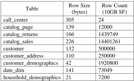
The specification defines scale factor (SF), which determines the approximate raw size of the data produced by dsgen [1]. This research used an initial SF of 10GB, which creates 12GB of raw data, and is displayed in table 2. In order to realistically scale the benchmark, the fact tables were scaled to create raw data sets of 9GB and 6GB. Dimensions tables were not scaled [46].
Table 2. TPC-DS Raw Table Size
Table Row Size
(bytes) Row Count (10GB SF) call_center 305 24 catalog_page 139 12000 catalog_returns 166 1439749 catalog_sales 226 14401261 customer 132 500000 customer_address 110 250000 customer_demographics 42 1920800 date_dim 141 73049 household_demographics 21 7200
39 ( Table 2. continued ) income_band 16 20 inventory 16 133110000 item 281 102000 promotions 124 500 reason 38 45 ship_mode 56 20 store 263 102 store_returns 134 2875432 store_sales 164 28800991 time_dim 59 86400 warehouse 117 10 web_page 96 200 web_returns 162 719217 web_sales 226 7197566 web_site 292 42 3.4.4 Data Analysis
The TPC-DS workload could be used to describe any retail supplier using BI to address complex business problems. The queries analyzed and converted the store, web and catalog sales channels operational facts into business intelligence using a variety of access patterns, query phrasings, operators, and answer set constraints [16]. An intense query workload was necessary to preserve a realistic context [1].
Although a modern DSS should support users with diverse needs such as reporting, ad-hoc, iterative OLAP, and data mining, this research is focused on OLAP performance. The OLAP queries implemented in this research were constructed to analyze large sets of business data, answer specific business questions, and determine meaningful trends. Due to the nature of changing business environments and diverse user needs, this research can only provide DBAs a limited degree of fore knowledge for performance planning [1].
40 3.4.5 Query Implementation
The query streams were implemented using a scenario-based user session. Each session contained a query sequence with each query leading to another. This model allows the
benchmark to capture important aspects of the complex, iterative nature of OLAP queries [1]. Each user session contained an identical set of queries, implemented as a JMeter user thread.
Apache JMeter was used to drive all testing and data collection. JMeter is an open source Java client application designed to load test functional behavior and measure system
performance under a concurrent load [48]. JMeter test plans detail the steps executed by JMeter. The complete TPC-DS JMeter test plan implemented for this research can be found in appendix E. Table 3 describes the queries and the results sets they retrieve.
Table 3. TPC-DS Queries
MDX Query Query Description
Query 1 Select
[Measures].[Net Loss] on 0,
[Item.Manufacturer].Members on 1,
{ [Web Page].[AAAAAAAAACAAAAAA], [Web Page].[AAAAAAAABAAAAAAA] } on 2 From [Web Returns]
Net loss,
manufacturer, and web page from the web returns cube.
Query 2 Select
[Measures].[Count] on 0, [Store.Location].[TN] on 1 From [Store Sales]
Where { [Household Demographics].[1], [Household Demographics].[2], [Household Demographics].[3] } Store locations in Tennessee from the store sales cube with buying
potential less than $500.
Query 3 Select
[Measures].[Profit] on 0,
NonEmptyCrossJoin( { [Web Page].CurrentMember }, { [Item.Category].[5].Children, [Item.Category].[7].Children,
[Item.Category].[10].Children } ) on 1 From [Web]
Where ( [Date].[2000] )
Profit for each item category, website member, and item category is music, home, or electronics from the web cube in 2000.
41 ( Table 3. continued )
Query 4 Select
[Measures].[Profit] on 0,
NonEmptyCrossJoin( { [Web Page].CurrentMember }, { [Item.Category].[5].Children, [Item.Category].[8].Children,
[Item.Category].[9].Children } ) on 1 From [Web]
Where ( [Date].[1999] )
Profit for each item category, website member, and item category is in music, sports, or books from the web cube in 1999. Query 5 Select
[Measures].[Total Net Loss] on 0, Filter( { [Call Center].Members },
[Call Center].[Manager].CurrentMember.Name = ‘Larry Mccray’ OR [Call Center].[Manager].CurrentMember.Name = ‘Mark Hightower’) on 1, { [Item.Category].[7].Children, [Item.Category].[9].Children} on 2 From [Catalog Returns]
Where [Returned Date].[2002]
Total net loss from call centers
managed by Larry McCray or Mark Hightower, and the item is in the home or books category from the catalog returns cube returned in 2002. Query 6 With
Member [Measures].[Item Color] as [Item.Item Info].CurrentMember.Properties(“Color”)
Member [Measures].[Item Description] as [Item.Item Info].CurrentMember.Properties(“Description”) Select { [Measures].[Quantity], [Measures].[Item Color], [Measures].[Item Description] } on 0, { [Item.Item Info].[AAAAAAAAAAABAAAA], [Item.Item Info].[AAAAAAAAAABDAAAA], [Item.Item Info].[AAAAAAAAAADEAAAA], [Item.Item Info].[AAAAAAAAOENAAAAA] } on 1 From [Inventory] Quantity, item color, description, and info for four items from the inventory cube. Query 7 Select [Measures].[Net Loss] on 0, [Customer Demographics].[F].Children on 1, { [Date].[2002].[1].[1], [Date].[2002].[1].[2], [Date].[2002].[1].[3] } on 2 From [Web Returns]
Net loss, customer demographics, and date from the customer sales cube.
42 ( Table 3. continued ) Query 8 Select [Measures].[Total Quantity] on 0, CrossJoin ( { [Item.Category].[7],[Item.Category].[10] }, [Promotion].[Email].Members ) on 1
from [Catalog Sales]
Total quantity for the home and electronics
categories from the catalog sales cube. Query 9 Select
[Measures].[Total Quantity] on 0,
CrossJoin ( { [Item.Category].[3],[Item.Category].[6] }, [Promotion].[Email].Members ) on 1
From [Catalog Sales]
Total quantity for the music and children categories from the catalog sales cube.
3.4.6. Performance Statistics
The primary TPC-DS performance statistic specified is Queries per Hour for Decision Support (QphDS). Two types of performance tests are specified by the TPC-DS, power tests (Tpt) and throughput tests (Ttt) [1].
Power Tests measure the performance of the SUT when processing a sequence of queries in a single stream fashion. These queries were executed in numerical order with only one query active at a time [1]. The power tests provide a statistic for comparison against concurrent session tests.
Throughput Tests measure the performance of the SUT when processing multiple concurrent user sessions. Each test is required to execute a minimum of 20 sessions, and queries were executed in random order. The throughput tests provide statistics (TTTn) for calculation in QphDS [1]. QphDS is calculated as follows in figure 8:
43 Where:
99 is the number of queries per stream
2 is the number of query runs
3600 is the number of seconds in an hour
TTT1 is the total elapsed time to complete the first throughput test
TTT2 is the total elapsed time to complete the second throughput test
SF is the scale factor used in the benchmark
Figure 8. Queries per Hour for Decision Support (QphDS) Formula For each query, one atomic transaction was completed. The data reported for all benchmark tests includes the start time, finish time, and execution time interval. The interval time for each query executed must be individually reported, and rounded to the nearest
millisecond. To avoid zero values, values less than five tenths of a millisecond are rounded up to one millisecond [1]. The minimum, 25th percentile, median, 75th percentile, and maximum times, along with standard deviation were also reported.
The QphDS calculation in this research varies from the TPC specification by omitting the data loading time. Data loading time is an ETL function outside the scope of this research. Details for steps to configure this TPC-DS benchmark implementation, including server configuration, are disclosed in Appendix D.
3.5 Server Configuration
The experiments were executed on a server with a 64-bit Intel Pentium G620 CPU (2.60 GHz) and 8GB of RAM. The server is operated by a 64-bit Debian installation, version 6.0 (Squeeze). The hard drive is a Western Digital WDC-1600JS (160GB) with a maximum external transfer speed of 3GB/sec, average seek time of 8.9ms, average rotational latency of 4.2ms,
44
spindle speed of 7200 RPM, and an 8MB Cache. MySQL version 5.1.61, Mondrian version 3.3, and dsgen version 1.3 were used in this research. The server architecture is illustrated in figure 9.
45 CHAPTER 4
RESULTS
In this section, the representative results of this experiment are presented. A complete list of all experiment results can be found in Appendix F.
4.1 Feature Summary
The following feature summary presents general technical features and information for MyISAM and InnoDB. Identifying these features is important to help develop hypotheses on engine behavior, performance, and applicability.
Both MyISAM and InnoDB are released under the GPLv2. The storage limit of MyISAM is 256TB and 64TB for InnoDB. Unlike InnoDB, MyISAM is not an ACID compliant,
transaction safe database. MyISAM employs table level locking, where InnoDB employs locking at the row level. Both support geospatial data types, but only MyISAM supports geospatial indexing. Both support B-Tree indexes, index caches, data compression, data encryption, replication, point in time recovery, query cache, and update statistics for the data dictionary. Neither support hash indexes or clustering. InnoDB does not support full-text search indexes; MyISAM does. InnoDB does support clustered indices, data caches, multi-version concurrency control, and foreign keys, where MyISAM does not. Table 4 provides a summary of the major features in these database engines.
Table 4. Feature Summary
Feature MyISAM InnoDB
License GPL v2 GPL v2
Storage limits 256TB 64TB
Transactions No Yes
Locking granularity Table Row
46 ( Table 4. continued )
Geospatial data type support Yes Yes Geospatial indexing support Yes No
B-tree indexes Yes Yes
Hash indexes No No
Full-text search indexes Yes No
Clustered indexes No Yes
Data caches No Yes
Index caches Yes Yes
Compressed data Yes Yes
Encrypted data Yes Yes
Cluster database support No No
Replication support Yes Yes
Foreign key support No Yes
Backup / point-in-time recovery Yes Yes
Query cache support Yes Yes
Update statistics for data dictionary Yes Yes
4.2 TPC-DS Benchmark Results
The benchmark specified by the TSC-DS, and implemented in this study, captures important aspects of the complex and iterative nature of OLAP queries [1]. Each user session contained an identical set of queries, and was implemented as a JMeter user thread. Each test was executed once to prefill the MySQL query cache, with two subsequent runs recorded.
4.2.1 TPC-DS Power Test Statistics
Two TPC-DS Power Tests (tpt1 and tpt2) measured SUT performance when processing a sequence of ninety nine queries in a single stream. Queries were executed in numerical order with only one query active at a time [1]. Figures 10 – 18 present plots of the minimum, first quartile, median, third quartile, and maximum execution times for each power test query
47
executed. These power test execution time distributions provide comprehensive visual summary for comparison against the concurrent session benchmark.
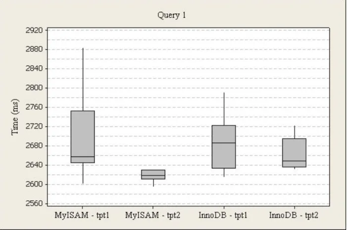
Figure 10. Power Test Query 1 Box Plot
The execution times for query one (net loss, manufacturer, and web page from the web returns cube), run one were higher for InnoDB (M=2961, SD=939) than MyISAM (M=2703, SD=90). For InnoDB, the times range from 2479ms to 5921ms, and 2633ms to 2722ms from the first to third quartile with a 2686ms median. For MyISAM, the times range from 2601ms to 2885ms, and 2644ms to 2753ms from the first to third quartile with a 2658ms median.
The execution times for query one, run two were higher for InnoDB (M=2929, SD=846) than MyISAM (M=2628, SD=35). For InnoDB, the times range from 2631ms to 5603ms, and 2636ms to 2695ms from the first to third quartile with a 2648ms median. For MyISAM, the
48
times range from 2549ms to 2706ms, and 2611ms to 2630ms from the first to third quartile with a 2618ms median.
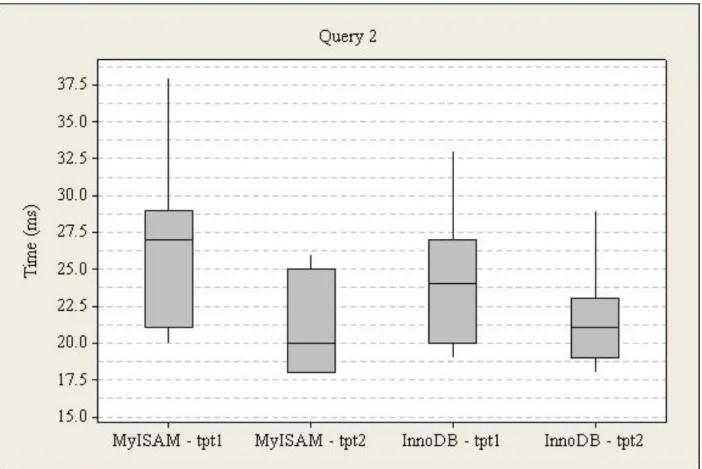
Figure 11. Power Test Query 2 Box Plot
The execution times for query two (store locations in Tennessee from the store sales cube with buying potential less than $500), run one were lower for InnoDB (M=25, SD=6) than MyISAM (M=25, SD=6). For InnoDB, the times range from 19ms to 41ms, and 20ms to 27ms from the first to third quartile with a 24ms median. For MyISAM, the times range from 20ms to 38ms, and 21ms to 29ms from the first to third quartile with a 27ms median.
The execution times for query two, run two were higher for InnoDB (M=21, SD=3) than MyISAM (M=20, SD=3). For InnoDB, the times range from 18ms to 29ms, and 19ms to 23ms from the first to third quartile with a 21ms median. For MyISAM, the times range from 18ms to 26ms, and 18ms to 25ms from the first to third quartile with a 20ms median.
49
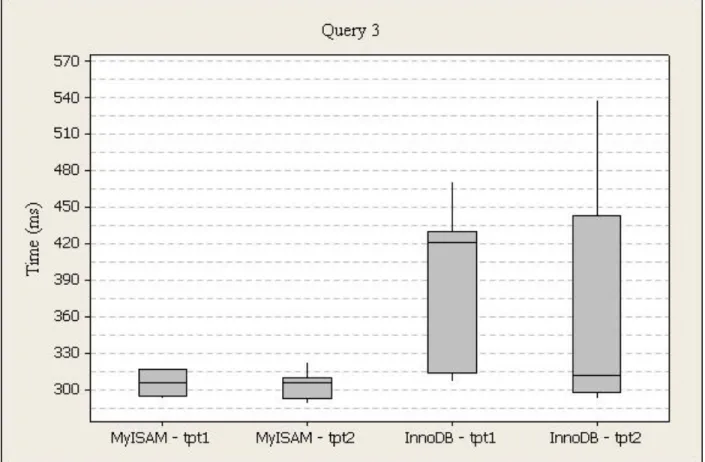
Figure 12. Power Test Query 3 Box Plot
The execution times for query three (profit for each item category, website member, and item category is music, home, or electronics from the web cube in 2000), run one were higher for InnoDB (M=389, SD=60) than MyISAM (M=330, SD=59). For InnoDB, the times range from 307ms to 472ms, and 314ms to 431ms from the first to third quartile with a 421ms median. For MyISAM, the times range from 293ms to 454ms, and 295ms to 317ms from the first to third quartile with a 306ms median.
The execution times for query three, run two were higher for InnoDB (M=353, SD=81) than MyISAM (M=302, SD=10). For InnoDB, the times range from 293ms to 539ms, and 298ms to 444ms from the first to third quartile with a 312ms median. For MyISAM, the times range from 289ms to 323ms, and 293ms to 310ms from the first to third quartile with a 306ms median.
50
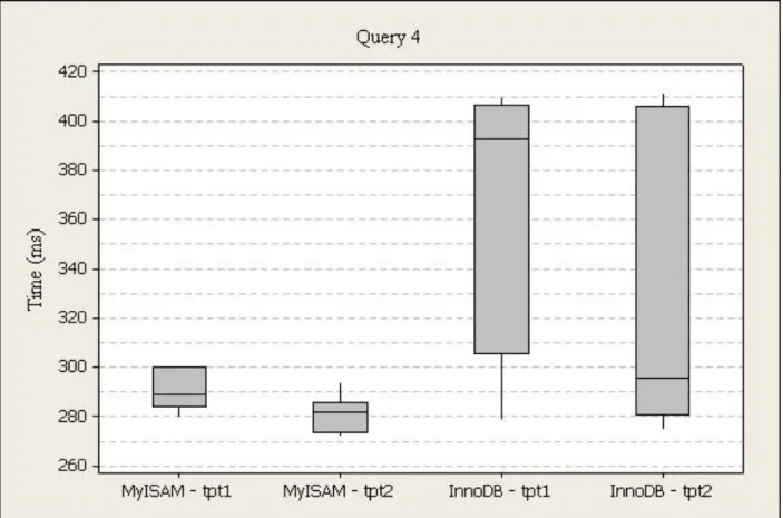
Figure 13. Power Test Query 4 Box Plot
The execution times for query four (profit for each item category, website member, and item category is in music, sports, or books from the web cube in 1999), run one were higher for InnoDB (M=362, SD=53) than MyISAM (M=313, SD=54). For InnoDB, the times range from 279ms to 410ms, and 306ms to 407ms from the first to third quartile with a 393ms median. For MyISAM, the times range from 280ms to 435ms, and 284ms to 300ms from the first to third quartile with a 289ms median.
The execution times for query four, run two were higher for InnoDB (M=345, SD=114) than MyISAM (M=281, SD=7). For InnoDB, the times range from 275ms to 674ms, and 281ms to 406ms from the first to third quartile with a 296ms median. For MyISAM, the times range from 272ms to 294ms, and 274ms to 286ms from the first to third quartile with a 282ms median.
51
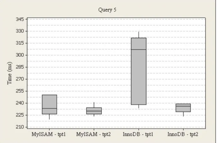
Figure 14. Power Test Query 5 Box Plot
The execution times for query five (total net loss from call centers managed by Larry McCray or Mark Hightower, and the item is in the home or books category from the catalog returns cube returned in 2002), run one were higher for InnoDB (M=288, SD=40) than MyISAM (M=251, SD=43). For InnoDB, the times range from 233ms to 330ms, and 238ms to 322ms from the first to third quartile with a 307ms median. For MyISAM, the times range from 219ms to 344ms, and 226ms to 250ms from the first to third quartile with a 233ms median.
The execution times for query five, run two were higher for InnoDB (M=276, SD=110) than MyISAM (M=230, SD=5). For InnoDB, the times range from 223ms to 614ms, and 229ms to 239ms from the first to third quartile with a 236ms median. For MyISAM, the times range from 223ms to 241ms, and 226ms to 234ms from the first to third quartile with a 230ms median.
52
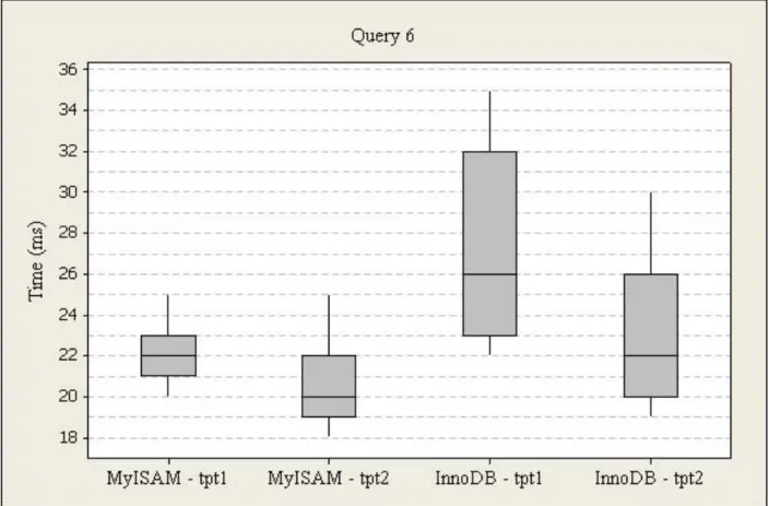
Figure 15. Power Test Query 6 Box Plot
The execution times for query six (quantity, item color, description, and info for four items from the inventory cube), run one were higher for InnoDB (M=27, SD=4) than MyISAM (M=22, SD=2). For InnoDB, the times range from 22ms to 35ms, and 23ms to 32ms from the first to third quartile with a 26ms median. For MyISAM, the times range from 21ms to 25ms, and 21ms to 23ms from the first to third quartile with a 22ms median.
The execution times for query six, run two were higher for InnoDB (M=23, SD=3) than MyISAM (M=20, SD=2). For InnoDB, the times range from 19ms to 30ms, and 20ms to 26ms from the first to third quartile with a 22ms median. For MyISAM, the times range from 18ms to 25ms, and 19ms to 22ms from the first to third quartile with a 20ms median.
53
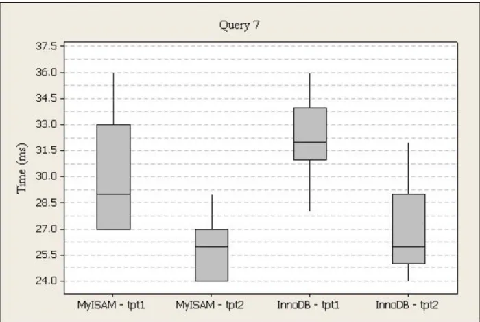
Figure 16. Power Test Query 7 Box Plot
The execution times for query seven (net loss, customer demographics, and date from the customer sales cube), run one were higher for InnoDB (M=32, SD=4) than MyISAM (M=30, SD=3). For InnoDB, the times range from 26ms to 41ms, and 31ms to 34ms from the first to third quartile with a 32ms median. For MyISAM, the times range from 27ms to 36ms, and 27ms to 33ms from the first to third quartile with a 29ms median.
The execution times for query seven, run two were lower for InnoDB (M=26, SD=3) than MyISAM (M=27, SD=6). For InnoDB, the times range from 24ms to 32ms, and 25ms to 29ms from the first to third quartile with a 26ms median. For MyISAM, the times range from 24ms to 47ms, and 24ms to 27ms from the first to third quartile with a 26ms median.
54
Figure 17. Power Test Query 8 Box Plot
The execution times for query eight (total quantity for the home and electronics categories from the catalog sales cube), run one were higher for InnoDB (M=24, SD=4) than MyISAM (M=21, SD=4). For InnoDB, the times range from 18ms to 32ms, and 23ms to 26ms from the first to third quartile with a 24ms median. For MyISAM, the times range from 18ms to 34ms, and 19ms to 21ms from the first to third quartile with a 20ms median.
The execution times for query eight, run two were higher for InnoDB (M=28, SD=29) than MyISAM (M=19, SD=3). For InnoDB, the times range from 17ms to 25ms, and 18ms to 24ms from the first to third quartile with a 19ms median. For MyISAM, the times range from 18ms to 26ms, and 18ms to 21ms from the first to third quartile with a 18ms median.