Optimal Spacecraft Formation Reconfiguration with Collision Avoidance
Using Particle Swarm Optimization
Haibin Huang
1, Yufei Zhuang
1, Guangfu Ma
2, Yueyong Lv
2 1Harbin Institute of Technology at Weihai, Weihai 264209, People’s Republic of China
2
Harbin Institute of Technology, Harbin 150001, People’s Republic of China e-mail: [email protected]
http://dx.doi.org/10.5755/j01.itc.41.2.854
Abstract. This paper pr esents an energ y-optimal trajectory planning method fo r spacecraft fo rmation reconfiguration in deep space environment using continuous lo w-thrust propulsion system. First, we emplo y the Legendre pseudospectral method (LPM) to transform the optimal reconfiguration problem to a parameter optimization nonlinear programming (NLP) problem. Then, to avoid the computational complexity for calculating the gradient information caused by traditional optimization methods, we use particle swarm optimization (PSO) algorithm to solve the NLP prob lem. Meanwhile, in order to avoid the collision between any pair of Legendre-Gauss-Lobatto (LGL) points, we insert some test points in the r egion where collision may happen most likely. What’s more, the collision avoidance constraints are also checked at these test points. Finally, numerical simulation shows that the energy-optimal trajectories for spacecraft reconfiguration could be generated by the method we proposed in a relative short time, so that it could be adopted on-board for practical spacecraft formation problems.
Keywords: formation reconfiguration; path planning; collision avoidance; Legendre pseudo spectral method; particle swarm optimization.
1. Introduction
The problem of s pacecraft formation has been extensively addressed recently because of the potential benefits of formation flying missions. One of these benefits lies in that the formation could be re-assigned to establish new science configurations that we need. The purpose of formation reconfiguration is to plan a set of optimal translational trajectories, along which each spacecraft of the formation is a ble to transfer from its current states to the desired final states, respectively, with a performance index (such as fuel, energy, time, etc.) in a given time interval [1]. Additionally, the problem of collision avoidance and control input limits should also be considered during the optimization.
The literature on formation reconfiguration can be categorized as deep space missions (the gravity free environment) and planetary orbital environment (POE) missions [2]. In deep space m issions, the spacecraft dynamics can be re duced to double integrator form, and varieties of fo rmation reconfiguration algorithms have been proposed in the literature. Richards et al. [3] proposed a Mixed Integer Linear Programming (MILP) method, which could find a g lobal optimized solution. However, the computation time wo uld increase dramatically with the increase of the number of spa cecraft or
computation steps. Additionally, it also needs to simplify the constraints formulation to a linear form, which makes the collision avoidance constraint conservative. Singh and Hadaegh [4] used polynomials of a variable order in time to parameterize the trajectories, but the algorithm is too complex. Cetin et al. [5] combined these two methods. The trajectories were first d iscretized in time u sing a cubic spline and then a feasib le MILP method was used to calc ulate the va riables at discretized points. These methods also take a lo ng time to solve the problem when t he number of computation steps increases and could not get a high accuracy neither. Many other approaches have also been used in formation reconfiguration, such as the RRT-based method [6] and the multiple-shooting method [7].
reconfiguration in near-earth orbit with an exact nonlinear relative spacecraft dynamic model.
Autonomous formation flying is important for deep space missions, so the reconfiguration algorithm for deep space missions should be simple enough to run on-board and plan the trajectories fast even real-time. However, the collision avoidance constraints usually result in a non-convex feasible solution space. The reconfiguration problem with collision avoidance constraints is NP-complete [1] which makes the problem hard to solve. These problems make the aforementioned methods suffer from an accelerated increase in computational complexity when the number of s pacecraft or the collocation points increases.
In this paper we presen t a novel method for trajectory planning of reconfiguration maneuvers of multi-spacecraft formation in deep space environment with continuous low-thrust control input. The basic problem discussed here is to find energy-optimal trajectories for the formation spacecraft in a relative short time. The s pacecraft is modeled as points of constant mass. Normally, the maneuver time is short and the propulsion systems used for maneuver are quite efficient, so the mass of each spacecraft is assumed to be c onstant during the whole reconfiguration.
2. Problem formulation
2.1. Statement of the problem
Consider the formation spacecraft in deep space earth-trailing formation flying, i.e. t hey are on an earth-trailing heliocentric orbit. When using linearized Hill equations to describe the motion of the formation spacecraft, it c an be shown that t he differential orbit force between two spacecraft is of the order of 1023
N. Because the reconfiguration usually oc curs in a relatively short time scale, ignoring the orbital forces between spacecraft in this work is well justified [10]. We assume that a to tal number of M spacecraft take
synchronous maneuvers in th e same time in terval [0, ]T . The system dynamics in deep space can be
stated as follows [11]: ( ) ( ) ( ), 1,2, , , [0, ]
l t l t l t
l M t T
X AX BU
(1)
where
3 3 3 3 3 3
3 3 3 3 3 3
[ , , , , , ] , [ , , ] , , 1
,
l l l
T T
l l l l l l l l x y z
l
x y z x y z u u u
m
X U
0 I 0
A B
0 0 I
( ) l t
X and Ul( )t are the state and c ontrol vectors of
the lth spacecraft at time t, respectively, mlis the mass
of the lth spacecraft.
The control inputs are assumed to be c ontinuous low-thrust forces confined to lie within specified limits
max l( )t max, 1,2, ,l M
U U U . (2)
The states at initial point and fi nal point are constrained with the following conditions
0
(0) ( )
l l
l T lT
X X
X X (3)
where Xl0 and XlT are the initial and final state vectors of the lth spacecraft.
Since the maneuvers time for all spacecra ft is the same, the objective function for the reconfiguration problem is to find Ul( )t , t[0, ]T , l1,2, , M, so that the energy consumption
1 0
1 ( )d
2 T M
T l l l
J t t
U U (4)is minimized.
2.2. Collision avoidance
It is obvious that, in order to avoid collisions, each spacecraft should be at least a specified distance away from others at any time step. Here each spacecraft is assumed to be a sph ere with a po int mass. Collision avoidance constraints can be stated as forbidden spheres associated with the spacecraft as follows [2]
2 2
safe
( ) ( ) , , 1,2, , ,
l t m t d
l m M l m
r r
(5)
where rl( )t is the radius vector of the lth spacecraft at time t, and dsafe is the minimum safety distance
between the centers of any two s pacecraft. These constraints change the problem into a no n-convex problem, which makes the formation reconfiguration problem difficult to solve.
3. Problem discretization using pseudospectral method
3.1. Legendre pseudospectral method
LetLN( )t denote the Legendre polynomial of order
N,and LN( )t be the first-order derivative of it. Letth, 0,1,2,
h N be the zeros of ( 2 1) ( )
N
t L t , with
0 1
t ,tN 1. These points are called LGL points,
which serve as collocation points of the system. Then we select the Nth order Lagrange interpolating
polynomials [12]
2
( 1) ( ) 1
( ) ,
( 1) ( ) 0,1,...,
N h
N h h
t L t
t
N N L t t t
h N
where h( )t satisfies the relationshiph( )tj hj. For a gi ven continuous function F t( )defined on [ 1,1] , the Nth degree interpolation polynomial is
0
( ) : N ( ) ( ) N
h h h
F t F t t
. (7)The integration of N( )
F t is
1
1 ( )d : 0 ( )
N N
h h h
F t t F t w
, (8)where
2
2 1
( 1) [ ( )] h
N h
w
N N L t
. (9)
The derivative of N( )
F t at the hth LGL point is
0
( ) N ( )
N
h hj j
j
F t D F t
(10)
where D: ( Dhj)is an (N 1) (N1) matrix, given by
( ) 1 ( )
( 1) 0
( ) : 4
( 1) 4
0 otherwise . N h
N j h j
hj
L t
h j
L t t t
N N
h j
D
N N
h j N
D (11)
3.2. Discretization for Reconfiguration Problem As LGL points lie in [ 1,1] , the optimal problem should be first restated by the linear transformation of the independent variable [13]:
2 0
0 0
t T
T T
. (12)
Then we extend LPM to multi-spacecraft case. The state and c ontrol vectors can be approximated using
h
, h0,1, , N
, 0 ( ) ( ) ( ), 1,2, , N N
l l l h h
h l M
X X X
(13) , 0 ( ) ( ) ( ), 1,2, , N N
l l l h h
h l M
U U U
(14) and , , 0 ( ) ,
1,2, , , 0,1, , . N
l h hj l j j
D
l M h N
X X
(15)
The integration term in J defined in the maneuvers
time interval [0, ]T can also be approximated as
, ,
0 d 0 ,
1,2, , . N
T T T
l l l h l h h h t w l M
U U U U
(16)
Thus, the trajectory planning problem can be translated into a nonlinear programming problem with undetermined parameters Xl h, and Ul h, , and minimizeing the objective function
, , 1 0 0 4 M N T l h l h h l h
T
J w
U U (17)subject to
, , ,
0
0 ( , , ) 0, 2
1,2, , , 0,1, , N
hj l j l h l h h j
T D
l M h N
X f X U
(18)
2 2
safe , , 0,
, 1,2, , , , 0,1, , l h m h
d
l m M l m h N
R R
(19)
,0 0
,
, 1,2, ,
l l
l T lT
l M X X
X X (20)
max max,
-Ul Ul Ul l1,2, , M (21) where Rl h, is the radius vector of the lth spacecraft at
the hth LGL point. The number of t he constraints
described by Equation (18) is 6 N M , and the
number of the constraints described by Equation (19) is 2
M
N C .
4. Optimization using Particle Swarm Optimization
4.1. Particle Swarm Optimization
Particle swarm optimization (PSO) is a stochastic optimization method which was invented by Kennedy and Eberhart in 1995 [14]. It is an ev olutionary algorithm that inspired by the social behavior of bird flocking or people grouping. In PSO, each possible solution is called a particle that is analogous to a bird in the bird flocking. The objective of the particles population (called swarm) is to find the global minimum of the fitness function (cost function). In each iteration, every particle updates by its own improving velocity which is derived from the personal best solution (known as ‘pbest’) and the global best position (known as ‘gbest’) discovered so far by the whole swarm. The basic PSO algorithm can be described as
1
, , 1 1 ( , , ) 2 2 ( , , )
k k k k k k k k
i h i h i h i h g h i h
where vi hk, and ,
k i h
x are the hth dimension velocity and
position of particle i in the kth iteration; pi hk, and pkg h,
are the hth dimension pbest and gbest of particle i in
the kth iteration; is a weighting factor known as
inertia; c1 is the cognitive weight and c2 is the social
weight; r1k and r2k are two random numbers in the
range of [0,1] . The new position of a particle is then calculated using
1 1
k k k
i i i
X X V . (23)
Here, k i
X and Vik are the position and velocity
vector of the ith particle during the kth iteration. We
use “ ” to dist inguish the position vector of PSO from the state vector of the reconfiguration problem.
When updating, a high velocity will dri ve the particles out of bounds or divergence, so the velocity of particle needs to be constrained. Set Vmax,has the maximum velocity of the hth dimension, then th e
formulation of velocity updating can be
1 1 , , 1 1 , , 1 max, max, , max, max, max, , , , . k k
i h i h
k k
i
h
h h
h i h
k i h
h h
v if v
v if v
if v V V V V V (24)
4.2. Optimization of Nonlinear Problem
In this se ction, we use PSO to solve the NLP discretized by LPM. When dealing with constraints, especially equality constraints, the PSO method needs to be modified. Several methods have been mentioned for this problem, such as eliminate the infeasi ble solutions method, penalty method, repair method, and so on. But for high dimensions constrained nonlinear optimization problems, it is alm ost impossible to find a feasible solution using these methods. Here, we make r1k and r2k the same for every dimension. Note
that the number of dimensions for one particle is ( 1) 9
M N , the ‘hth dimension’ mentioned below
contains M9 dimensions in fact, because it contains
M spacecraft and eac h of them has 3 position
variables, 3 velocity variables and 3 control input variables. We denote the hth dimension just for
convenience, i.e.:
0 0 0 0
, ,1 , ,1 , ,2 , ,2
0 0 , , , , 0 , , , , , , , [ ] 0,1,
i h i h i h i h i h M i h M i h
h N
X U X U
X U
X
(25)
Then using the method of linear particle swarm optimization (LPSO) [15], the following theorem is derived
Theorem 1: For each spacecraft, if all the position 0
i
X satisfy
0 0 0
, , , , , ,
0
0 ( , , ) 0, 2
0,1, , , 1,2, N
hj i j l i h l i h l h j
T D
h N l M
X f X U
(26)
and all the initial velocities 0
i
V satisfy
0
i 0
V (27)
then for any i teration k, Equation (18) is satisfied.
Here, both 0 , ,
i h l
X and Ui h l0, , are the variables to be
determined, they all belong to 0 ,
i h
X . We separate them
for convenience. Accordingly, 0 , ,
i h l
V and Vui h l0, , are the
initial velocities of 0 , ,
i h l
X and Ui h l0, , , and both of them
are the components of 0 ,
i h
V .
Proof: Since Pi0 is the local best of particle i and
0
g
P is the global best of all the particles, the following
equations can be derived
0 0 0
, , , , , ,
0
0,
2 2
0,1, , , 1,2, , N
hj i j l i h l ui h l j
T T
D
h N l M
P AP BP
(28)
0 0 0
, , , , , ,
0
0,
2 2
0,1, , , 1,2, , N
hj g j l g h l u g h l j
T T
D
h N l M
P AP BP
(29)
Using Equation (22) and Equation (27), we can derive
1 0 0 0 0 0 0
, , 1 1 , , , , 2 2 , , , ,
0,1, , , 1,2,
( ) ( ),
,
i h l i h l i h l g h l i h l
h N
c r c
l M r
V P X P X
(30)
1 0 0 0 0 0 0
, , 1 1 , , , , 2 2 , , , ,
0,1, , , 1,2, ,
( ) ( ),
ui h l c r ui h l i h l c r u g h l i h l
h N l M
V P U P U
(31)
Then, from Equations (28)-(31) we can derive
1 1 1
, , , , , ,
0
0,
2 2
0,1, , , , 1,2, , . N
hj i j l i h l ui h l j
T T
D
h N l M
V AV BV
(32)
From Equation (23), we can get
1 0 1
, , , , ,
0 0 0
1 1 ,
,
,
2 2
1,2, , .
N N N
hj i j l hj i j l hj i j l
j j j
i l i l
D D D
T T l M
AX BUX X V
(33)
Then we can derive
1 1
, , , , , ,
0 0 0
1 1
, ,
2 2
1,2, , .
N N N
h
k k k
i j
j hj hj
j j j
k k
i l i
l i
l
j l i j l
D D D
T T l M
AX BUX X V
That is
1 1 1
, , , , , ,
0
0 ( , , ) 0, 2
0,1, , , 1,2, , , 0. N
k k k
hj i j l i h l i h l h j
T D
h N l M k
X f X U
(35)
The above equations show that all the particles will fly through the hyperplane defined by the set of feasible solutions.
5. Solution approach
5.1. Initialization
We employ np particles to solve this problem, the initial positions of these np particles should satisfy Equation (26), and should guarantee that the formation spacecraft would not collide with eac h other. The operation steps are outlined as follows:
1. Optimize the reconfiguration problem without considering the collision avoidance, i.e., optimize the problem with the objective function (17) subject to Eq uation (18), (20) and (21). The solution of this optimization is defined as Ps. It will be use d when updating the velocity. Since the optimization of this problem is a simple convex optimization, this process could be worked out quickly.
2. For any two spacecraft l and m, find out the
point where the distance between them is nearest, noted as kl m, , kl m, [0,1, , ] N . 3. Initialize the npparticles using the objective
function
1
J (36)
subject to Equation (19), (21) and (22) with random initial solution guesses. So we could get a se rial of feasible solutions
0
i
X (i1,2, , np).
5.2. Iteration
Update the positions of al l the particles with Equation (23). The formulation to update the velocity is modified using
1
, , 1 1 , ,
2 2 , , 3 3 , ,
( )
( ) ( )
k k k k k
i h i h i h i h
k k k k k k
g h i h s h i h
v v c r p x
c r p x c r p x
(37)
where r3k is a ra ndom number in [0,1] , c3 is an acceleration coefficient. According to the experiments we can find that the best feasible trajectories of the reconfiguration problem always be found near the optimal trajectory obtain ed without collision avoidance constraints. So c r3 3k(pks d, xi dk, ) will drive
the particles towards the optimal trajectory, which
makes convergence faster than only using Equation (22). It can be proven as with Theorem 1 that Equation (18) is als o satisfied in any iteration with Equation (37). However, since Ps is not feasible, Equation (37) will drive the particles to infeasible region after some iterations. So we would eliminate c r3 3k(ps dk, xi dk, )
and use Equation (22) instead after 50 iterations. When using pseudospectral method or other collocation method, the cons traints are only satisfied at collocation points. So the sol ution may not be feasible between collocation points. More LGL points may solve this problem, but the computation time will also increase dramatically with the increas ing points. To ensure that the spacec raft would not collide with each other between the LGL points, we insert some time points, c alled test p oints between (kl m, 1) and
,
l m
k , and between kl m, and (kl m, 1) . The time at
these test points should be calculated using Equation (13) before iteration. And then, in eac h iteration, abandon the solutions which could not avoid the collision at these test po ints and t he LGL points. In this way, the final solution might be fea sible for the entire reconfiguration. Here, we choose the quadrisection points as the test points. Note that we can choose more or less tes t points according to the actual situation. It have little influence on the computation time.
If the values of the fitness functions of all the swarms do not improve in the last nstall generations or the generation maximum ng is reached, stop the optimization. The optimal state and c ontrol input vectors of every spacecraft will be the last global best position of the swarm.
6. Result
In this paper, we used the NLP solver, known as KNITRO, to generate every particle’s initial trajectories described by LPM. The software interfaced with Matlab, where the problem descriptions were performed. The problem was solved on a 2.1GHz personal computer with 2GB of RAM.
This example involves three spacecraft in three-dimensional space. It is assum ed that they take synchronous maneuvers in 10 time units. The initial and final positions are
1 1
2 2
3 3
(0) [0 0 0] , ( ) [15 15 15] , (0) [10 0 0] , ( ) [0 15 15] , (0) [10 0 10] , ( ) [0 15 0]
T T
T T
T T
T T T
r r
r r
r r
(38)
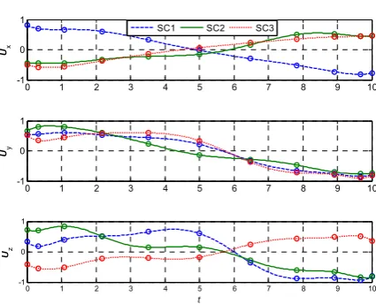
optimal trajectories of the three spacecraft are shown in Figure 1, where ‘SC’ means spacecraft. The distances between a ny two spacecra ft in the given time units are shown in Figure 2, where the mark ‘’ means the l ocations of the LGL points. The control inputs of the three spacecraft are shown in Figure 3, and the mark ‘’ also m eans the value of control inputs on each LGL point. The total energy consumption was 1 1.1958 units optimized by 145 generations. The history of the global best during iteration is shown in Figure 4.
Figure 1. Optimal trajectories of spacecraft
Figure 2. Distances between each pair of spacecraft
Figure 3. Control inputs of all spacecraft
Figure 4. Changes of the global best of all spacecraft
From Figure 4 we ca n find that the pr ocess converges fast at begi nning, and then evolves in a relative small region. After 50 iterations, all the particles converge to the global best value, which illustrates the good performance of our algorithm’s convergence. Figure 5 shows the energy consumption result from 200 Monte Carlo simulations with random initial values.
Figure 5. Evaluation through Monte Carlo simulations
From the results we can find that for a c ertain problem, this method could only find a near optimal solution, but not a certain optimal solution. However, this method could obtain a solution with collision avoidance in a short time which is shown in Table 1. Note that major time consumption is c aused by initialization, about 18 se conds, and t he iteration process only takes a very short time. The results also show that t here are no great changes i n the ene rgy index, which indicates that our algorithm is robust.
Figure 6 plots the re sults solved only by LPM using 10 LGL points with 9.9000 units of energy consumption. The NLP solver is also KNITRO. From this figure we can find that the dista nces between the spacecraft are almost zero between the 4th and 5th LGL points, though they would not collide with each other at t he LGL points. We also took 200 Monte
0 5
10 15
0 5 10 15 0
5 10 15
Y cordinate X cordinate
Z
co
rd
in
at
e
SC1 SC2 SC3
0 1 2 3 4 5 6 7 8 9 10
0 2 5 10 15 20 25
t
D
ist
an
ce
SC1-SC2 SC1-SC3 SC2-SC3
0 1 2 3 4 5 6 7 8 9 10
-1 0 1
Ux
SC1 SC2 SC3
0 1 2 3 4 5 6 7 8 9 10
-1 0 1
Uy
0 1 2 3 4 5 6 7 8 9 10
-1 0 1
t
Uz
0 25 50 75 100 125 150
11 12 13 14 15 16 17 18
Generation
E
ne
rg
y
In
dex
Mean Score Best Score Global Bests
0 20 40 60 80 100 120 140 160 180 200
10 11 12 13 14 15 16
No. of cases
E
ner
gy
In
de
Carlo simulations with random initial values f or the LPM. The comparison with PSO method is shown in Table 1. The nearest distance refers to the nearest distance between any two spacecraft. Note that the nearest distance and t he computation time are the average values for 200 Monte Carlo simulations. Maximum and minimum time are the maximum and minimum computation time of 200 Monte Carlo simulations. From the results we can find that, the PSO method could avoid most collisions during the whole maneuvers. Even if some collisions might occur between LGL points, the minimum distance between any two spacecraft was only a little sm aller than the safety distance. This situation could be acceptable because the safety distance is always conservative, moreover it al so happens occasionally. We can also see that the LPM could not avoid the collision with 10 LGL points, and the computation time vary a lot with different initial values. Even using 30 LGL points, the nearest distance between two spacecraft was still 1.5 units. The computation time increased to about 17 minutes.
Figure 6. Evaluation through Monte Carlo simulations with only LPM
Table 1. Contrast between the PSO method and the LPM
Method Distance Nearest Computation Time/s
Maximu
m Time/s m Time/s Minimu PSO 1.9138 19.9936 24.2913 16.7734 LPM 0.0862 17.8736 44.2292 5.5370
7. Conclusions
An efficient method for optimal reconfiguration of deep space spacecraft formation with collision avoidance is proposed in t his paper. Competitive computational efficiency is obtained by combining Legendre pseudospectral method and particle swarm optimization algorithm. Compared to typical collocation methods, more potential collisions occurring between spacecraft can be avoided by using this algorithm, which considers the collision
constraints between any pair of Legendre-Gauss-Lobatto points. Simulation results illustrate that t his method could solve the reconfiguration problem quickly so that it could be used on-board as a general approach for spacecraft form ation reconfiguration problems.
Acknowledgements
This work was supported in part by the N ational Science Foundation of China under the grant 61004072.
References
[1] A. B. Acikmese, D. P. Schar, E.A. Murray, F. Y. Hadaegh. A convex guidance algorithm for formation reconfiguration. AIAA Guidance, Navigation, and Control Conference and Exhibit, 2006.
[2] C. Sultan, S. Seereram, R. K. Mehra. Deep space formation flying spacecraft path planning. The International Journal of Robotics Research, Vol. 26, No. 4, 2007, 405-430. http://dx.doi.org/10.1177/02783
64907076709.
[3] A. Richards, T. Schouwenaars, J. P. How, E. Feron. Spacecraft trajectory planning with avoidance constraints using mixed-integer linear programming.
Journal of Guidance Control and Dynamics, Vol. 25, No. 4, 2002, 755-764. http://dx.doi.org/10.2514/2.49
43.
[4] G. Singh, F. Y. Hadaegh. Collision avoidance guidance for formation-flying applications. AIAA Guidance, Navigation, and Control Conference and Exhibit, 2001.
[5] B. Cetin, M. Bikdash, F. Y. Hadaegh. Hybrid mixed-logical linear programming algorithm for collision-free optimal path planning. IET Control Theory & Applications,Vol. 1, No. 2, 2007, 522-531.
[6] G. Aoude, J. How. Two-stage path planning approach for designing multiple spacecraft reconfiguration maneuvers. The 20th International Symposium on Space Flight Dynamics, 2007.
[7] M. Massari, F. B. Zazzera. Optimization of Low-thrust Reconfiguration Maneuvers for S pacecraft Flying in Formation. Journal of Guidance, Control, and Dynamics, Vol. 32, No. 5, 2009 , 1629-1638.
http://dx.doi.org/10.2514/1.37335.
[8] G. T. Huntington, A. V. Rao. Optimal reconfiguration of spacecraft formations using th e gauss pseudospectral method. Journal of Guidance, Control, and Dynamics, Vol. 31, No. 3, 2008, 689-698.
http://dx.doi.org/10.2514/1.31083.
[9] B. Wu, D. Wang, E. Poh, G. Xu. Nonlinear Optimization of Low-Thrust Trajectory for Satellite Formation: Legendre Pseudospectral Approach.
Journal of Guidance, Control, and Dynamics,Vol. 32, No. 4, 2009, 1371-1381. http://dx.doi.org/10.2514/
1.37675.
[10] Y. Kim, M. Mesbahi, F. Y. Hadaegh. Dual-spacecraft formation flying in deep s pace: optimal collision-free reconfigurations. Journal of Guidance, Control, and Dynamics, Vol. 26, No. 2, 2003, 375-379.
http://dx.doi.org/10.2514/2.5059.
0 1 2 3 4 5 6 7 8 9 10
0 2 5 10 15 20 25
t
D
ist
an
ce
7.2639 7.2639
10.4092 10.4093 10.4093
[11] D. P. Scharf, F. Y. Hadaegh, B. H. Kang. On the validity of the double integrator approximation in deep space formation flying. Proceedings of the international symposium Formation Flying Missions & Technologies, Toulouse, France, 2002.
[12] G. Elnagar, M. A. Kazemi, M. Razzaghi. The pseudospectral legendre method for discretizing optimal control problems. IEEE Transactions on Automatic Control, Vol. 40, No. 10, 1995, 1793-1796.
http://dx.doi.org/10.1109/9.467672.
[13] Q. Gong, F. Fahroo, I. M. Ross. Spectral algorithm for pseudospectral methods in optimal control. Journal of Guidance, Control, and Dynamics, Vol. 31, No. 3,
2008, 460-471. http://dx.doi.org/10.2514/1.32908.
[14] J. Kennedy, R. C. Eberhart. Particle swarm optimization. Proceedings of the IEEE International Conference on Neural Networks, Piscataway, NJ,
1995, 1942-1948.
http://dx.doi.org/10.1109/ICNN.1995.488968. [15] U. Paquet, A. P. Engelbrecht. A new particle swarm
optimizer for linearly constrained optimization.
Proceedings of the IEEE Congress on Evolutionary Computation, Piscataway, NJ, 2003, 227-233.