Learning to Predict One or More Ranks in
Ordinal Regression Tasks
Jaime Alonso, Juan Jos´e del Coz, Jorge D´ıez, Oscar Luaces, and Antonio Bahamonde
Artificial Intelligence Center. University of Oviedo at Gij´on, Asturias, Spain www.aic.uniovi.es
Abstract. We present nondeterministic hypotheses learned from an or-dinal regression task. They try to predict the true rank for an entry, but when the classification is uncertain the hypotheses predict a set of consecutive ranks (an interval). The aim is to keep the set of ranks as small as possible, while still containing the true rank. The justification for learning such a hypothesis is based on a real world problem arisen in breeding beef cattle. After defining a family of loss functions inspired in Information Retrieval, we derive an algorithm for minimizing them. The algorithm is based on posterior probabilities of ranks given an entry. A couple of implementations are compared: one based on a multiclassSVM and other based on Gaussian processes designed to minimize the linear loss in ordinal regression tasks.
1
Introduction
In the last few years, ordinal regression has become an important issue in Ma-chine Learning research. See [1] and [2] for a state of the art introduction. The aim of ordinal regression is to find hypotheses able to predict classes or ranks that belong to a finite ordered set. Applications include Information Retrieval [3], Natural Language Processing [4], collaborative filtering [5], finances [6], and user preferences [7].
The approach presented in this paper explores a new kind of predictions in ordinal regression. We shall build hypotheses that try to predict the true rank for an entry, but when the classification is uncertain the hypotheses predict an interval of ranks. The aim is to return a set of consecutive ranks, such that the set is as small as possible, while still containing the true rank. As we shall learn hypotheses for ordinal regression tasks with multiple outcomes, like nondeter-ministic automata, we shall call themnondeterministic ordinal regressors. From another point of view, these hypothesis could be called set-valued predictors.
Predictors of more than one class are not completely new. Given an error, the so called confidence machines, makeconformal predictions[8]: they produce a set of labels containing the true class with probability greater than 1−. Other approaches arose in the context of hierarchical organization of biological objects: predicting gene functions [9], or mapping biological entities into ontologies [10].
In the next Section we shall show the usefulness of these nondeterministic hypotheses in a real world application context: the assessment of muscle propor-tion in carcasses of beef cattle. This is an important quespropor-tion in cattle breeding since this proportion determines, on the one hand, the prices to be obtained by carcasses, and on the other hand, the genetic value of animals to select studs for the next generation.
We formalize the problem of nondeterministic predictions as a special kind of Information Retrieval. Thus, we define a family of loss functionsFβ and derive an algorithm for minimizing this loss. The algorithm needs the estimation of posterior probabilities of ranks given the entries. Then, we compare a couple of implementations built on the estimations provided by a SVM [11], and by the Gaussian approach of [1] devised for ordinal regression tasks.
The last Section of the paper presents an exhaustive set of experiments car-ried out in order to test the performance of the nondeterministic approach. Thus, in addition to the beef cattle learning task, we shall use 24 datasets publicly available that were previously used in ordinal regression tasks [1, 12].
2
The Round Profile of Bovines
The problem that motivated the research reported in this paper arose when we were trying to make reliable predictions of the value of the carcasses of beef cattle. This learning task was proposed by ASEAVA, the Association of Breeders of a beef breed of the North of Spain, Asturiana de los Valles. This is a specialized breed with many double-muscled individuals; their carcass have dressing percentages over 60%, with muscle content over 75%, and with a low (8%) percentage of fat [13]. The market target of these carcasses is made up of those consumers that prefer lean meat without any marbling [14, 7, 15]
Even if the animals are not going to be slaughtered, the prediction of car-cass value of a beef cattle is interesting since it can be considered as a kind of assessment that is useful for breeders to select the progenitors of the next generation. Thus, the ICAR (International Committee for Animal Recording) acknowledges as a good practice the recording of live animal assessments; since these assessments are a description of an animal’s morphology that reveals part of its economic value.
The records so obtained can be used for the evaluation of programs of genetic selection of dairy, dual purpose and specialized beef breeds. The growth of the scores over years of selection for specific goals can be seen as a measure of the success of the selection policy. On the other hand, when the assessed traits are heritable, the scores can be directly used for selection purposes given that they are capturing part of animal’s genetic value.
Traditionally, the assessment procedures were based onvisualappreciations of well trained technicians that had to rank a number of morphological char-acteristics that include linear lengths of significant parts of animals’ bodies. Although this process has been used successfully, it is clear that there is a prob-lem with the repeatability of the assessments; not only between assessors, but
!"#$%&&#&&'#()$*+$)"#$,*-(.$/,*01#$*+$%$2##+$3%41#$5&$%$'#%&-,#'#()$*+$)"#$
,*-(.(#&&$*+$)"#$15(#&$.,%6($5($)"#$/53)-,#&7$!"-&8$)"#$1#9'*&)$3*6$5&$%$
/%,%.5:'$*+$)"#$%(5'%1&$6"53"$"%;#$%$,%(<$*+$=8$6"51#$)"#$+*11*65(:$%,#$
,#/,#&#()%>;#$#?%'/1#&$*+$,%(<&$@8$A$%(.$B$,#&/#3>;#1C7
$$
Fig. 1.The assessment of the round profile of a beef cattle is a measurement of the roundness of the lines drawn in the pictures. Thus, the leftmost cow in the top row is a paradigm of the animals which have rank 1, while the following are representative examples of ranks 2, 3 and 4 respectively
even within assessors scoring the same animal in different times. In order to overcome these difficulties, we developed a new assessment method described in [16] that is almost completely repeatable and can be carried out using just 3 lengths (in centimeters) plus the appreciation of the curvature of the round profile (see the curves in Figure 1). For this learning task we used a kernel based method described in [17].
The aim of the assessment of round profiles is to rank the muscularity of animals. Therefore, it is a very important attribute for describing beef cattle. However, the curvature of the round profile is assessed by visualappreciations of experts. But visual appreciations is a source of problems. Thus, for instance, in [18], the authors describe an experiment in which a set of expert graders were asked to rank a collection of mushrooms into three major and eight subclasses of commercial quality. Grader consistency was assessed by repeated classification (four repetitions) of two 100-mushroom sets. Grader repeatability ranged from 6% to 15% misclassification.
Therefore, returning to beef cattle, to ensure the repeatability of the whole process, we should skip the subjective appreciation of the rank of round profiles. Thus, a new learning task arises: to estimate this rank from repeatable live animal descriptions. For this purpose, we built a dataset with 891 pairs of animal descriptions (6 lengths in centimeters of their bodies, live weight, and sex) and
ranks (in a scale of 1-4). To ensure a uniform criterion, the first author of this paper measured and ranked the round profile of the 891 live animals.
But this is a difficult learning task. The classification accuracy achieved by a multiclass SVM was 77%; the implementation used was a probabilisticlibsvm [11]. These results are not improved when using a learner specially devised for ordinal regression tasks. Thus, using the MAP approach of [1], the accuracy was 76%. The details about how we obtained these scores are included in the last section devoted to report a number of experimental results. On the other hand, we shall prove that a nondeterministic hypothesis contains the true class more than 84% of cases, while the average number of ranks predicted is just 1.21 or 1.30 depending of the learner used.
Moreover, the nondeterministic approach is more useful than the plain deter-ministic one in this problem for several reasons. First, the reliability of hypothesis predictions is higher than in the deterministic case. Therefore, when the hypoth-esis predicts only one rank, the estimation of the rank is very probably the true one. Second, when the prediction is an interval of more than one rank, we can appeal to a more expensive procedure to finally decide the true class. In this case, we may turn to an actualexpert, or we can wait until the natural growth of the animal make the classification more clear.
However, sometimes even a nondeterministic prediction may be useful to discard an animal as stud for the next generation: a prediction of [1,2] must imply a poor genetic value as meat producer, provided that the hypothesis is sufficiently reliable.
3
Formal Framework
LetX be an input space, andY a finite set of ordered ranks. Without any loss of generality, we can assume thatY ={1, . . . , k}for a givenk. We shall consider an ordinal regression task given by a training set S = {(x1, y1), . . . ,(xn, yn)}
drawn from an unknown distributionP r(X, Y) from the productX × Y. Within this context, we propose the following
Definition 1. A nondeterministic hypothesis is a function h from the input space to the set of non-empty intervals (subsets of consecutive ranks) of Y; in symbols,
h:X −→Intervals(Y). (1)
The aim of such a learning task is to find a nondeterministic hypothesish from a spaceHthat optimizes theexpected prediction performance (or risk)on samples S0 independently and identically distributed (i.i.d.) according to the distributionP r(X, Y):
R∆(h) =
Z
∆(h(x), y)d(P r(x, y)), (2)
where∆(h(x), y) is a loss function that measures the penalty due to the predic-tionh(x) when the true value isy.
In nondeterministic ordinal regression, we would like to favor those decisions of hthat contain the true ranks, and a smaller rather than a larger number of ranks. In other words, we interpret the output h(x) as an imprecise answer to a query about the right rank of an entry x ∈ X. Thus, the nondeterministic ordinal regression can be seen as a kind of Information Retrievaltask for each entry.
In Information Retrieval, performance is compared using different measures in order to consider different perspectives. The most frequently used are the Recall (proportion of all relevant documents that are found by a search) and Precision (proportion of retrieved documents that are relevant). The harmonic average of the two amounts is used to capture the goodness of a hypothesis in a single measure. In the weighted case, the measure is calledFβ. The idea is to measure a tradeoff betweenRecallandPrecision.
For further references, let us recall the formal definitions of these Information Retrieval measures. Thus, for a prediction of a nondeterministic hypothesish(x) with x ∈ X, and a rank y ∈ Y, we can compute the following contingency matrix, wherez∈ Y,
y=z y6=z
z∈h(x) a b
z /∈h(x) c d
(3)
where each entry (a, b, c, d) is the number of times that happens the correspond-ing combination of memberships. Thus, notice that a can only be 1 or 0, de-pending on whether the ranky is in the predictionh(x) or not;bis the number of ranks different from y included in h(x); c = 1−a; and d is the number of ranks different fromy that are not inh(x).
According to the matrix (Eq. 3), ifhis a nondeterministic hypothesis, and (x, y)∈ X × Y, we have the next definitions.
Definition 2. The Recallin aquery(i.e. an entryx) is defined as the propor-tion of relevant ranks (y) included inh(x):
R(h(x), y) = a
a+c =a= 1y∈h(x). (4) Definition 3. The Precision is defined as the proportion of retrieved ranks in h(x) that are relevant (y):
P(h(x), y) = a a+b =
1y∈h(x)
|h(x)| . (5)
In other words, given an hypothesis h, the Precision for an entry x, that is P(h(x), y), is the probability of finding the true rank (y) of the entry (x) by randomly choosing one of the ranks ofh(x).
Finally, the tradeoff is formalized by Definition 4. The Fβ, in general is defined by
Fβ(h(x), y) =
(1 +β2)a
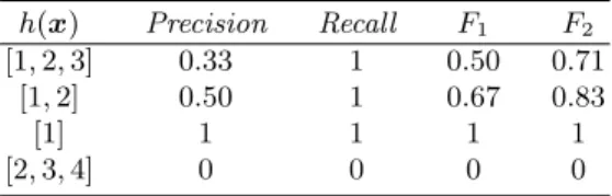
Table 1.For an entryxwith rank 1, (y= 1),Precision,Recall,F1, andF2for different
predictions of a nondeterministic classifierh
h(x) Precision Recall F1 F2
[1,2,3] 0.33 1 0.50 0.71
[1,2] 0.50 1 0.67 0.83
[1] 1 1 1 1
[2,3,4] 0 0 0 0
Thus, for a nondeterministic classifierhand a pair (x, y),
Fβ(h(x), y) =
( 1+β2
β2+|h(x)| if y∈h(x)
0 otherwise. (7)
The most frequently used F-measure isF1. For ease of reference, let us state
that
F1(h(x), y) =
2y∈h(x)
1 +|h(x)|. (8)
To illustrate the use of F-measures of an entry, let us consider an example. If we assume that the true rank of an entryxis 1, (y= 1), then, depending on the value ofh(x), Table 1 reports theRecall,Precision,F1, andF2. We observe
that the reward attached to a prediction containing the true rank with another extra rank ranges from 0.667 forF1to 0.833 forF2; while the amounts are lower
when the prediction includes 2 extra ranks.
Once we have the definition ofFβ for individual entries, it is straightforward to extend it to a test set. So, whenS0 is a test set of sizen, the average loss on it will be computed by R∆(h, S0) = 1 n n X j=1 ∆(h(x0j), yj0) = 1 n n X j=1 1−Fβ(h(x0j), y0j) (9) = 1 n n X j=1 1− 1 +β 2 β2+|h(x0 j)| 1y0 j∈h(x 0 j) ! .
It is important to realize that for a deterministic hypothesishthis amount is the average ”0/1” loss, since all predictions are singletons,|h(x)|= 1. Thus, the nondeterministic loss used here is a generalization of the error rate of deter-ministic classifiers. Furthermore, the average Recall and Precision on test sets can be similarly defined. In this case, theRecall on a test set is the proportion of times thath(x0) includesy0, and is thus a generalization of the deterministic accuracy.
Algorithm 1 The nondeterministic ordinal regressor nd •, an algorithm for computing the prediction with one or more ranks for an entryx provided that the posterior probabilities of ranks are given
Input:object descriptionx Input:{P r(j|x) :j= 1, .., k}
fori =1 to kdo
[Start+(i), P r Inter+(i)] = maxnPjt=+ji−1P r(t|x) :j= 1, . . . , k−i+ 1o /*P r Inter+(i) is the highest probability of the intervals of lengthi*/ /* This interval starts at classStart+(i) */
end for M in=argminn1−1+β2 β2+iP r Inter + (i) :i= 1, . . . ko returnˆ
Start+(M in), Start+(M in) +M in−1˜
4
How to Learn Intervals of Ranks with Posterior
Probabilities
In the general ordinal regression setting presented in Section 3, let x be an entry of the input spaceX, and let us now assume that we know the conditional probabilities of ranks given the entry,P r(rank=j|x) forj ∈ {1, . . . , k}. In this context, we wish to define
h(x) =Z∈Intervals{1, . . . , k} (10)
that minimizes the risk defined in (Eq. 2) when we use the nondeterministic loss given byFβ (Eqs. 6, 7, and 9). We shall prove that suchh(x) can be computed by Algorithm 1.
Proposition 1. (Correctness) If the conditional probabilitiesP r(j|x)are known, Algorithm 1 returns the nondeterministic predictionh(x)that minimizes the risk given by the loss1−Fβ.
Proof. To minimize the risk (Eq. 2), it suffices to compute ∆x(Z) = X y∈Y ∆(Z, y)P r(y|x) =X y∈Y (1−Fβ(Z, y))P r(y|x), (11)
withZ ∈Intervals{1, . . . , k}. Then, we only have to define
h(x) =argmin{∆x(Z) :Z∈Intervals{1, . . . , k}}. (12)
First we shall prove that when Z is an interval of lengthi, sayZ= [s, s+i−1], given x, the value of Equation (11) can be expressed in function of i and the probability of the interval. In fact, with a probability of 1−P r(Z|x), we expect a loss of 1: thetrue rank will not be one of the intervalZ. On the other hand, with the probability ofZ, the truerank will be in h(x), and therefore the loss
will be 1 minus the Fβ of the prediction h(x) =Z= [s, s+i−1]. In symbols, ∆x(Z) =∆x([s, s+i−1]) = 1− s+i−1 X j=s P r(j|x) 1 + s+i−1 X j=s P r(j|x) 1−1 +β 2 β2+i = 1−1 +β 2 β2+i s+i−1 X j=s P r(j|x). (13)
Therefore, the interval of lengthiwith lower loss starts atStart+(i) according
to the Algorithm 1; moreover, its loss is 1−1 +β
2
β2+iP r Inter
+(i). (14)
Thus if M in is the length that gives rise to the lowest loss, the output of the Algorithm is the value of Equation 12 as we wanted to prove.
In practice, posterior probabilities are not known: they are estimated by algo-rithms that frequently try to optimize the classification accuracy of a hypothesis that returns the class with the highest probability. In other words, probabilities are discriminant values instead of thorough descriptions of the distribution of classes in a learning task. Therefore, the actual role ofβin Algorithm 1 is that of a parameter that fixes the thresholds to decide the number of ranks to predict. Hence, like other parameters, β should be tuned in order to achieve optimal results. Thus, depending of the learning task and the probabilistic learner, to reach the highestF1scores, it might be necessary to use in Algorithm 1 a value
ofβ different from 1.
5
Experimental Results
In this section we report the results of a set of experiments designed to evaluate the nondeterministic learners proposed in this paper. The aim is to compare, on the one hand, the F1 scores of well known deterministic learners and their
nondeterministic counterparts. It may be argued that these comparisons are not completely fair since the F1 score tolerates predictions of more than one rank,
where it is easier to include the true one. In any case, we report these comparisons in order to test the capabilities of nondeterministic versions to achieve slightly better F1 scores than their deterministic counterparts. On the other hand, we
shall compare the Recall and size of predictions attained by nondeterministic learners.
Additionally, since we are dealing with ordinal regression tasks, we check the performance of nondeterministic algorithms in linear loss (sometimes called MAD, mean absolute deviation, orMAE, mean absolute error). For this purpose, we must assume singleton predictions; thus, we shall consider the center of each
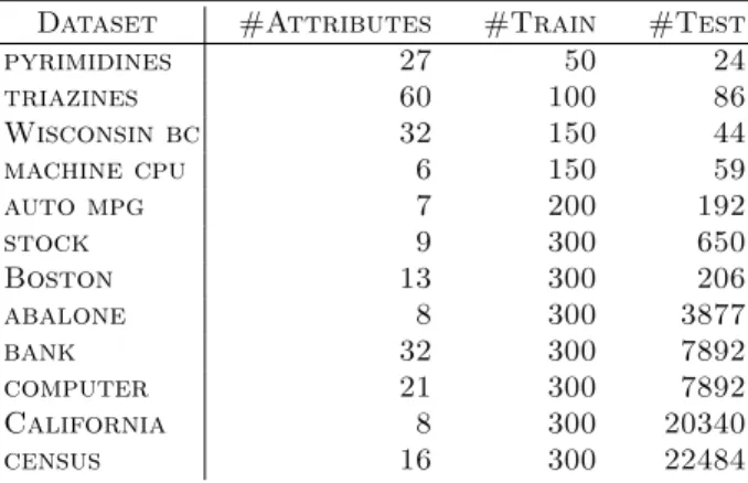
Table 2. Description of the datasets used in the experiments. The classes are real numbers, and they were discretized in 5 or 10 equal-frequency bins. The splits in train/test were suggested by the experiments reported in [1]
Dataset #Attributes #Train #Test
pyrimidines 27 50 24 triazines 60 100 86 Wisconsin bc 32 150 44 machine cpu 6 150 59 auto mpg 7 200 192 stock 9 300 650 Boston 13 300 206 abalone 8 300 3877 bank 32 300 7892 computer 21 300 7892 California 8 300 20340 census 16 300 22484
interval as the prediction attached to every intervalh(x). The idea is to consider that each rank r can be interpreted as the interval [r−0.5, r+ 0.5] in the real line; thus, a prediction of, say, [3,4] represents the real interval [2.5,4.5], and the center point is 3.5.
We used two kinds of learning tasks. In addition to the dataset of beef cattle profiles explained in Section 2, we used a collection of 12 benchmarks (Table 2) that were originally used for metric regression learning tasks. They are publicly available at Lu´ıs Torgo’s repository1. When they were used for ordinal regres-sion in papers like [1, 12], the continuous class values were discretized. We used versions with five and ten bins with the same frequency of training examples. The resulting rank values were ordered according to the original metric classes. To compare the performance of different approaches, we randomly split each data set into training/test partitions. Table 2 reports the characteristics of these datasets and the sizes of splits. The partition was repeated 20 times indepen-dently.
Since the nondeterministic approach proposed in this paper is based on the estimation of posterior probabilities of ranks, we used two alternative methods for this stage. First, we used a multiclassSVMthat estimates the probability of each class given an entry; the implementation used was libsvm [11]. The non-deterministic version built from it, following Algorithm 1, was called nd SVM. Second, we used theMAPapproach of [1] that was devised for ordinal regression tasks. It provides estimations of posterior probabilities using Gaussian processes. The nondeterministic counterpart was callednd MAP. The use of MAPin the experiments required reduced sizes of training sets (Table 2) similar to those
1
used in [1]. Nevertheless, the computational requirements of SVMwould allow us to usend SVM in tasks of bigger sizes.
Parameter setting. With theSVMwe used arbfkernel. To set the regularization parameterC and the rbf kernel parameterσ, we performed a grid search using a 2-fold cross validation repeated 5 times. The initial search was done with C ∈ {10−3, . . . ,103} (respectively σ ∈ {10−3, . . . ,102}) varying the exponent
in steps of 1. LetC0 andσ0 be the best parameters found; then followed a fine search fromC0−0.8 (respectively σ0−0.8) to C0+ 0.8 (respectivelyσ0+ 0.8) with a step of 0.2. Additionally, fornd SVMwe searched withinβ ∈ {0.5,1,1.5}, while the fine search explored the bestβ−0.2, and the bestβ+0.2. We looked for a β, instead of simply usingβ= 1, since we wished to compensate any possible inaccuracy in the estimation of probabilities.
TheMAP learner was used with its default parameters, and no additional tuning was required. The nondeterministic versionnd MAP used the search for β of thend SVM.
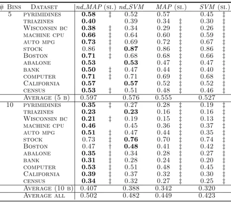
The scores achieved in F1 are shown in Table 3. The nondeterministic learner
based onMAPbears favorable comparison with the learner based onSVM. Thus, nd MAP wins in 18 out of 24 datasets, whilend SVM only wins 3 times out of 24; most of these victories are statistically significant using a Wilcoxon rank sum test of 1-tail over the 20 trials. Comparing the performance over the 24 datasets, we also appreciate significant differences (using a Wilcoxon test withp <0.01) in favor ofnd MAP. Therefore, the nondeterministic version ofMAPoutperforms the version based onSVMinF1when we are using sizes of training sets similar
to those showed in Table 2. In the comparison of deterministic versus nondeter-ministic, in all cases the nondeterministic version outperforms its deterministic counterpart; all but one cases are statistically significant withp <0.01.
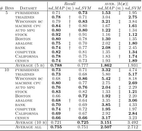
The scores inRecallare reported in Table 4. Again nd MAPwins in 17 out of 24 datasets, while nd SVM only wins 4 times out of 24; however, now the differences are not so frequently significant. To compareRecallscores with those achieved by the deterministic versions, let us remember that for deterministic algorithms, the proportion of successful predictions (accuracy) is also theF1and
theRecall. Therefore, comparing the last two columns of Table 3 and theRecall columns of Table 4, we appreciate that the nondeterministic learners outperform the deterministic versions. Thus, in 5 bins datasets, the differences are about 0.24, while in 10 bins datasets the differences are even higher: about 0.31. These results are logical since nondeterministic predictions have more opportunities to include the true ranks.
The average sizes of predictions are shown in the last two columns of Table 4. Here we observe that in the learning tasks of 5 bins these sizes in average are below 2, while with 10 bins, the predictions used more than 3 ranks in average. The explanation for these facts is straightforward. The nondeterministic al-gorithms tend to accumulate as many ranks as they are allowed by theF1; thus,
in tasks in which the deterministic learners have a poor performance, the corre-sponding nondeterministic learner may include more ranks in their predictions
Table 3. F1 scores of the two nondeterministic algorithms and their deterministic
counterparts. The results are the averages over 20 trials. In bold face we emphasize the highest score of each dataset. Additionally we test the statistical significance of some interesting differences: betweennd MAPandnd SVM(see the first column labeled by si.),nd MAPversusMAP(secondsi.column), andnd SVMversusSVM(lastsi. col-umn). The symbols†(respectively‡) show that differences are statisticallysignificant using a threshold of 0.05 (respectively 0.01) in a Wilcoxon rank sum test
# Bins Dataset nd MAP(si.)nd SVM MAP(si.) SVM (si.) 5 pyrimidines 0.58 ‡ 0.52 0.57 0.45 ‡ triazines 0.40 0.39 0.34 ‡ 0.30 ‡ Wisconsin bc 0.38 ‡ 0.34 0.29 ‡ 0.26 ‡ machine cpu 0.66 ‡ 0.64 0.60 ‡ 0.59 ‡ auto mpg 0.73 ‡ 0.69 0.72 ‡ 0.67 ‡ stock 0.86 † 0.87 0.86 ‡ 0.86 ‡ Boston 0.71 ‡ 0.68 0.68 ‡ 0.66 ‡ abalone 0.53 0.53 0.47 ‡ 0.47 ‡ bank 0.50 ‡ 0.47 0.44 ‡ 0.40 ‡ computer 0.71 ‡ 0.71 0.69 ‡ 0.68 ‡ California 0.57 0.57 0.52 ‡ 0.52 ‡ census 0.53 ‡ 0.51 0.48 ‡ 0.46 ‡ Average (5 b) 0.597 0.576 0.555 0.527 10 pyrimidines 0.35 ‡ 0.27 0.28 ‡ 0.19 ‡ triazines 0.23 0.23 0.16 ‡ 0.16 ‡ Wisconsin bc 0.21 ‡ 0.19 0.15 ‡ 0.13 ‡ machine cpu 0.46 0.45 0.36 ‡ 0.37 ‡ auto mpg 0.51 ‡ 0.47 0.44 ‡ 0.35 ‡ stock 0.73 ‡ 0.76 0.70 ‡ 0.74 ‡ Boston 0.47 † 0.48 0.41 ‡ 0.42 ‡ abalone 0.35 ‡ 0.34 0.28 ‡ 0.27 ‡ bank 0.31 ‡ 0.28 0.24 ‡ 0.20 ‡ computer 0.53 ‡ 0.51 0.48 ‡ 0.45 ‡ California 0.39 ‡ 0.37 0.32 ‡ 0.30 ‡ census 0.34 ‡ 0.32 0.27 ‡ 0.25 ‡ Average (10 b) 0.407 0.388 0.342 0.320 Average all 0.502 0.482 0.449 0.423
than in easier tasks. And it is clear that the learning tasks with 5 bins are easier than versions with 10 bins.
Considering the performance over all datasets, we can only find significant differences inRecallwithp <0.06; while the differences in size of predictions are definitively not significant.
Finally, Table 5 shows the scores achieved in linear loss. This is a relevant measure since we are dealing with ordinal regression learning tasks. Although the nondeterministic algorithms were not designed to improve the linear loss, we observe a good performance. Let us recall here that MAPis a state of the art learner for these tasks. In datasets of 5 bins, MAPwins nd MAP 8 times out of 12, with only 2 times out of 12 victories fornd MAP. Whilend MAPwins 7 times out of 12, against 4 wins out of 12 forMAP. The result is that differences over the 24 datasets are not statistically significant.
Table 4.Scores ofRecalland averagesizeof predictions (|h(x)|) for nondeterministic algorithms. Notice that for deterministic algorithms, the proportion of successful pre-dictions (accuracy) is also theF1and theRecall(see Table 3). The best scores for each
dataset are in bold. When the differences are statistically significant in a Wilcoxon rank sum test, they are marked with†(threshold of 0.05) or‡(0.01)
Recall aver.|h(x)|
# Bins Dataset nd MAP(si.)nd SVM nd MAP(si.)nd SVM 5 pyrimidines 0.71 0.73 1.53 ‡ 1.95 triazines 0.78 † 0.71 3.04 2.75 Wisconsin bc 0.79 † 0.83 3.21 ‡ 3.84 machine cpu 0.84 † 0.80 1.67 1.61 auto mpg 0.80 0.80 1.22 ‡ 1.34 stock 0.92 † 0.91 1.16 ‡ 1.12 Boston 0.80 0.78 1.30 1.35 abalone 0.75 ‡ 0.70 2.02 ‡ 1.80 bank 0.74 † 0.77 2.08 ‡ 2.45 computer 0.82 0.81 1.35 1.34 California 0.78 0.75 1.83 † 1.74 census 0.74 0.73 1.93 1.89 Average (5 b) 0.788 0.777 1.862 1.931 10 pyrimidines 0.73 0.71 3.32 ‡ 4.74 triazines 0.73 0.68 5.80 5.17 Wisconsin bc 0.68 ‡ 0.86 5.42 ‡ 8.18 machine cpu 0.80 0.77 2.75 2.69 auto mpg 0.76 0.76 2.04 ‡ 2.29 stock 0.83 0.82 1.33 ‡ 1.21 Boston 0.66 0.72 1.92 ‡ 2.20 abalone 0.68 † 0.64 3.35 ‡ 3.06 bank 0.70 0.69 3.85 ‡ 4.33 computer 0.74 † 0.72 1.95 1.97 California 0.69 0.67 2.92 2.84 census 0.66 0.66 3.17 3.23 Average (10 b) 0.721 0.725 3.151 3.492 Average all 0.755 0.751 2.507 2.712
On the other hand, in linear loss,nd MAPoutperformnd SVMin most of the datasets with differences statistically significant, see Table 5. The performance over all datasets is again statistically significant with p < 0.01. Finally, let us point out that the nondeterministic nd SVM outperforms (significantly with p <0.01)SVM.
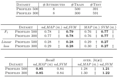
Profiles. Tables 6 summarize the scores achieved in the learning task described in Section 2. We used two datasets of sizes 300 and 500. The scores are quite similar for both sizes. Almost always,nd SVMoutperformsnd MAPsignificantly (p <0.01) in F1 and linear loss, although the scores are quite similar. On the
other hand, nd MAPis superior tond SVM in Recall, but again the scores are similar and the significance is only achieved withp <0.1 in one of the datasets. The differences are clearly significant (p <0.01) in the size of the predictions;
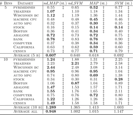
Table 5. Linear lossscores of the two nondeterministic algorithms and their deter-ministic counterparts. The lowest scores for each dataset are highlighted in bold. When the differences are statistically significant in a Wilcoxon rank sum test, they are marked with†(threshold of 0.05) or‡(0.01)
# Bins Dataset nd MAP(si.)nd SVM MAP(si.) SVM (si.) 5 pyrimidines 0.55 ‡ 0.65 0.52 † 0.77 ‡ triazines 1.07 1.10 1.18 ‡ 1.34 ‡ Wisconsin bc 1.12 ‡ 1.19 1.36 ‡ 1.44 ‡ machine cpu 0.48 0.48 0.45 ‡ 0.46 † auto mpg 0.32 ‡ 0.37 0.30 ‡ 0.35 ‡ stock 0.16 ‡ 0.15 0.14 ‡ 0.14 ‡ Boston 0.36 ‡ 0.41 0.34 ‡ 0.40 † abalone 0.72 † 0.73 0.72 0.75 ‡ bank 0.76 ‡ 0.83 0.76 0.90 ‡ computer 0.37 0.38 0.34 ‡ 0.36 ‡ California 0.63 † 0.62 0.59 ‡ 0.60 ‡ census 0.73 ‡ 0.77 0.71 ‡ 0.79 † Average (5 b) 0.607 0.640 0.618 0.692 10 pyrimidines 1.24 ‡ 1.88 1.31 † 2.25 ‡ triazines 2.23 2.21 2.79 ‡ 2.58 ‡ Wisconsin bc 2.44 2.48 3.08 ‡ 3.14 ‡ machine cpu 0.95 0.96 0.95 1.04 ‡ auto mpg 0.74 ‡ 0.80 0.69 ‡ 1.38 † stock 0.34 ‡ 0.30 0.31 ‡ 0.28 ‡ Boston 1.06 ‡ 0.87 1.04 ‡ 0.89 ‡ abalone 1.47 ‡ 1.53 1.57 ‡ 1.71 ‡ bank 1.55 ‡ 1.76 1.65 ‡ 2.11 ‡ computer 0.75 ‡ 0.76 0.72 ‡ 0.80 ‡ California 1.22 ‡ 1.26 1.26 ‡ 1.36 ‡ census 1.49 ‡ 1.58 1.58 ‡ 1.71 ‡ Average (10 b) 1.289 1.365 1.413 1.603 Average all 0.948 1.002 1.015 1.147
nd SVM only requires an average of 1.21 or 1.22 ranks to reach a proportion of 85% of predictions that contain the true rank.
6
Conclusions
We have presented a new kind of ordinal regressors: they are able to predict a variable number of consecutive ranks (an interval of ranks) for each entry. We call such set-valued hypotheses nondeterministic regressors. Roughly speaking, the approach presented in this paper addresses the problem of deciding what to predict when it is possible to envision that the label returned by a learning algorithm is uncertain. The utility of these predictions was illustrated in the context of a real world application: the assessment of muscle proportion in beef cattle carcasses.
After presenting the formal framework as a kind of Information Retrieval, we proposed a family of loss functions for nondeterministic ordinal regression: the complementary ofFβmeasures. Next we derived an algorithm to minimize such
Table 6. Profiles (see Section 2). Dataset characterizations, and scores achieved by deterministic and nondeterministic algorithms. All differences are statically significant (p <0.01) but those achieved inRecall(p <0.1)
Dataset #Attributes #Train #Test
Profiles 500 8 500 391
Profiles 300 8 300 591
Dataset nd MAP(si.)nd SVM MAP(si.)SVM(si.) F1 Profiles 500 0.78 ‡ 0.79 0.76 ‡ 0.77 ‡
Profiles 300 0.77 ‡ 0.78 0.76 ‡ 0.77 ‡
Linear Profiles 500 0.28 † 0.28 0.29 † 0.27 loss Profiles 300 0.29 ‡ 0.28 0.30 ‡ 0.27 ‡
Recall aver.|h(x)|
Dataset nd MAP(si)nd SVM nd MAP(si.)nd SVM Profiles 500 0.85 0.84 1.28 ‡ 1.21 Profiles 300 0.85 0.84 1.30 ‡ 1.22
loss functions provided we know the posterior probabilities of each rank given the entry to be ranked. To check the influence of the estimation of conditional probabilities we compared two implementations. The first one,nd SVMis based on a probabilisticSVM, while the second (nd MAP) is built onMAP, a learner specialized in ordinal regression learning tasks that uses Gaussian processes to estimate posterior probabilities.
The experiments reported in the previous Section show thatnd MAP out-performs nd SVM in almost all measures of performance. Therefore, it is clear the importance of having good probability estimations. However,MAPis slower thanSVM, and it is not possible to handle datasets of medium or large size with the approach based on Gaussian processes.
We think that the main goal of nondeterministic ordinal regressors is not to achieve similar (in fact better)Fβthan their deterministic counterpart. We would like to emphasize the dramatic improvement in the proportion of predictions that include the true rank, when the price to be paid for that increase is usually a tiny proportion of predictions with more than one rank.
Acknowledgements
The research reported here is supported in part under grant TIN2005-08288 from the MEC (Ministerio de Educaci´on y Ciencia of Spain). The authors acknowledge the help and partial support of the Association of Breeders ofAsturiana de los Valles, ASEAVA.
References
1. Chu, W., Ghahramani, Z.: Gaussian Processes for Ordinal Regression. The Journal of Machine Learning Research6(2005) 1019–1041
2. Cardoso, J., da Costa, J.: Learning to Classify Ordinal Data: The Data Replication Method. The Journal of Machine Learning Research8(2007) 1393–1429
3. Joachims, T.: Training linear SVMs in linear time. In: Proceedings of the ACM Conference on Knowledge Discovery and Data Mining (KDD), ACM (2006) 4. Shen, L., Joshi, A.: Ranking and Reranking with Perceptron. Machine Learning
60(1) (2005) 73–96
5. Yu, S., Yu, K., Tresp, V., Kriegel, H.: Collaborative ordinal regression. In: Pro-ceedings of the 23rd International Conference on Machine Learning (ICML’06). (2006) 1089–1096
6. Agarwal, A., Davis, J., Ward, T.: Supporting ordinal four-state classification deci-sions using neural networks. Information Technology and Management2(3) (2001) 5–26
7. del Coz, J.J., Bay´on, G.F., D´ıez, J., Luaces, O., Bahamonde, A., Sa˜nudo, C.: Trait selection for assessing beef meat quality using non-linear SVM. In Saul, L.K., Weiss, Y., Bottou, L., eds.: Advances in Neural Information Processing Systems 17 (NIPS ’04), Cambridge, MA, MIT Press (2005) 321–328
8. Shafer, G., Vovk, V.: A Tutorial on Conformal Prediction. Journal of Machine Learning Research9(2008) 371–421
9. Clare, A., King, R.: Predicting gene function in Saccharomyces cerevisiae. Bioin-formatics19(2) (2003) 42–49
10. Kriegel, H., Kroger, P., Pryakhin, A., Schubert, M.: Using Support Vector Machines for Classifying Large Sets of Multi-Represented Objects. Proc. 4thSIAM Int. Conf. on Data Mining (2004) 102–114
11. Wu, T.F., Lin, C.J., Weng, R.C.: Probability estimates for multi-class classification by pairwise coupling. The Journal of Machine Learning Research5(August 2004) 975–1005
12. Chu, W., Keerthi, S.S.: New approaches to support vector ordinal regression. In: Proceedings of the ICML’05, Bonn, Germany (2005) 145–152
13. Piedrafita, J., Quintanilla, R., Sa˜nudo, C., Olleta, J., Campo, M., Panea, B., Re-nand, G., Turin, F., Jabet, S., Osoro, K., Oliv´an, M.C., Noval, G., Garc´ıa, P., Garc´ıa, M., Cruz-Sagredo, R., Oliver, M., Gispert, M., Serra, X., Espejo, M., Garc´ıa, S., L´opez, M., Izquierdo, M.: Carcass quality of 10 beef cattle breeds of the Southwest of Europe in their typical production systems. Livestock Production Science82(1) (2003) 1–13
14. Luaces, O., Bay´on, G.F., Quevedo, J.R., D´ıez, J., del Coz, J.J., Bahamonde, A.: Analyzing sensory data using non-linear preference learning with feature subset selection. In Boulicaut, J.F., Esposito, F., Giannotti, F., Pedreschi, D., eds.: Pro-ceedings of the European Conference on Machine Learning and Principles and Practice of Knowledge Discovery in Databases (ECML/PKDD ’04), (2004) 286– 297
15. D´ıez, J., del Coz, J.J., Sa˜nudo, C., Albert´ı, P., Bahamonde, A.: A kernel based method for discovering market segments in beef meat. In: Proceedings of the 16th European Conference on Machine Learning - 9th European Conference on
Principles and Practice of Knowledge Discovery in Databases, ECML/PKDD’2005. Lecture Notes in Artificial Intelligence, Springer Verlag (2005) 462–469
16. Alonso, J., Bahamonde, A., Villa, A., Casta˜n´on, ´A.R.: Morphological assessment of beef catle according to carcass value. Livestock Science107(2007) 265–273 17. Bahamonde, A., Bay´on, G.F., D´ıez, J., Quevedo, J.R., Luaces, O., del Coz, J.J.,
Alonso, J., Goyache, F.: Feature subset selection for learning preferences: A case study. In Greiner, R., Schuurmans, D., eds.: Proceedings of the International Conference on Machine Learning (ICML ’04), (2004) 49–56
18. Kusabs, N., Bollen, F., Trigg, L., Holmes, G., Inglis, S.: Objective measurement of mushroom quality. In: Proc New Zealand Institute of Agricultural Science and the New Zealand Society for Horticultural Science Annual Convention, (1998)