MiningZinc: a Declarative Framework
for Constraint-based Mining
Tias Gunsa, Anton Driesa, Siegfried Nijssena,b, Guido Tackc, Luc De Raedta aDepartment of Computer Science, KU Leuven {firstname.lastname}@cs.kuleuven.be
bLIACS, Universiteit Leiden [email protected]
cFaculty of IT, Monash University, Australia and National ICT Australia (NICTA)
Abstract
We introduce MiningZinc, a declarative framework for constraint-based data mining. MiningZinc consists of two key components: a language component and an execution mechanism.
First, the MiningZinc language allows for high-level and natural modeling of mining problems, so that MiningZinc models are similar to the mathematical definitions used in the literature. It is inspired by the Zinc family of languages and systems and supports user-defined constraints and functions.
Secondly, the MiningZinc execution mechanism specifies how to compute solutions for the models. It is solver independent and supports both standard constraint solvers and specialized data mining systems. The high-level problem specification is first translated into a normalized constraint language (FlatZinc). Rewrite rules are then used to add redundant constraints or solve subproblems using specialized data mining algorithms or generic constraint programming solvers. Given a model, different execution strategies are automatically ex-tracted that correspond to different sequences of algorithms to run. Optimized data mining algorithms, specialized processing routines and generic solvers can all be automatically combined.
Thus, the MiningZinc language allows one to model constraint-based itemset mining problems in a solver independent way, and its execution mechanism can automatically chain different algorithms and solvers. This leads to a unique combination of declarative modeling with high-performance solving.
Keywords: Constraint-based mining, Itemset Mining, Constraint Programming, Declarative modeling, Pattern Mining
2010 MSC: 70, 90
1. Introduction
The fields of data mining and constraint programming are amongst the most successful subfields of artificial intelligence. Significant progress in the past few years has resulted in important theoretical insights as well as the development
of effective algorithms, techniques, and systems that have enabled numerous applications in science, society, as well as industry. In recent years, there has been an increased interest in approaches that combine or integrate principles of these two fields [1]. This paper intends to contribute towards bridging this gap. It is motivated by the observation that the methodologies of constraint pro-gramming and data mining are quite different. Constraint propro-gramming has focused on a declarative modeling and solving approach of constraint satisfac-tion and optimisasatisfac-tion problems. Here, a problem is specified through a so-called model consisting of the variables of interest and the possible values they can take, the constraints that need to be satisfied, and possibly an optimization function. Solutions are then computed using a general purpose solver on the model. Thus the user specifies what the problem is and the constraint programming system determines how to solve the problem. This can be summarized by the slogan constraint programming = model + solver(s).
The declarative constraint programming approach contrasts with the typical procedural approach to data mining. The latter has focussed on handling large and complex datasets that arise in particular applications, often focussing on special-purpose algorithms to specific problems. This typically yields complex code that is not only hard to develop but also to reuse in other applications. Data mining has devoted less attention than constraint programming to the issue of general and generic solution strategies. Today, there is only little sup-port for formalizing a mining task and capturing a problem specification in a declarative way. Developing and implementing the algorithms is labor inten-sive with only limited re-use of software. The typical iterative nature of the knowledge-discovery cycle [2] further complicates this process, as the problem specification may change between iterations, which may in turn require changes to the algorithms.
The aim of this paper is to contribute to bridging the methodological gap between the fields of data mining and constraint programming by applying the model + solverapproach to data mining.
In constraint programming, high-level languages such as Zinc [3], Essence [4] and OPL [5] are used to model the problem while general purpose solversare used to compute the solutions. Motivated in particular by solver-independent modeling languages, we devise a modeling language for data mining problems that can be expressed as constraint satisfaction or optimisation problems. Fur-thermore, we contribute an accompanying framework that can infer efficient execution strategies involving both specialized mining systems, and generic con-straint solvers. This should contribute to making data mining approaches more flexible and declarative, as it becomes easy to change the model and to reuse existing algorithms and solvers.
As the field of data mining is diverse, we focus in this paper on one of the most popular tasks, namely, constraint-based pattern mining. Even for the restricted data type of sets and binary databases, many settings (supervised and unsupervised) and corresponding systems have been proposed in the literature; this makes itemset mining an ideal showcase for a declarative approach to data mining.
The key contribution of this paper is the introduction of a general-purpose, declarative mining framework called MiningZinc. The design criteria for Min-ingZinc are:
• to support the high-level and natural modeling of pattern mining tasks; that is, MiningZinc models should closely correspond to the definitions of data mining problems found in the literature;
• to support user-defined constraints and criteria such that common ele-ments and building blocks can be abstracted away, easing the formulation of existing problems and variations thereof;
• to be solver-independent, such that the best execution strategy can be selected for the problem and data at hand. Supported methods should in-clude bothgeneral purpose solvers,specialized efficient mining algorithms and combinations thereof;
• to build on and extend existing constraint programming and data min-ing techniques, capitalizmin-ing on and extendmin-ing the state-of-the-art in these fields.
In data mining, to date there is no other framework that supports these four de-sign criteria. Especially the combination of user-defined constraints and solver-independence is uncommon (we defer a detailed discussion of related work to Section 6). In the constraint programming community, however, the design of the Zinc [3, 6] family of languages and frameworks is in line with the above cri-teria. The main question that we answer in this paper is hence how to extend this framework to support constraint-based pattern mining.
We contribute:
1. a novel library of functions and constraints in the MiniZinc language, to support modeling itemset mining tasks in terms of set operations and constraints;
2. the ability to define the capabilities of generic solvers and specialized al-gorithms in terms of constraints, where the latter can solve a predefined combination of constraints over input and output variables;
3. a rewrite mechanism that can be used to add redundant constraints and determine the applicability of the defined algorithms and solvers;
4. and automatic composition of execution strategies involving multiple such specialized or generic solving methods.
The language used is MiniZinc [7] version 2.0, extended with a library of functions and constraints tailored for pattern mining. The execution mecha-nism, however, is much more elaborate than that of standard MiniZinc. For a specific constraint solver, it will translate each constraint individually to a constraint supported by said solver. Our method can automatically compose execution strategies with multiple solvers.
The MiningZinc framework builds on our earlier CP4IM framework [8], which showed the feasibility of constraint programming for pattern mining. This work started from the modeling experience obtained with CP4IM, but the latter
contained none of the above contributions as it was tied to the Gecode solver and consisted of a low-level encoding of the constraints.
The present paper extends our earlier publication on MiningZinc [9] in many respects. It considers the modeling and solving of a wider range of data mining tasks including numeric and probabilistic data, multiple databases and pattern sets. The biggest change is in the execution mechanism, which is no longer restricted to using a single algorithm or generic solver. Instead, it uses rewrite rules to automatically construct execution plans consisting of multiple solver/al-gorithm components. We also perform a more elaborate evaluation, including a comparison of automatically composed execution strategies on a novel combi-nation of tasks.
Structure of the text. Section 2 introduces modeling in MiningZinc using the basic problem of frequent itemset mining. Section 3 illustrates how a wide range of constraint-based mining problems can be expressed in MiningZinc. In Section 4 the execution mechanism behind MiningZinc is explained, and Sec-tion 5 experimentally demonstrates the capabilities of the approach. SecSec-tion 6 describes related work and Section 7 concludes.
2. Modeling
MiningZinc builds on the MiniZinc modeling language and is hence suit-able for data mining problems that can be expressed as constraint satisfac-tion/enumeration or optimisation problems. We first introduce itemset mining and constraint-based mining. Using frequent itemset mining as an example, we demonstrate how this can be formulated as a constraint satisfaction problem in MiniZinc; and how this relates to the MiningZinc framework.
More advanced problem formulations and related tasks are given in the next section.
2.1. Pattern mining and itemset mining
Pattern mining is a subfield of data mining concerned with finding patterns, regularities, in data. Examples of patterns include products that people often buy together, words that appear frequently in abstracts of papers, recurring combinations of events in log files, common properties in a large number of observations, etcetera. Typical in pattern mining is that the pattern is a sub-structure appearing in the data, so not single words or events but collections thereof; and that there is a measure for the interestingness of a pattern, often based on how frequently it appears in the data.
We will focus on pattern mining problems where the patterns are expressible as sets, also called itemsets. Itemset mining was introduced by Agrawal et al. [10] as a technique to mine customer transaction databases for sets of items (products) that people often buy together. From these, unexpected associations between products can then be discovered.
Since its introduction, itemset mining has been extended in many directions, including more structured types of patterns such as sequences, trees and graphs.
A common issue with pattern mining techniques is that the number of patterns found can be overwhelming. In this respect, there has been much research on the use of constraints to avoid finding uninteresting patterns, on ways of removing redundancy among patterns, as well as different interestingness measures to be used. An overview can be found in a recent book [11].
The input to an itemset mining algorithm is an itemset database, containing a set oftransactionseach consisting of an identifier and a set ofitems. We denote the set of transaction identifiers as S = {1, . . . , n} and the set of all items as
I ={1, . . . , m}. An itemset databaseD maps transaction identifiers t ∈ S to sets of items: D(t)⊆ I.
Definition 1 (Frequent Itemset Mining). Given an itemset database D and a threshold Freq, the frequent itemset mining problem consists of finding all itemsetsI⊆ I such that|φD(I)| ≥Freq, where φD(I) ={t|I⊆ D(t)}.
The set φD(I) is called thecoverof the itemset. It contains all transaction identifiers for which the itemset is a subset of the respective transaction. The thresholdFreq is often called the minimum frequencythreshold. An itemsetI which has|φD(I)| ≥Freq is called afrequent itemset.
Example 1. Consider a transaction database from a hardware store:
t D(t) t D(t)
1 {Hammer, Nails, Saw} 4 {Nails, Screws, Wood}
2 {Hammer, Nails, Wood} 5 {File, Saw}
3 {File, Saw, Screws, Wood} 6 {Hammer, Nails, Pliers, Wood}
With a minimum frequency threshold of 3, the frequent patterns are: ∅,{Hammer},
{Nails}, {Hammer,Nails},{Wood},{Nails,Wood}.
Constraint-based pattern mining methods can leverage additional constraints during the pattern discovery process; cf. [10, 12, 13]. This has lead to the research topic of constraint-based itemset mining [14]. Section 3 will present different constraint-based mining problems in the context of MiningZinc. 2.2. Constraint Programming
Constraint Programming (CP) is a generic method for solving combinatorial constraint satisfaction (and optimisation) problems. It is a declarative method, in that it separates the specification of the problem from the actual search for a solution. On the language side, a number of declarative and convenient lan-guages have been developed. On the solver side, many generic constraint solvers are available, including industrial ones. We refer to the Handbook of Constraint Programming for an extensive overview of technologies and applications [15].
More formally, a Constraint Satisfaction Problem (CSP) is characterized by a declarative specification of constraints over variables.
Definition 2 (Constraint Satisfaction Problem (CSP)). A CSPP = (V,D,C) is specified by
• a finite set of variablesV;
• a domain D, mapping each variable V ∈ V to a set of possible values
D(V);
• a finite set of constraintsC.
A variableV ∈ Vis calledfixed if|D(V)|= 1. An assignment to the variablesV
is a domainDfor which all its variables are fixed. A domainD0is calledstronger than a domainDifD0(V)⊆ D(V) for allV ∈ V. AconstraintC(V
1, . . . , Vk)∈ C is an arbitrary Boolean function on variables {V1, . . . , Vk} ⊆ V. A solution to a CSP is an assignment to the variables such that all constraints are satisfied, where the domain D0 of the assignment must be stronger than D, e.g. in D0 each variableV can only be assigned to an element ofD(V).
Example 2. Imagine going on a boat trip. There is room to take 2 friends. Of 4 sailing friends, Sjarel and Kaat are better not put on a boat together; Kaat only wants to go if Nora goes; for Raf anything is fine. This can be modelled with a set variable F with domain {Sjarel,Kaat,Nora,Raf} and constraints
|F|= 2,{Sjarel,Kaat}*F,(Kaat ∈F)→(Nora∈F).
A range of practical modeling languages exist that aid a user in formulating a CSP. Example languages are MiniZinc [3], Essence [4] and OPL [5]. Such languages define variable types, such as Booleans, integers, sets and floats; and define a large number of constraints that can be specified. They typically provide a number of modeling conveniences such as syntactic sugar for accessing an element of an array, for looping over sets (e.g. forall, exists) and for using mathematical-like operators such as sums and products.
2.3. MiniZinc and itemset mining in MiniZinc
We build on the MiniZinc [6] modeling language, version 2.0. A MiniZinc model describes a constraint problem as a sequence of expressions, which can include parameter declarations, declarations of decision variables, function and predicate declarations, and constraints. A model describes a parametric prob-lem class, and it is instantiated by providing values for all the parameters, typ-ically in a separate data file. An important feature of MiniZinc is that models are solver-independent. They can be translated in a non-parameterized (in-stantiated) low-level format called FlatZinc that can contain solver-dependent constructs. This format is understood by a wide range of different types of solvers [16], such as CP solvers, MIP (Mixed Integer Linear Programming) solvers, SAT (Boolean Satisfiability) and SMT (SAT-Modulo-Theories) solvers. The solver reads and interprets the FlatZinc and computes solutions. The compiler achieves the specialization for a particular solver through the use of a solver-specificlibrary of predicate declarations. Such a library declares each basic constraint as either a solver builtin, which is understood natively by the target solver, or as a decomposition into simpler constraints that are supported by the solver.
Listing 1: “A simple MiniZinc model” 1 i n t: n ; 2 a r r a y[ 1 . . n ] o f v a r 1 . . n : q u e e n s ; 3 c o n s t r a i n t a l l d i f f e r e n t ( q u e e n s ) 4 /\ a l l d i f f e r e n t ( [ q u e e n s [ i ]−i | i i n 1 . . n ] ) 5 /\ a l l d i f f e r e n t ( [ q u e e n s [ i ]+ i | i i n 1 . . n ] ) ; 6 s o l v e s a t i s f y; 7 o u t p u t [show( q u e e n s ) ] ;
Listing 2: “Constraint-based mining”
1 i n t: N r I ; i n t: NrT ; i n t: F r e q ; 2 a r r a y[ 1 . . NrT ] o f s e t o f 1 . . N r I : TDB ; 3 v a r s e t o f 1 . . N r I : I t e m s ; 4 c o n s t r a i n t c a r d ( c o v e r ( I t e m s , TDB) ) >= F r e q ; 5 s o l v e s a t i s f y; 6 o u t p u t [show( I t e m s ) ] ;
Listing 1 shows a MiniZinc model of the n-Queens problem (the “Hello World”of constraint programming). The task is to placenqueens on ann×n chess board so that no two queens attack each other. Line 1 declares n as a parameter of the model. Line 2 declares an array of n decision variables, each corresponding to one row of the chessboard. Each decision variable has domain 1..n, which represents the column in which the queen in that row is placed (no two queens can be on the same row by definition). The require-ment to not attack is implerequire-mented by a conjunction (written/\) of three calls to the all different predicate, which constrain their arguments, arrays of expres-sions, to be pairwise different. The second and third constraints use array com-prehensions as a way of compactly constructing arrays corresponding to the di-agonals of the chess board, it is derived from the observation thatQi−Qj 6=i−j forbids left-to-right diagonals andQi−Qj 6= j−i forbids right-to-left diago-nals. Finally, the solve andoutputitems instruct the solver to find one solution (satisfy) and output the found values for the queens array. Note that a CP solver might declare that it supports the all different constraint natively in its library, whereas e.g. the library for a MIP solver would define a decomposition into linear inequalities.
Itemset mining in MiniZinc. Pattern mining problems can be modeled directly in MiniZinc. A MiniZinc model of the frequent itemset mining problem is shown in Listing 2. Lines 1 and 2 define the parameters and data that can be provided through a separate data file. The model represents the item and transaction identifiers inIandSby natural numbers from 1 toNrIand 1 toNrTrespectively.
Listing 3: “Constraint-based mining - cover” 1 f u n c t i o n v a r s e t o f i n t: c o v e r (v a r s e t o f i n t: I t e m s , 2 a r r a y[i n t] o f s e t o f i n t: D) 3 = l e t { v a r s e t o f i n d e x s e t (D ) : C o v e r ; 4 c o n s t r a i n t f o r a l l ( t i n ub ( C o v e r ) ) 5 ( t i n C o v e r <−> I t e m s s u b s e t D [ t ] ) 6 } i n C o v e r ;
The dataset D is implemented by the array TDB, mapping each transaction identifier to the corresponding set of items. The set of items we are looking for is modeled on line 3 as a set variable with an upper bound restricted to the set {1, . . . ,NrI}. The minimum frequency constraint is posted on line 4, which corresponds closely to the formal notation|φD(I)| ≥Freq.
The cover function on line 4 corresponds to φD(I). A distinguishing fea-ture of MiniZinc is its support for user defined-predicates, and since version 2.0, user-defined functions [7]. A MiniZinc predicate is a parametric constraint specification that can be instantiated with concrete variables and parameters, like in the call to all different in Listing 1. A MiniZinc function a generalisation to allow for arbitrary return values.
A declaration of thecoverfunction is shown in Listing 3. Recall that the for-mal definition of cover isφD(I) = {t|I ⊆ D(t)}. The implementation achieves this function by introducing an auxiliary set variable Cover (line 3) and con-straining it to contain exactly those transactions that are subsets ofItems. The
let { ... } in ... construct is used to introduce auxiliary variables and post con-straints, before returning a value, in this case the newly introducedCover, after the in keyword (line 6). Other MiniZinc functions used here include index set, which returns a set of all the indices of an array (similarly index set 1of2 returns the index set of the first dimension of a two-dimensional array), andub, which returns a valid upper bound for a variable. In this particular case, sinceCoveris a set variable,ub(Cover)returns a fixed set that is guaranteed to be a superset of any valid assignment to the Cover variable. Documentation on MiniZinc’s constructs is available online1.
In the cover () function of Listing 3, the introduced Cover variable is strained to be equal to the cover (in the let statement, lines 4–5). This con-straint states that for all valuestin the declared upper bound ofCover, i.e., all values that arepossibly inCover, the valuetis included inCoverif and only if it is an element of the cover, i.e. the setItemsis contained in transactiont. While the implementation of cover is not a verbatim translation of the mathematical definition, MiniZinc enables us to define this abstraction in a library and hide its implementation details from the users.
This example demonstrates the appeal of using a modeling language like
Listing 4: “Key abstractions provided by MiningZinc.” For brevity we write ‘set’ for ‘set of int’ and ‘array[]’ for ‘array[int]’.
1 f u n c t i o n v a r s e t: c o v e r (v a r s e t: I t e m s , 2 a r r a y[ ] o f s e t: TDB ) ; 3 f u n c t i o n v a r s e t: c o v e r (v a r s e t: I t e m s , 4 a r r a y[ , ] o f i n t: TDB ) ; 5 f u n c t i o n v a r s e t: c o v e r i n v (v a r s e t: C o v e r , 6 a r r a y[ ] o f s e t: TDB ) ; 7 f u n c t i o n v a r i n t: w e i g h t e d s u m (a r r a y[ ] o f v a r i n t: W e i g h t s , 8 v a r s e t: I t e m s ) ; 9 f u n c t i o n a r r a y[ ] o f s t r i n g: p r i n t i t e m s e t (v a r s e t: I t e m s ) ; 10 f u n c t i o n a r r a y[ ] o f s t r i n g: p r i n t i t e m s e t W c o v e r (v a r s e t: I t e m s , 11 a r r a y[ ] o f s e t: TDB ) ; 12 p r e d i c a t e m i n f r e q r e d u n d a n t (v a r s e t: I t e m s , 13 a r r a y[ ] o f s e t: TDB, 14 i n t: F r e q ) ; 15 f u n c t i o n ann: i t e m s e t s e a r c h (v a r s e t: I t e m s ) ; 16 p r e d i c a t e ann: e n u m e r a t e ; 17 f u n c t i o n ann: q u e r y (s t r i n g db , s t r i n g s q l ) ;
MiniZinc for pattern mining: the formulation is high-level, declarative and close to the mathematical notation, it allows for user-defined constraints like thecover relation between items and transactions, and it is independent of the actual solution method.
2.4. MiningZinc
In the example above we defined the cover function using the primitives present in MiniZinc. An important feature of MiniZinc is that common functions and predicates can be placed into libraries, to facilitate their reuse in different models. In this way, MiniZinc can be extended to different application domains without the need for developing a new language. The language component of the MiningZinc framework is such a library. Listing 4 lists the signatures of the key functions and predicates provided by the MiningZinc library; we discuss each one in turn.
The two key building blocks of the MiningZinc library are the cover and
cover inv functions. Given a dataset, the cover function determines for an item-set the transaction identifiers that cover it: φD(I) = {t|I ⊆ D(t)} and was already given in Listing 3.
The cover function is also defined over numeric data following the Boolean interpretation: a transaction is covered by an itemset if each item has a non-zero value in that transaction. Listing 5 shows the MiniZinc specification, which uses a helper function to determine the items in a transaction with non-zero value. This can be used together with other constraints on the actual numeric data, as we will show in the following section.
Listing 5: “cover constraint over numeric data” 1 f u n c t i o n v a r s e t o f i n t: c o v e r (v a r s e t o f i n t: I t e m s , 2 a r r a y[i n t ,i n t] o f i n t: DN) 3 = l e t { v a r s e t o f i n d e x s e t 1 o f 2 (DN ) : C o v e r ; 4 c o n s t r a i n t f o r a l l ( t i n ub ( C o v e r ) ) 5 ( t i n C o v e r <−> I t e m s s u b s e t row (DN, t ) ) 6 } i n C o v e r ; 7 f u n c t i o n s e t o f i n t: row (a r r a y[i n t ,i n t] o f i n t: DN, i n t: t ) 8 = {i | i i n i n d e x s e t 2 o f 2 (DN) w h e r e DN[ t , i ] != 0}
Listing 6: “cover inv function and the col helper function”
1 f u n c t i o n v a r s e t o f i n t: c o v e r i n v (v a r s e t o f i n t: C o v e r , 2 a r r a y[i n t] o f s e t o f i n t: D) 3 = l e t { v a r s e t o f min (D ) . . max (D ) : I t e m s , 4 c o n s t r a i n t f o r a l l( i i n ub ( I t e m s ) ) 5 ( i i n I t e m s <−> C o v e r s u b s e t c o l (D, i ) ) 6 } i n I t e m s ; 7 f u n c t i o n s e t o f i n t: c o l (a r r a y[i n t] o f s e t o f i n t: D, i n t: i ) 8 = {t | t i n i n d e x s e t (D) w h e r e i i n D [ t ]}
Listing 7: “Redundant minimum frequency constraint”
1 p r e d i c a t e m i n f r e q r e d u n d a n t (v a r s e t o f i n t: I t e m s , 2 a r r a y[i n t] o f s e t o f i n t: D, 3 i n t: F r e q ) 4 = l e t { v a r s e t o f i n t: C o v e r = c o v e r ( I t e m s , D) } i n 5 f o r a l l( i i n ub ( I t e m s ) ) ( 6 i i n I t e m s −> c a r d ( C o v e r i n t e r s e c t c o l (D, i ) ) >= F r e q 7 ) ;
The cover inv function computes for a set of transaction identifiers, the items that are common between all transactions identified. LetD0 be the transpose of D, that is, the database that maps items to sets of transaction identifiers.
D0(i) consists of the transactions in which itemiappears, that isD0(i) ={t∈
S|i∈ D(t)}. cover inv can now be defined similarly tocoveras follows: ψD(T) =
{i|T ⊆ D0(i)}. The MiningZinc specification is similar to that ofcoverand given in Listing 6; it includes a helper function to calculateD0(i).
The library includes other helper functions such asweighted sumand different ways to print item and transaction sets. The itemset search function defines a search annotation, which can be placed on the solve item to specify the heuris-tic that the solver should use. For MiningZinc, this function can be defined in solver-specific libraries, to enable the use of different search heuristics by different solvers.
con-straints that can be added automatically by the execution mechanism. A redun-dant constraint is already implied by the model – it does not express an actual restriction of the solution space – but it can potentially improve solver per-formance, e.g. by contributing additional constraint propagation. A predicate implementing a redundant constraint for minimum frequent itemset mining is shown in Listing 7. It uses the insight that if an itemset must be frequent, then each item must be frequent as well; hence, items that appear in too few transac-tions can be removed without searching over them. This can be encoded with a constraint that performslook-ahead on the items (Listing 7, line 6). See [8] for a more detailed study of this constraint. Another type of redundant information available in the library is a search annotation (Listing 4, line 15). This is an an-notation that can be added to the search keyword, and that specifies the order in which to search over the variables. An example of a search order that has been shown to work well for itemset mining isoccurrence[8]. We also added the enumeratesearch annotation to differentiate, in the model, between satisfaction (one solution) and enumeration (all solutions) problems. The last annotation is thequery keyword, which can be added to a variable declaration, for example
array [] of set : TDB :: query(”mydb.sql”, ”SELECT tid,item FROM purchases”);. The execution mechanism will automatically typecheck the expression, execute the query and add the data as an assignment to that variable. In this way, one can directly load data from a database, as is common in data mining.
A second instance of the above library exists, with the same signatures, but where all set variables are internally rewritten to arrays of Boolean variables, and all constraints and functions are expressed over these Boolean variables. This alternative formulation can sometimes improve solving performance, and it enables the use of CP solvers that do not support set constraints natively.
The MiningZinc library, without needing too many constructs, offers mod-eling convenience for specifying itemset mining problems; this will be demon-strated in the next section. Its elements will also be used by the framework described in Section 4 for detecting known mining tasks and when adding re-dundant constraints.
3. Example problems
Modeling a mining problem in MiningZinc follows the same methodology as modeling a constraint program: one has to express a problem in terms of variables with a domain, and constraints over these variables; for example, a set variable with a minimum frequency constraint over data.
From a data mining perspective, the kind of problem that can be expressed are enumeration or optimization problems that can be formulated using the variable types available in MiniZinc: Booleans, integers, sets and floats, and constraints over these variables. Many itemset mining problems fit this re-quirement (with the exception of greedy post-processing mechanisms such as Krimp [17] and other incomplete methods). We now illustrate how to model a range of diverse but representative itemset mining problems in MiningZinc.
Listing 8: “Constraint-based mining” 1 i n t: N r I ; i n t: NrT ; i n t: F r e q ; 2 a r r a y[ 1 . . NrT ] o f s e t o f 1 . . N r I : TDB ; 3 v a r s e t o f 1 . . N r I : I t e m s ; 4 c o n s t r a i n t c a r d ( c o v e r ( I t e m s , TDB) ) >= F r e q ; 5 % C l o s u r e 6 c o n s t r a i n t I t e m s = c o v e r i n v ( c o v e r ( I t e m s , TDB) ,TDB ) ; 7 % Minimum c o s t 8 a r r a y[ 1 . . N r I ] o f i n t: i t e m c ; i n t: C o s t ; 9 c o n s t r a i n t sum ( i i n I t e m s ) ( i t e m c [ i ] ) >= C o s t ; 10 s o l v e s a t i s f y : : e n u m e r a t e ;
3.1. Itemset Mining with constraints
Listing 8 contains some examples of constraint-based mining constraints that can be added to the frequent itemset mining model in Listing 2. Line 6,Items = cover inv(cover(Items,TDB),TDB), represents the popular closure con-straint I = ψD(φD(I)). This closure constraint, together with a minimum frequency constraint, represents theclosed itemset mining problem [18].
Lines 8/9 represent a common cost-based constraint [13]; it constrains the itemset to have a cost of at leastCost, withitem cost andCostbeing a user-supplied array of costs and a cost threshold.
We can use the full expressive power of MiniZinc to define other constraints. This includes constraints in propositional logic, for example expressing depen-dencies between (groups of) items/transactions, or inclusion/exclusion relations between elements. Two more settings involving external data are studied in the next section.
3.2. Itemset mining with additional numeric data
Additional data can be available from different sources, such as quantities of products (items) in purchases (transactions), measurements of elements (items) in physical experiments (transactions) or probabilistic knowledge about item/ transaction pairs. We look at two settings in more detail: high utility itemset mining and probabilistic itemset mining in uncertain data.
In high utility mining [19] the goal is to search for itemsets with a total utility above a certain threshold. Assumed given is an external utility e for each individual item, for example its price, and a utility matrixU that contains for each transaction alocal utility of each item in the transaction, for example the quantity of that item in that transaction. The total utility of an itemset is
P
t∈φD(I)
P
i∈Ie(i)U(t, i).Listing 9 shows the MiningZinc model corresponding to this task. Lines 3 and 4 declare the data, and lines 5 to 8 constrain the utility.
Listing 9: “High Utility itemset mining” 1 i n t: N r I ; i n t: NrT ; v a r s e t o f 1 . . N r I : I t e m s ; 2 % U t i l i t y d a t a 3 a r r a y [ 1 . . N r I ] o f i n t: I t e m P r i c e ; i n t: U t i l ; 4 a r r a y [ 1 . . NrT , 1 . . N r I ] o f i n t: UTDB ; 5 c o n s t r a i n t 6 sum ( t i n c o v e r ( I t e m s , UTDB) ) ( 7 sum ( i i n I t e m s ) ( 8 I t e m P r i c e [ i ]∗UTDB[ t , i ] ) ) >= U t i l ; 9 s o l v e s a t i s f y : : e n u m e r a t e ;
Listing 10: “Itemset mining with uncertain data”
1 i n t: N r I ; i n t: NrT ; v a r s e t o f 1 . . N r I : I t e m s ; 2 a r r a y [ 1 . . NrT , 1 . . N r I ] o f f l o a t: ProbTDB ; f l o a t: E x p e c t e d ; 3 c o n s t r a i n t 4 sum ( t i n c o v e r ( I t e m s , ProbTDB ) ) ( 5 p r o d u c t ( i i n I t e m s ) ( 6 ProbTDB [ t , i ] ) ) >= E x p e c t e d ; 7 s o l v e s a t i s f y : : e n u m e r a t e ;
It uses thecover function over numeric data (Listing 5, checks that a covered item is not 0), as well as the actual data to compute the utility.
Another setting is that of probabilistic itemset mining in uncertain data [20]. Listing 10 shows the MiningZinc model for this task. It is similar to the problem above, with the exception that the data is now real valued (including the numeric cover function), and the constraint (lines 3 to 6) is a sum-product. 3.3. Multiple databases
When dealing with multi-relational data, one can consider each relation as a separate transaction database. We distinguish two different cases: one where the relations are in a star schema, for example, items that are related to different transaction databases, and the more traditional multi-relational setting in which one can identifychains of relations.
When dealing with multiple transaction databases over the same set of items, one can impose constraints on each of the databases separately. For example, searching for the itemset with a minimum frequency ofαin one database and a maximum frequency ofβ in another.
A more advanced setting is that ofdiscriminative itemset mining. This is the task of, given two databases, finding the itemset whose appearance in the data is strongly correlated to one of the databases. Consider for example a transaction database with fraudulent transactions and non-fraudulent ones, and the task of finding itemsets correlating with fraudulent behavior. Many
Listing 11: “Discriminative itemset mining (accuracy)” 1 i n t: N r I ; 2 a r r a y[i n t] o f s e t o f 1 . . N r I : D f r a u d ; 3 a r r a y[i n t] o f s e t o f 1 . . N r I : D ok ; 4 v a r s e t o f 1 . . N r I : I t e m s ; 5 c o n s t r a i n t I t e m s = c o v e r i n v ( 6 c o v e r ( I t e m s , D f r a u d ) , D f r a u d ) ; 7 % O p t i m i z a t i o n f u n c t i o n 8 v a r i n t: S c o r e = c a r d ( c o v e r ( I t e m s , D f r a u d ) ) − 9 c a r d ( c o v e r ( I t e m s , D ok ) ) ; 10 s o l v e maximize S c o r e ;
different measures can be used to define what a good correlation is. This has led to tasks known as discriminative itemset mining, correlated itemset mining, subgroup discovery, contrast set mining, etc [21].
A discriminative itemset mining task is shown in Listing 11. This is an optimization problem, and the score to optimize is defined on line 8. One could also constrain the score instead of optimizing it; that is, add a threshold on the score and enumerate all patterns that score better. The score is p−n where pis the number of positive transactions covered and nthe number of negative ones. Optimizing this score (line 10) corresponds to optimizing the accuracy measure; see [22] for more details. An additional constraint ensures that the patterns are closed, but only on the transactions in the fraudulent transactions (one can show that there must always be a closed itemset that maximizes this score). Note how we reuse thecoverand cover inv functions that were also used in Listing 8.
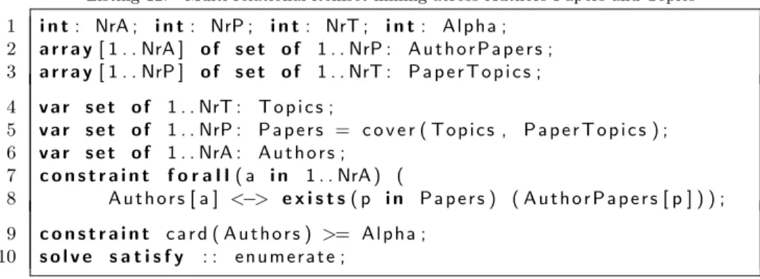
Multi-relational itemset mining consists of the extraction of patterns across multiple relations. Consider a database with authors writing papers on certain topics. A multi-relational mining task would be, for example, to mine for popular related topics, e.g. topics for which more thanαauthors have written a paper covering all topics. Listing 12 lists the MiningZinc model for this problem. Line 5 constrains the set of papers to those covering all topics, and line 8 states that authors must have at least one such paper.
Note how the existential relation on line 8 can be changed to variations of this setting, for example, requiring that authors have at least β such papers:
Authors[a] <−>sum(p in Papers) (AuthorPapers[p])>= Beta. Other (constraint-based) multi-relational mining tasks [23] can be expressed as well.
3.4. Mining pattern sets
Instead of mining for individual patterns, we can also formulate mining prob-lems over a setof patterns. For example, Listing 13 shows the specification of concept learningin ak-pattern set mining setting [24]. The goal is to find thek patterns that together best describe the fraudulent transactions, while covering
Listing 12: “Multi-relational itemset mining across Authors Papers and Topics” 1 i n t: NrA ; i n t: NrP ; i n t: NrT ; i n t: A l p h a ; 2 a r r a y[ 1 . . NrA ] o f s e t o f 1 . . NrP : A u t h o r P a p e r s ; 3 a r r a y[ 1 . . NrP ] o f s e t o f 1 . . NrT : P a p e r T o p i c s ; 4 v a r s e t o f 1 . . NrT : T o p i c s ; 5 v a r s e t o f 1 . . NrP : P a p e r s = c o v e r ( T o p i c s , P a p e r T o p i c s ) ; 6 v a r s e t o f 1 . . NrA : A u t h o r s ; 7 c o n s t r a i n t f o r a l l( a i n 1 . . NrA ) ( 8 A u t h o r s [ a ] <−> e x i s t s( p i n P a p e r s ) ( A u t h o r P a p e r s [ p ] ) ) ; 9 c o n s t r a i n t c a r d ( A u t h o r s ) >= A l p h a ; 10 s o l v e s a t i s f y : : e n u m e r a t e ;
few other transactions. It is very similar to the discriminative itemset mining setting, with the difference that it is assumed that multiple patterns are needed to find good descriptions of the fraudulent transactions.
Other problems studied in the context of k-pattern set mining and n-ary pattern mining [24, 25] can be formulated in a similar high-level way.
Pattern sets can have many symmetric solutions [24], which can slow down search. Symmetry breaking constraints can be added to overcome this, for exam-ple by lexicographically ordering the itemsets. MiniZinc offers predicates for lex-icographic constraints between arrays, but not between an array of sets. Using the helper function in Listing 14, one could add a symmetry breaking constraint to the concept learning problem of Listing 13 as follows: constraint lex less (Items );. 3.5. Combinations
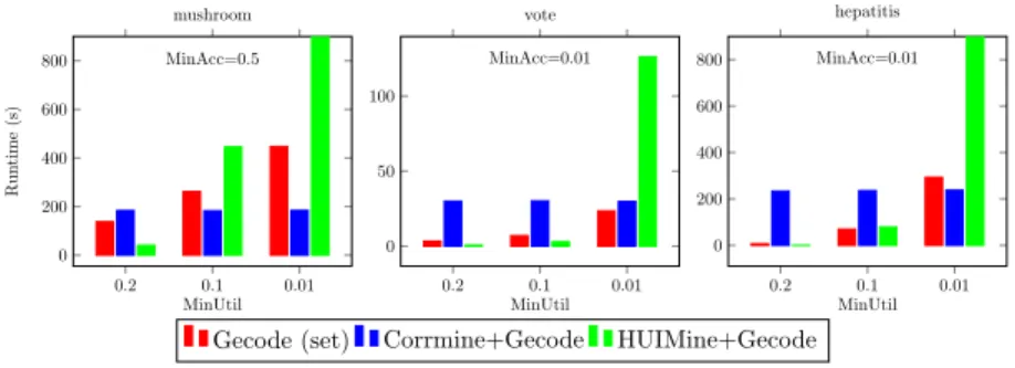
Using MiningZinc, we can also formulate more complex models. Listing 15 shows an example of such a model where we combine discriminative pattern mining (Listing 11) and high-utility mining (Listing 9).
We can use this model to find itemsets that both have a high utility and discriminate well between positive and negative transactions. To our knowledge, this combined problem has never been studied and no specialized algorithm exists. In Section 5 we show that several strategies exist to solve this model using MiningZinc.
4. MiningZinc execution mechanism
The MiniZinc language used in the previous section is declarative and solver-independent, as we did not impose what kind of algorithm or solving technique must be used. We now discuss how solving is done in MiningZinc.
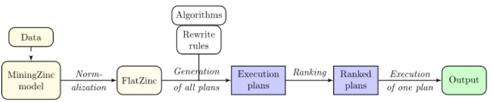
Figure 1 shows an overview of the overall execution mechanism. The starting point of the process is a MiningZinc model. When using a high-level language like MiniZinc, it is often possible to model a problem in various equivalent ways,
Listing 13: “Concept learning” 1 i n t: N r I ; i n t: K ; 2 a r r a y[i n t] o f s e t o f 1 . . N r I : D f r a u d ; 3 a r r a y[i n t] o f s e t o f 1 . . N r I : D ok ; 4 a r r a y [ 1 . . K ] o f v a r s e t o f 1 . . N r I : I t e m s ; 5 % c l o s e d on D f r a u d 6 c o n s t r a i n t f o r a l l( k i n 1 . . K) ( 7 I t e m s [ k ] = c o v e r i n v ( c o v e r ( I t e m s [ k ] , D f r a u d ) , D f r a u d ) ) ; 8 v a r i n t: S c o r e =% t o t a l f r a u d − t o t a l t o k 9 c a r d ( u n i o n( k i n 1 . . K) ( c o v e r ( I t e m s [ k ] , D f r a u d ) ) ) 10 − c a r d ( u n i o n( k i n 1 . . K) ( c o v e r ( I t e m s [ k ] , D ok ) ) ) ; 11 s o l v e maximize S c o r e ;
Listing 14: “Lex less for array of sets (lex less of two arrays is a MiniZinc global constraint)”
1 p r e d i c a t e l e x l e s s (a r r a y[i n t] o f v a r s e t o f i n t: S ) =
2 f o r a l l( k i n 1 . . l e n g t h ( S)−1) (
3 l e t { s e t: e l e m s = u n i o n( ub ( S [ k ] ) , ub ( S [ k + 1 ] ) ) } i n 4 l e x l e s s ( [ i i n S [ k ] | i i n e l e m s ) ] ,
5 [ i i n S [ k +1] | i i n e l e m s ] ) ) ;
Listing 15: “High Utility Discriminative itemset mining”
1 i n t: N r I ; i n t: NrPos ; i n t: NrNeg ; v a r s e t o f 1 . . N r I : I t e m s ; 2 % T r a n s a c t i o n d a t a 3 a r r a y[ 1 . . NrPos ] o f s e t o f 1 . . N r I : Pos ; 4 a r r a y[ 1 . . NrNeg ] o f s e t o f 1 . . N r I : Neg ; 5 % U t i l i t y d a t a f o r p o s i t i v e s 6 a r r a y [ 1 . . N r I ] o f i n t: I t e m P r i c e ; 7 i n t: M i n U t i l ; i n t: MinAcc ; 8 a r r a y [ 1 . . NrPos , 1 . . N r I ] o f i n t: UPos ; 9 c o n s t r a i n t 10 sum ( t i n c o v e r ( I t e m s , UTDB) ) ( 11 sum ( i i n I t e m s ) ( 12 I t e m P r i c e [ i ]∗UTDB[ t , i ] ) ) >= M i n U t i l ; 13 c o n s t r a i n t I t e m s = c o v e r i n v ( c o v e r ( I t e m s , Pos ) , Pos ) ; 14 c o n s t r a i n t c a r d ( c o v e r ( I t e m s , Pos ) ) − 15 c a r d ( c o v e r ( I t e m s , Neg ) ) >= MinAcc ; 16 s o l v e s a t i s f y : : e n u m e r a t e ;
MiningZinc model Data FlatZinc Norm-alization Execution plans Generation of all plans Algorithms Rewrite rules Ranked plans Ranking Output Execution of one plan
Figure 1: Overview of the MiningZinc toolchain
differing only in syntactic constructs used. The first step in the analysis pro-cess is hence to transform this model into a medium-level FlatZinc program (see Section 2.3), which we use as a normalized form for the analysis. This FlatZinc program is not suitable for solving, since it still uses the high-level MiningZinc predicates and functions. Given a set of algorithms and rewrite rules, the FlatZinc program is transformed into all possible sequences of algo-rithms that can solve the original problem; one such sequence of algoalgo-rithms is called an execution plan. Multiple execution plans are generated and ranked using a simple heuristic ranking scheme. When a plan is chosen (by the user, or by automatic selection of the highest ranked plan), each of the algorithms in that plan is executed to obtain the required output.
We now describe each of the components in turn. 4.1. Normalization
The purpose of converting to high-level FlatZinc is to enable reasoning over the set of constraints and to simplify the detection of equivalent or overlapping formulations.
FlatZinc is a flattened, normalized representation of a MiniZinc instance (a model and all its data). A MiniZinc instance is transformed into a FlatZinc pro-gram by operations such as loop unrolling, introduction of (auxiliary) variables in one global scope, simplifying constraints by removing constants, and rewrit-ing constraints in terms of simple built-ins, where possible. It also performs common subexpression elimination at the global scope: if two identical calls to an expression are present, one will be eliminated. For example, Listing 15 contains twice the functioncover(Items,Pos). In the FlatZinc code, only one call
X = cover(Items,Pos)will remain, and variableXwill be shared by all expressions that contained that call. More details of this procedure are described in [7].
Finally, FlatZinc also supports annotations, for exampleenumerate in List-ing 4. DurList-ing the flattenList-ing process, any annotation written in MiniZinc is passed to FlatZinc. Furthermore, any variable mentioned in theoutput state-ment receives aoutput var annotation. We will use the concept of output vari-ables versus non-output varivari-ables later.
For the purpose of normalization, we use a special version of the MiningZinc library that defines all MiningZinc predicates and functions as builtins, i.e. with-out giving a definition in terms of simpler expressions. The resulting FlatZinc is therefore not suitable for solving (no solver supports these builtins natively), but it can be analyzed much more easily than the original MiniZinc. It is also
much more compact than the FlatZinc generated for a CP solver, since in many cases the constraints do not need to be unrolled for every row in the dataset.
An important observation is that a FlatZinc program can be seen as a CSP (V,D,C), where the possible form of constraints inCis limited. More specifically, constraints are either of the form:
• p(X1, . . . Xn), where p ∈ P is a predicate symbol, and each Xi is ei-ther a variable in the CSP or a constant. Examples includeint le(Y,1), set subset(S,{2,4}); for notational convenience, in the examples we will represent some of these constraints in infix notation, i.e. Y ≤ 1, S ⊆ {2,4}.
• (X = f(X1, . . . Xn)), where f ∈ F is a function symbol and each Xi is either a variable in the CSP or a constant. Examples areY =set card(S) andT =cover(I, D), whereset card(S) is a function that calculates the cardinality of the set S, and cover(I, D) is as defined in Section 2. We refer to these constraints as functional definitions.
Consequently, in FlatZinc functions can only occur on the right-hand side of an equality constraint. Function and predicate symbols can be either built-in symbols or user-defined.
Example 3. Consider the problem of finding frequent itemsets on a given dataset, with minimum frequency of 20 and containing at least 3 items (Listing 2 + constraint card(Items) >= 3;). We will represent the datasets by{. . .}to indi-cate that it is a constant. After the automatic flattening process, the FlatZinc model obtained is the following (leaving the domain implicitly defined):
V={Items, T, SI, ST}
C={T =cover(Items,{...}), ST =card(T), SI =card(Items), ST ≥20, SI ≥3}
annotations={(Items,“output var”)}
This normalized model then needs to be transformed into an execution plan. 4.2. Generation of all plans
An execution plan specifies which parts of a MiningZinc model are handled by which algorithms or solving techniques. Concretely, an execution plan is a sequence of algorithms that together can handle all the constraints that are present in the model and hence produce the required output.
For example, a possible execution plan for the model of Example 3 could be to run theLCM algorithm [26] for frequent itemset mining to generate all itemsets of the given frequency, and then use a general purpose CP solver such as Gecode to filter the solutions further, only allowing itemsets with at least three elements.
This section will first describe the different algorithms that can be made part of MiningZinc, the rewrite rules to construct the plans and finally how all plans are generated using those rules.
4.2.1. Algorithms
We can distinguish two types of algorithms:
• specialized algorithms, which are only capable of solving specific combi-nations of constraints over input/output variables;
• CP systems, which are capable of solving arbitrary combinations of con-straints expressed in FlatZinc.
In an execution plan, the execution of an algorithm will be represented by an atom, consisting of a predicate applied to variables or constants.
Specialized algorithms. These are represented by predicates of fixed arity. Such predicates are declared through mode statements of the kind
p(±1V1, . . . ,±nVn),
wherepis the algorithm name,±i∈ {+,−}indicates themodeof a parameter andVi is a variable identifier for the parameter.
The interpretation of the modes is as follows:
• the input mode “+” indicates that the algorithm evaluating the predicate can only be run when this parameter is grounded, that is, its value is known;
• the output mode “-” indicates that the algorithm evaluating the predicate will only produce groundings for this parameter.
Example 4. The LCM algorithm for frequent itemset mining is character-ized by the mode statementLCM(+F,+D,−I), whereF represents a support threshold,D a dataset, andI an itemset. The predicate LCM(F, D, I) is true for any itemsetI that is frequent in dataset D under support thresholdF. A specific atom expressed using this predicate isLCM(10,{. . .}, Items).
In the MiningZinc framework, each specialised algorithm is registered with the following information:
• its predicate definitionp(±1V1, . . . ,±nVn);
• the set of FlatZinc constraints over V1, . . . , Vn that specify the problem this algorithm can solve (multiple sets can be given in case of multiple equivalent formulations);
• the binary executable of the algorithm;
• a way to map the input parameters of the predicate (in FlatZinc) to com-mand line arguments and input files for the algorithm;
• a way to map the output of the algorithm to output parameters (in FlatZinc).
Example 5. Version 5 of the LCM algorithm implements the frequent and closed itemset mining problems with additional support for a number of con-straints such as concon-straints on the size of an itemset and the size of the support (minimum and maximum). We can consider each combination of constraints as a different algorithm. For example, the instance of LCMv5 for closed itemset mining with an additional constraint on the minimum size of the itemset can be specified as follows:
predicate lcm5 closed minsize( +TDB, +MinFreq, +MinSize, -Items )
constraints: • C = cover(Items,TDB) • S = card(C) • int le(MinFreq, S) • iC = cover inv( C, TDB ) • set eq(Items,iC) • Sz = card(Items) • int le(MinSize, Sz) command
/path/to/lcm5 C -l MinSize infile(TDB) MinFreq outfile(Items) conversion infile,outfile: convert between FIMI format and FZN format In practice we provide syntax for describing multiple instances of the same algorithm in a more succinct way.
CP systems. In contrast to specialized algorithms, CP systems can operate on an arbitrary number of variables and constraints. A predicate representing a CP system can therefore take an arbitrary number of variables as parameter; furthermore, we assume that it is parameterized with a set of constraints.
Example 6. A predicateGecodeC(V1, . . . , Vn) represents the Gecode CP sys-tem, where V1, . . . Vn are all variables occurring in the constraint set C with which the system is parameterized. A specific atom expressed using this pred-icate isGecodeC(I, T, ST), whereC ={T =cover(I, D), ST =card(T), ST ≥ 20}; this predicate is true for all combinations of I, T and ST for which the given constraints are true.
A CP system is capable of finding groundings for all variables that are not grounded, and hence there are no mode restrictions on the parameters. Typi-cally, some of the variables occurring in the constraints are not yet grounded, requiring the CP system to search over them. In case all variables are already grounded when calling the CP system, the system only has to check whether the constraints are true.
In the MiningZinc framework, each CP system is registered with the follow-ing information:
• its predicate name (e.g. Gecode);
• the set of FlatZinc constraints it supports, includingglobal constraints;
• the binary executable of the CP system;
• optionally, whether set variables must be translated to a Boolean encoding before executing the CP system (more on this in Section 4.2.3).
Execution plans. With the two types of algorithm predicates introduced, we can now define an execution plan as a sequence of atoms over algorithm predicates. Sequences have to be mode conform, that is, an algorithm must have its input variables instantiated when it is called.
Example 7. For the model of Example 3 the following is a valid execution plan that uses the LCM and Gecode predicates of Example 4 and 6:
[LCM(10,{. . .}, I),Gecode(SI=card(I),SI≥3)(I)].
The main challenge is now how to transform the initial FlatZinc program into an execution plan. The rewrite rules used to do so are described in the next section.
4.2.2. Rewrite rules
We use rewriting to transform a FlatZinc program into an execution plan. Specifically, we describe astateof the rewrite process with a tuple
(L, C),
whereLis an execution plan, andC is a set of constraints and annotations. The initial state in the rewrite process is (∅, C), where C is the set of all FlatZinc constraints and the empty set indicates the initially empty execution plan; the final state in the rewrite process is (L,∅), whereL represents a valid execution plan for the initial set of constraintsC, and the empty set indicates that all constraints have been evaluated in the execution plan (modulo the optionalannotations). Rewrite rules will transform states into other states; an exhaustive search over all possible rewrites will produce all possible execution plans.
A key concept in these rewrite rules are substitutions. Formally, a substi-tutionθ ={V1/t1, . . .} is a function that maps variables to either variables or constants. IfC is an expression, byCθ we denote the expression in which all variablesVi have been replaced with their corresponding valuesti according to θ. If for substitution θ it holds thatCθ ⊆C0, the set of constraintsC is said toθ subsumethe set of constraints C0. In the exposition below predicates and variables are untyped for ease of presentation. FlatZinc is a typed language, so in practice we only allow variables of the same type to be mapped to each other. We now define three types of rewrite rules: rules for adding redundant con-straints, for executing specialized algorithms and for executing CP systems.
Rules for redundant constraints. LetC1andC2both be sets of constraints over the same variables, letC1→C2hold (C1entailsC2). SinceC2will be true wheneverC1is, the set of constraintsC2can be added as redundant constraints to anyC⊇C1. Taking substitutions into account, we have the following rewrite rule:
IF C1θsubsumes the set of constraintsC, THEN (L, C)`(L, C∪C2θ).
Example 8. Past work showed that the execution of the frequent itemset mining task is more efficient in some CP systems if a look-ahead constraint is added. Let C2 = {minfreq redundant(I, D, V)} represent this look-ahead constraint (see Section 2.4). This constraint set is entailed by the set of con-straintsC1={A=cover(I, D), B=card(A), V ≤B}. Then for the model of Example 3 (depicted byCM) we have the following rewrite:
(∅, CM)`(∅, CM ∪ {minfreq redundancy(I,{. . .},20)}).
Redundant constraints are registered in the system with the following infor-mation:
• a set of constraintsC1;
• a function that takes as input the substitutionθand produces a constraint setC2 over the variables inθas output.
Rules for specialized algorithms. Recall that all specialised algorithms are registered with a predicate definitionp(±1V1, . . . ,±nVn) and a set of constraints C that define the problem being solved by this algorithm. Note that not all variables inC need to be a parameter of the predicate; there can beauxiliary variables.
Let (L, CM) be a state in the rewriting of an execution plan. The key idea is that if the set of constraints C of an algorithm subsumes the given set of constraintsCM, then we wish to append its predicate (p) to the execution plan L. More formally, ifLis the current plan, andCsubsumesCMwith substitution θ, we can addp(V1θ, . . . , Vnθ) toL.
Example 9. If our model has constraints{T =cover(I,{. . .}), ST =card(T), SI= card(I), ST ≥20, SI≥3}, and our current execution plan is empty (∅); LCM’s constraint set {T0 = cover(I0, D0), ST0 = card(T0), ST0 ≥ V0} subsumes the model with the substitution{T0 7→T, I07→I, D07→ {. . .}, V0 7→20}. Hence, we may addLCM(20,{. . .}, I) to the execution plan.
Removing subsumed constraints from CM. The next important step is to re-move as many subsumed constraints as possible fromCM, to avoid them being unnecessarily recomputed or verified again. Indeed, running the algorithm will ensure that these constraints are satisfied, but unfortunately, we cannot always remove all subsumed constraints.
Example 10. If our model has constraints{T =cover(I,{. . .}), ST =card(T), ST ≥20, ST ≤40}, and we again use the LCM algorithm to solve part of this model, we cannot remove the constraints ST =card(T) and T =cover(I, D), even though they are subsumed; the reason is that the constraint ST ≤ 40, which is not subsumed, requires theST value, which is not in the output of the LCM algorithm.
This problem is caused by auxiliary variables, which occur in the constraint definition of the algorithm but not in the mode definition.
WhenCθis the set of constraints subsumed by the algorithm, the setCM\Cθ contains all remaining constraints; if among these remaining constraints there are constraints that rely on the functionally defined by variables that are not in the mode definition of the algorithm, we can remove all constraints except the functional definition constraints necessary to calculate these variables.
More precisely, assume we are given a state (L0, C0) for a FlatZinc program with constraints C and output variables Voutput (that is, variables in V that
have aoutput var annotation). Then let V(L0,C0) be the set of those variables
occurring in C0 or in Voutput that do not occur in L0, e.g. the free variables
that will still be used later in the execution plan. LetF(L0, C0,C) = (L0, C0∪ {c ∈ C |c functionally defines a variable inV(L0,C0)}), i.e., this function adds
the functional definitions for variables for which the definitions are missing from C0. The inclusion of missing definitions may trigger a need to include further definitions; the repeated application of this function will yield a fixed point F∗(L0, C0,C).
This function can be used to define the following rewrite rule:
IF Cθ subsumes constraints CM for mode declaration
p(±1V1, . . . ,±nVn), and [L, p(V1θ, . . . , Vnθ)] such that the substitution is conform to the modes of p, THEN (L, CM)`F∗([L, p(V1θ, . . . , Vnθ)], CM\Cθ, CM).
Continuing on Example 10, we can see that the functional definition constraints for the variablesSTandTthat are still used will not be removed. The constraint ST ≥20 will be removed though.
Examples of specialized algorithms. The following are additional examples of rewriting for specific algorithms available in MiningZinc.
Example 11. Let calcfreq(+I,−F,+D) be a specialized algorithm that cal-culates the frequencyF of an itemset I in a database D. The constraint set corresponding to this algorithm is{T =cover(I, D), F =card(T)}. Assume we have the following state:
([LCM(20, D, I)],{T =cover(I, D), F =card(T), F ≤40}),
then with the empty substitution the constraint set {T = cover(I, D), F = card(T)}subsumes the model. Furthermore, as the variableF is in the output
of the algorithmcalcfreq(I, F, D), and the variableT is not used outside the sub-sumed set of constraints, we can remove these functional definition constraints. Hence, we can rewrite this state to
([LCM(20, D, I),calcfreq(I, F, D)],{F ≤40}),
Example 12. Letmaxsup(+I,+V,+D) be a specialized algorithm that deter-mines whether the frequency of an itemsetI in a database D is lower than a given threshold V, i.e., the algorithm checks a constraint and has no output. The constraint set corresponding to this algorithm is {T = cover(I, D), F = card(T), F ≤V}. Assume we have the following state:
([LCM(20, D, I)],{T =cover(I, D), F =card(T), F ≤40}), Then we can rewrite this state into:
([LCM(20, D, I),maxsup(I,40, D)],∅),
where every solution found by LCM will be checked by the specializedmaxsup algorithm.
Rules for CP systems. The final rewrite rule is the one for the registered CP systems. We use the following rewrite rule for a state (L, C):
IF cp is a CP system and all constraints inC are sup-ported by CP systemcp
THEN letV1, . . . Vn be the variables occurring inC, (L, C)`([L, cpC(V1, . . . , Vn)],∅).
Currently, a CP system will always solve all of the remaining constraints. An alternative rule could be one in which only a subset of the remaining constraints is selected for processing by a CP system; this would enable more diverse com-binations where specialized algorithms are used after CP systems. However, for reasons of simplicity and by lack of practical need, we do not consider this option further.
Translating set variables to Boolean variables. MiningZinc models are typically expressed over set variables, however, some CP solvers do not support con-straints over set variables. In previous work, we found that solvers that do support set variables are usually more efficient on a Boolean encoding of the set variables and constraints (for example, constraining the cardinality of a subset of a variable requires 2 constraints when expressed over sets, yet only 1 linear constraint in the Boolean encoding).
Hence, for CP solvers we provide a transformation that translates all set variables into arrays of Boolean variables. For each potential value in the orig-inal set, we introduce a Boolean variable that represents whether that value is included in the set or not. Constraints over these set variables are trans-lated accordingly, e.g. replacing a subset constraint by implications between
every pair of corresponding Boolean variables. This Boolean transformation is done directly on the FlatZinc representation, and transparently to the execution mechanism.
When registering a CP system in the MiningZinc framework, one can hence indicate whether set variables must be translated to Booleans just before exe-cution of the CP system. For systems that support set variables we typically register two system predicates, one without and one with the Boolean transfor-mation flag.
4.2.3. Generation of all plans
So far we have focussed on individual rewrite rules and how they can be used to rewrite a set of constraintsCand possibly add a step to an execution planL. We now show how different rewrite rules can be combined to create complete execution plans.
As mentioned before, sequences of execution steps have to bemode conform. More specifically, for each parameter of an atom the following needs to hold:
• input conform: when the parameter has an input mode, it must either be ground or instantiated with a variable that has an output mode in an earlier atom in the sequence;
• output conform: when the parameter has an output mode, it must be instantiated with a variable that does not have an output mode in any earlier atom in the sequence.
The search for all execution plans operates in a depth-first manner. In each node of the search tree, the conditions of all rewrite rules are checked (including mode conformity). Rules with substitutions that are identical to a rule applied in one of the parents of the node are ignored. The search then branches over each of the applicable rules. This continues until no more rules are applicable. If at that point the set of constraints C in the state (L, C) is empty (modulo annotations), thenLis a valid execution plan.
In practice, as rules for redundant constraint can only add constraints in our framework, we can restrict them to only be considered if the current plan L is empty. Furthermore, as rules for specialized algorithms can only remove constraints, if such a rule is not applicable in a node of the search tree it must not be considered for any of the descendant nodes either.
One can observe that in the presence of rewrite rules for redundant con-straints, this process is not guaranteed to terminate for all sets of rewrite rules. One could use a bound on the depth of search. Currently, we work under the simplified assumption that the rewrite rules provided to the system by the user do not lead to an infinite rewrite process. This assumption holds for the exam-ples used in this article.
4.3. Ranking plans
In the previous step, all possible execution plans are enumerated, leaving the choice of which execution plan to choose open to the user.
In relational databases, a query optimizer attempts to select the most ef-ficient execution plan from all query plans. Typically, a cost (e.g. number of tuples produced) is calculated for each step in the plan, and the plan with overall smallest cost is selected [27].
In MiningZinc, this is more complicated as we are dealing with combinatorial problems, for which computing or estimating the number of solutions is a hard problem in itself. Furthermore, different algorithms have different strengths and weaknesses, leading to varying runtimes depending on the size and properties of the input data at hand. This has been studied in the algorithm selection and portfolio literature [28].
In MiningZinc this is further complicated by having chains of algorithms. A MiningZinc formulation can lead to new execution plans that have never been observed before, complicating an approach in which each plan is treated as one meta-algorithm for which we could learn the performance. Additionally, differ-ent chaining of algorithms can again lead to differences in runtime, depending on the data generated by the previous algorithms. Nevertheless, the input to the next algorithm in a chain is not known until all its predecessor algorithms are run.
The purpose of this paper is not to solve this hard problem. However, MiningZinc is built around the idea that specialized algorithms should be used whenever this will be more efficient than generic systems. Hence, we can dis-criminate between three types of execution plans:
1. Specialized plans: plans consisting of only specialized algorithms
2. Hybrid plans: plans consisting of a mix of both specialized and generic CP systems
3. Generic plans: plans consisting of only generic CP systems.
We hence propose a heuristic approach to ranking that assumes specialized plans are always preferred over hybrid ones, and that hybrid ones are preferred over generic plans. Once all plans are categorized in one of these groups, we can rank the plans within each group (an example is provided below).
For specialized plans we adopt the simple heuristic that plans with fewer algorithms are to be preferred over plans with more. The idea is that with fewer algorithms, probably more of the constraints are pushed into the respec-tive algorithms. Ties in this ranking are typically caused by having multiple algorithms that solve the same problem (e.g. frequent itemset mining). One could use an algorithm selection approach for choosing the plan with the best ‘first’ algorithm in the chain. We did not investigate this further; instead we assume a global ordering over all algorithms (e.g. the order in which they are registered in the system), and break ties based on this order.
Hybrid plans are first ordered by number of constraints handled by generic systems (fewer is better), then by number of algorithms (fewer is better), and finally we break ties using the global order of the algorithms. Choosing plans with fewer CP constraints first will prefer solutions where specialized algorithms solve a larger part of the problem, but it also penalizes the use of redundant constraints unfortunately. Note that we assume that there is also a global
order of all CP systems (for example, based on the latest MiniZinc competition results).
Finally,generic plans consist of one CP system that solves the entire prob-lem. Differences in this category come from the use of different redundant constraints and different CP systems. As this involves only one CP system, one could very well apply algorithm selection techniques here. As the rank-ing of generic plans is only important in case there are no specialized or hybrid plans, we rather use a simple ranking, first based on number of constraints (with the naive assumption that more redundant constraints are better), then on the global order of the CP systems.
Example 13. Assume we wish to solve the earlier model
{T =cover(I, D), S=card(T),20≤S, S≤40},
where the available algorithms are theLCM andFPGrowth specialized itemset mining algorithms, the maxsup and frequency specialized algorithms and the Gecodegeneric CP system (in that order). Then these are the ranked execution plans: Specialized: [LCM(20, D, I),maxsup(I,40, D)] [FPGrowth(20, D, I),maxsup(I,40, D)] Hybrid: [LCM(20, D, I),frequency(I, S, D),Gecode(S≤40)(S)] [FPGrowth(20, D, I),frequency(I, S, D),Gecode(S≤40)(S)] [LCM(20, D, I),Gecode(T=cover(I,D),S=card(T),S≤40)(I, S, T)] [FPGrowth(20, D, I),Gecode(T=cover(I,D),S=card(T),S≤40)(I, S, T)] Generic:
[Gecode(T=cover(I,D),S=card(T),20≤S,S≤40,minfreq redundant(I,D,20)(I, S, T)] [Gecode(T=cover(I,D),S=card(T),20≤S,S≤40)(I, S, T)]
In the above we assume that LCM and FPGrowth are aware of the redundant constraint minfreq redundant. If not, there would be variants of each of the specialized and hybrid strategies with redundant constraints too (they would be ranked below their non-redundant equivalent as they would have more con-straints for the CP system).
Note that we proposed just one heuristic way of ordering the strategies, based on common sense principles. In the experiments, we will investigate the difference in runtime of the different strategies in more detail.
4.4. Execution of a plan
One plan is executed in a similar way as a Prolog query. The execution pro-ceeds left-to-right. If all variables are ground then the algorithm simply checks whether the current grounding (assignment to variables) satisfies the inherent
constraints of the algorithm, and if so outputs the same grounding. Other-wise, the algorithm is used to find all groundings for non-grounded variables. Each grounding will be passed in turn to the next algorithm. The evaluation backtracks until all groundings for all predicates have been evaluated.
Note that before executing a specialized algorithm, the accompanying map-ping from ground FlatZinc variables to input files and command line arguments is applied. After execution, the mapping from output of the algorithm to (pre-viously non ground) FlatZinc variables is also performed.
Example 14. In the execution plan of Example 7, [LCM(10,{. . .}, I),
Gecode(SI=card(I),SI≥3)(I)], the database{. . .}is transformed into a LCM’s file format and the minimum frequency threshold 10 is given as argument to the LCM executable. LCM then searches for all groundings of theIvariable, that is, all frequent itemsets. Each such itemset is processed using the Gecode system; variable I is already grounded so it will simply check the constraints (SI = card(I), SI ≥3) for each of the giving groundings ofIto a specific itemset. All assignments to the I variable that satisfy all constraints hence constitute the output of the execution plan.
5. Experiments
In the experiments we make use of the ability of MiningZinc to enumerate all execution strategies, and to compare the different strategies that MiningZinc supports. We focus on the following main questions: 1) what is the computa-tional overhead of MiningZinc’s model analysis and execution plan generation; 2) what are the strengths and weaknesses of the different solving strategies?
The MiningZinc framework is implemented in Python with key compo-nents, such aslibminizinc2 for the MiniZinc to FlatZinc conversion, written in C++. Our implementation supports multiple algorithms for executing parts of a model. All CP solvers have a corresponding rewrite rule, and the spe-cialized algorithms have one rewrite rule for each task they support. We also use one rewrite rule for redundant constraints in case of a minimum frequency constraint. The constraint solvers used are Gecode [29], Opturion’s CPX [30], Google or-tools [31] and the g12 solvers from the MiniZinc 1.6 distribution [6]. We also provide a custom version of Gecode for fast checking of given solutions against a FlatZinc model. We use this solver as our default solver (it is the highest ranked solver) in case a generic CP system is needed merely for con-straint checking. The concon-straint-based mining algorithms are LCM version 2 and 5 [26] and Christian Borgelt’s implementations of Apriori (v5.73), Eclat (v3.74) and FPGrowth (v4.48) [32]; these are the state-of-the art for efficient constraint-based mining. In our experiments we also used the HUIMine algo-rithm [33] for high utility mining as found in the SPMF framework [34]. For correlated itemset mining, the corrmine algorithm is used [35]. Input/output