AVnu Alliance Best Practices AVB Software Interfaces and Endpoint Architecture Guidelines

(1)

A

AVnu Alliance™ Best Practices

AVB Software Interfaces

and Endpoint Architecture Guidelines

AVnu Best Practices001

Revision 1.0 12/19/2013 12:35 PM

Eric Mann, Levi Pearson, Andrew Elder,

Christopher Hall, Craig Gunther, Jeff Koftinoff,

Ashley Butterworth, Daron Underwood

(2)

THIS DOCUMENT IS PROVIDED "AS IS" WITH NO WARRANTIES WHATSOEVER, EXPRESS, IMPLIED, OR STATUTORY. AVNU ALLIANCE MAKES NO GUARANTEES, CONDITIONS OR REPRESENTATIONS AS TO THE ACCURACY OR COMPLETENESS CONTAINED HEREIN. AVnu Alliance disclaims all liability, including liability for infringement, of any proprietary or intellectual property rights, relating to use of information in this document. No license, express or implied, by estoppel or otherwise, to any proprietary or intellectual property rights is granted herein.

(3)

1. Introduction and Scope

Starting in 2007, the IEEE Std. 802.1 “AV Bridging Task Group” developed a series of specifications to optimize time-synchronized, low latency media streaming services through IEEE 802 networks. The working group produced companion specifications IEEE Std. 802.1AS™-2011 (for time synchronization), IEEE Std. 802.1Qav™-2009 for traffic shaping, and IEEE Std. 802.1Qat™-2010 for resource reservation. These protocols are merged into IEEE Std. 802.1BA™-2011, IEEE Std. 802.1Q™-2011 and IEEE Std. 802.1AS™-2011 – which are collectively referred to as “AVB”.

This document provides a suggested architecture for implementing the components of an AVB endpoint. It provides some background material that motivates the design of the AVB protocols, briefly describes the hardware and software components involved in an AVB endpoint, and then gives a detailed look at the interfaces and dynamic behavior of the core AVB protocols. Many valid implementations can be realized with different combinations of operating system-specific features and hardware-optimized solutions to address the needs of specific market segments.

At present, the scope of the detailed protocol descriptions extends only to the highest-level interface of each of the core protocols. Higher-level management protocols, ancillary utility protocols, and lower-level protocols that the core protocols are built upon are not described in detail. Those may be dealt with in future revisions of this document or other documents yet to be published.

Background on AVB provides material that describes why AVB was developed, what problems it solves, and the general techniques it uses to solve them. Hard requirements for certain hardware blocks are given, as well as what features may significantly ease development.

An Example AVB System provides more detail about how the functional blocks work individually as well as how their interfaces could be combined to implement a media-streaming AVB endpoint.

Software Architecture describes the application programming interface (API) to each of the functional blocks described in the document. The approach to API definition follows a loosely object-oriented model, describing each interface in terms of objects and their data and operation members. This is merely for presentational clarity; implementations need not follow an object-oriented approach so long as the essential protocol interfaces are available.

UML-style interaction diagrams are included to illustrate various dynamic behaviors of AVB components.

1.1. AVnu’s Relationship to AVB

AVnu is an industry alliance to foster, support and develop an ecosystem of vendors providing inter-operable AVB devices for wide availability to consumers, system integrators and other system-specific applications. AVnu

(4)

provides interoperability guidelines and compliance testing for device manufacturers, as well as technical guidance such as this document for implementing AVB systems. For more information, visit our website.

1.2. Terms used in this document

Term Description or Definition

ACMP AVDECC Connection Management Protocol

IEEE Std. 1722.1™-2013 defined protocol to manage the stream identification and reservations between talker and listener nodes.

AECP AVDECC Enumeration and Control Protocol

IEEE Std. 1722.1™-2013 defined protocol to enumerate and control AV devices. AVB Audio/Video Bridging

Set of IEEE 802 standards – such as IEEE Std. 802.1BA™-2011, IEEE Std. 802.1Q™-2011, IEEE Std. 802.3™-2012, IEEE Std. 802.11™-2012 and IEEE Std. 802.1AS™-2011 - developed to enable

(6)

standards-based networking products to transport time-sensitive network data streams.  http://standards.ieee.org/getieee802/download/802.1AS-2011.pdf,  http://standards.ieee.org/getieee802/download/802.1BA-2011.pdf,  http://standards.ieee.org/getieee802/download/802.1Q-2011.pdf,  http://standards.ieee.org/getieee802/download/802.1Qat-2010.pdf,  http://standards.ieee.org/getieee802/download/802.1Qav-2009.pdf,  http://standards.ieee.org/about/get/802/802.3.html

AVDECC Audio/Video Device Discovery, Enumeration, Connection Management and Control

IEEE Std. 1722.1™-2013 defined protocol used to coordinate the connection and operation of AVB devices.

AVTP Audio Video Transport Protocol for Time-Sensitive Streams

IEEE Std. 1722™-2011 defined protocol for encapsulation of AVB streamed content. FQTSS Forwarding and Queuing Enhancements for Time-Sensitive Streams

Traffic shaping algorithm is defined by IEEE Std. 802.1Q™-2011, Clause 34. gPTP Generalized Precision Time Protocol

A protocol for establishing time synchronization defined in IEEE Std. 802.1AS™-2011. LAN Local Area Network

IEEE Std. 802.3™-2012 specification defining wired Ethernet devices. MAAP MAC Address Acquisition Protocol

IEEE Std. 1722™-2011, Clause B defined protocol to dynamically allocate multicast MAC addresses for use with AVB streams.

PCP Priority Code Point

Traffic class priority tag defined in IEEE Std. 802.1Q™-2011, Clause 9.6.

(7)

PCI-SIG defined method to establish precise time synchronization between PCIe devices and the host platform. See

http://www.pcisig.com/specifications/pciexpress/specifications/ECN_PTM_Revision1a_31_Mar_2013.pdf.

PTP Precision Time Protocol

A protocol for establishing time synchronization defined in IEEE Std. 1588™-2008. SRP Stream Reservation Protocol

IEEE Std. 802.1Q™-2011, Clause 35 defined method to define an AVB overlay on a network. A thorough understanding of Clause 10 is also required.

http://standards.ieee.org/getieee802/download/802.1Qat-2010.pdf http://standards.ieee.org/getieee802/download/802.1Q-2011.pdf WLAN Wireless Local Area Network

IEEE Std. 802.11™-2012 specification defining wireless Ethernet devices. http://standards.ieee.org/getieee802/download/802.11-2012.pdf http://standards.ieee.org/getieee802/download/802.11aa-2012.pdf

(8)

2. Background on AVB

The Audio/Video Bridging (AVB) standards are integrated into the IEEE 802 standards – such as IEEE Std. 802.1BA™-2011, IEEE Std. 802.1Q™-2011, IEEE Std. 802.3™-2012, IEEE Std. 802.11™-2012 and IEEE Std.

802.1AS™-2011. The AVB extensions were developed to enable networking products to transport time-sensitive network media streams.

A simple example of a time-sensitive network media stream is the transmission of live audio data over a network for immediate playback over speakers. To implement such a system requires several key features and

modifications to existing behavior of IEEE 802 networks.

While a few dropped packets are usually tolerated on Ethernet networks, lost AVB packet data results in audible artifacts – such as pops – when digitized audio data is converted back into the analog domain. AVB provides a bandwidth reservation method to establish bandwidth guarantees throughout a multi-hop Ethernet network from the source of data to all possible recipients. This bandwidth guarantee eliminates packet drop due to network congestion. This also distributes information about stream availability and network configuration parameters required for endpoints to send or receive streams.

The internal details of how packets are queued within Ethernet bridges can result in highly variable packet propagation latencies through a network. AVB gives priority to the time-sensitive network data by placing requirements on the forwarding and queuing behavior for those streams. This guarantees delivery of data from any source (a Talker) to any receiver (a Listener) with a bounded maximum latency. These requirements apply to both the intermediate bridges as well as the Talkers in the AVB network.

Finally, AVB supplies a high-precision time synchronization protocol. This protocol enables network nodes to achieve synchronized clocks which differ by less than 1 microsecond1. This in turn enables high-precision recovery of media sample clocks over Ethernet networks, and synchronized rendering by multiple separate Listener devices. By precisely matching the sample rate and phase-alignment between multiple devices, AVB can meet the exacting requirements of the professional audio industry for high-quality audio distribution.

Combining these mechanisms enables a system designer to build a distributed network of devices to play back media content with high fidelity and excellent user experience. In addition, other network applications – such as timed industrial controls or an automotive ECU data bus– can use the same timing- and latency-sensitive networks.

1

(9)

2.1. Common Hardware Requirements

Although much of the AVB functionality of an endpoint can be implemented in software, the specifications demand some behaviors from the endpoints that require special hardware assistance and others that may impose a heavy computational overhead without hardware assistance. Many combinations of hardware and software may be used to correctly implement AVB, so it is important to know the constraints and capabilities of different approaches when designing a system.

Talkers must limit the transmission of traffic belonging to an AVB traffic class to less than or equal to the bandwidth allocated for that traffic class on a specific port. Implementation of the class-based Forwarding and Queuing Enhancements for Time-Sensitive Streams (FQTSS) traffic shaping algorithm may, depending on other platform capabilities, require specialized hardware; e.g. a packet queue providing an implementation of the credit-based shaper described in the standard, or a MAC that supports time-triggered transmission of data frames.

Listeners do not have traffic shaping requirements, but some media transport protocols such as AVTP place an upper bound on the time available from the moment a sample arrives at the network PHY and when it must be presented to the media application. AVB uses a priority code point (PCP) and VLAN identifier to segregate the time-sensitive traffic from other, lower priority traffic. The LAN interface must be capable of handling packets with the additional tag present, and specialized filtering of traffic based on the tag values or other AVB-specific fields can relieve a significant burden from software.

While not required, LAN interfaces with 4 or more independent transmit and receive queues simplify AVB design requirements by providing the ability to steer AVB-related protocol frames (SRP and gPTP, described later) based on MAC address or packet priority to higher-priority transmit and receive queues. As mentioned, two FQTSS queues shape time-sensitive streams of AVB data. The associated SRP and gPTP protocols also benefit from prioritized processing over best-effort traffic, but at lower priority than the FQTSS queues. For example, a common problem develops when best-effort LAN traffic stalls delivery of SRP frames. The SRP protocol is dependent on timers to age out stale or non-existent streams from the network. Long SRP processing delays are sufficient to trigger the AVB network to tear down existing stream reservations because the AVB network believes the stream has disappeared. This stream teardown results in interruptions of streaming data across the network until the talker re-establishes reservations through the network.

The time synchronization protocols require the system to timestamp the clock synchronization packets with typically 10’s of nanosecond precision and accuracy. These requirements cannot typically be met by software running on a general-purpose CPU, so most AVB systems require hardware timestamp support in the Ethernet MAC hardware. Some systems have a simple trigger mechanism in the MAC hardware that interfaces with a centralized timestamp capture system, while others implement a sophisticated timing engine in the Ethernet block.

Recovery of other clocks, such as media clocks encoded within transport streams, often requires additional hardware to meet product requirements. This feature requires precise timestamp capture of media clock edges

(10)

on both Talker and Listener. The system must translate those timestamps to the exact gPTP time at which the capture events occurred. It also typically involves a software-adjustable PLL on the Listener, which provides fine tuning within a small frequency range (<1PPM) for the clock that is being recovered.

3. An Example AVB System

A basic AVB system exhibits interaction between a small number of components.

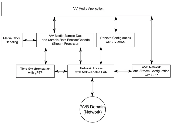
Figure 1. Example System Architecture

The functionality of the various blocks will be described in more detail later in this document. For illustration purposes, referring to Figure 1:

a) The A/V Media Application creates or consumes various forms of content – audio or video. The media application is responsible for managing stream reservations and creating and consuming AVB streaming data using the suggested facilities described in this document. Other product domains might replace this application with one that utilizes AVB for time-sensitive control data streams, but the rest of the system would remain largely the same.

(11)

b) AVB Network and Stream Configuration detects and modifies key AVB network parameters, advertises the presence of AVB streams, negotiates the allocation of AVB bandwidth, and notifies the media application of key events.

c) Time Synchronization establishes a local time reference which is coordinated with other AVB nodes. The service reports the quality of the time reference coordination, and provides translation services

between time measurements of other local clocks and the coordinated reference clock.

d) Media Clock Handling uses the distributed network clock maintained by Time Synchronization to synchronize other distinct clocks between AVB endpoints. Media clocks are generated by an independent programmable phase-lock loop (PLL) and provide the clocking for analog-to-digital or digital-to-analog converters (ADC/DAC).

e) AVB LAN provides accurate timestamps of time synchronization packet transmit and receive events, receives AVB streaming data traffic, or transmits AVB streaming data traffic consistent with the stream bandwidth reservation allocated by the AVB Network and Stream configuration module and the AVB forwarding and queuing rules.

f) The Stream Processor merges the various functions to encapsulate media data (such as samples and timestamps) for transmission via the AVB LAN block. It also receives data from the AVB LAN module and separates the media data for playback and clock recovery.

g) Remote Configuration enables advanced AVB device detection and configuration, as well as stream connection management facilities. Higher level protocols, such as Audio/Video Device Discovery, Enumeration, Connection Management and Control (AVDECC), are commonly use to coordinate the connection and operation of AVB devices within the network above and beyond low-level bandwidth allocation and streaming protocols. For example, common usages to connect an input to an output and modify the volume for playback map to AVDECC’s ability to identify all available nodes, instruct a listener (attached to a speaker) to connect to a specific talker stream (which could represent a specific microphone), and remotely modify playback parameters such as volume.

3.1. The A/V Media Application

For completeness, a description of common expected functions of media applications is included to frame the relevance of underlying services and APIs. The media application needs to manage the various media input and output devices, decide what streams to make available or access, and when to make the streams available. At a high level, the media application may manage live media or stored media. Live media refers to systems that use hardware for capturing or playing media in real-time, such as a hardware ADC/DAC or Codec. Live media AVB devices require media sample rate control, interface clock selection and configuration, a start/stop control and some form of DMA engine to access the samples, and specifically for AVB, time stamp of the media clock to a reference clock. In order to stream live media, AVB must associate media clock timestamps with specific samples captured or emitted. The media clock is then encoded into the stream, using a common network time as a timebase.

In the case of playback from stored media, such as a system to distribute stored music and pre-recorded announcements across a building, the media application could reasonably expect to implement rate control

(12)

functionality, media buffer management, and synthesizing timestamp information based on stored media clock information.

3.2. Time Synchronization

No two unadjusted oscillators run at precisely the same frequency. As a consequence, clocks based on these different oscillators do not agree on the time. This lack of a common time-base makes it impossible to play the same media sample(s) at the same time to two or more media output devices. Furthermore, if data is sourced by one system to be consumed at the same rate by another system, eventually the receiver data buffer will over-run or under-run depending upon which oscillator is faster.

The matching of one clock (as characterized by an oscillator) to another can be described by two terms,

syntonization and synchronization. Two clocks are said to be syntonized when their oscillators are precisely the same in frequency. In other words, they measure time passing at precisely the same rate. This is an essential property for media clocks.

Two clocks are said to be synchronized when they both agree precisely on what time it is at any moment. Their characteristic oscillators need not be syntonized to the same frequency, but they must agree precisely on the rate at which time passes even if one does not measure it as often as the other. Otherwise, their notions of what the current time is will begin to drift with respect to one another immediately after they are synchronized. The synchronization property is sometimes less important for media clocks, depending on whether phase alignment is required, but AVB can provide both syntonization and synchronization.

If probes are attached to media clock signals from two AVB devices that have syntonized and synchronized their clocks, an oscilloscope will show the two clock signals to be precisely matching in frequency and phase. This provides the foundation for synchronization of played media samples.

The AVB Time and Clock Synchronization services are based on a synchronized clock service in each device that can be used to syntonize and synchronize any number of media clocks between AVB devices. Each end node implements one or more Clocks. Each Clock is related to the other relevant Clocks, fundamentally referenced to a network time established by generalized Precision Time Protocol, described below. A Clock measurement can be translated to units of another Clock, and the Clock itself can be queried for its quality to determine stability, or possible error, of the clock itself.

3.2.1.Introduction to gPTP

To meet the above requirements, AVB adopts and extends an established protocol for time synchronization in the realms of industrial control and telecommunication: IEEE Std. 1588™-2008, also known as "Precision Time Protocol" (PTP). Although the AVB adaptation can be considered a profile of PTP, it is different enough to warrant its own mostly-independent standard: IEEE Std. 802.1AS™-2011, also known as "generalized Precision Time Protocol" (gPTP).

(13)

gPTP defines a single Domain, which is a group of interconnected devices that support running gPTP over every active link between them. This is a separate concept from an SRP Domain (described later). The gPTP Domain may be different to the SRP Domain and the set of devices which can be used for AVB is the intersection of these two domains. In practice, the two notions of Domain will describe the same set of devices and links in a well-configured AVB network.

One essential difference between PTP and gPTP with respect to the concept of Domain is that a gPTP Domain explicitly does not support links through network switches that do not participate in the protocol. This means that in an AVB network, all network switches between AVB endpoints must support gPTP (and the other AVB protocols as well).

The protocol implements the following actions:

 Determines domain eligibility

 Elects a grandmaster clock

 Determines network delay between peers

 Determines time-of-day offset between grandmaster and others

 Determines frequency offset between grandmaster and others

 Provides time-of-day and interval measurement services with respect to the grandmaster clock's time

There is a great deal more detail involved in each of those actions as well as in the algorithmic combination of their outputs to produce the effect of time synchronization.

3.2.2.gPTP Time and Application

gPTP time is represented in terms of an epoch as well as a positive offset from epoch. gPTP time can simultaneously represent the nanosecond-unit clocks commonly encountered in AVB systems, as well as approximately 8.9 million years elapsed time from epoch. gPTP’s Extended Timestamp is defined as a 48-bit seconds and 48-bit fractional nanoseconds field2, which represents the positive time with respect to an epoch in seconds and 2-16 nanoseconds.

Although epoch is formally referenced to 00:00:00 TAI, 1 January 19703, a grandmaster using an internal oscillator as its ‘timeSource’ can define the epoch in an arbitrary manner4. Some systems may default epoch to start from zero. With these devices, as the grand master role possibly transitions from one to another device, the gPTP epoch may change as a result (as not all devices may start simultaneously). Other devices may choose seemingly random epoch values which could make the most significant bits of the Extended Timestamp

relevant. For full compatibility, a gPTP service must internally maintain a 78-bit gPTP time representation.

2_{IEEE Std. 802.1AS™-2011, Clause 6.3.3.5} 3

IEEE Std. 802.1AS™-2011, Clause 8.2.2

4

(14)

gPTP clocks are rarely deliberately grossly modified, unless a new clock master is selected. Although they could be derived from and initially synchronized to a global time, after activation, the absolute value would not be arbitrarily adjusted to reflect time keeping conventions such as daylight savings time, leap-second, or related clock modification.

It is important to remember implementations fundamentally separate media time (and clocks) from gPTP time. Although in a controlled network, changes in the master clock are unlikely, gPTP is designed to tolerate changes of the network time grandmaster. A/V Media Applications must comprehend this behavior of gPTP.

For example, Talkers and Listeners exchange gPTP timestamps for synchronization of playback. AVDECC defines a control type to transport a gPTP timestamp. AVTP also defines a 32-bit avtp_timestamp field calculated from the 32 most significations bits of the 48 bit gPTP fractionalNanoseconds field and the low 2 bits of the gPTP seconds field. If the A/V Media Application detects the grand master has changed, resulting in a possible discontinuity in gPTP time while a stream is in progress, the Media Application can use the AVTP ‘timestamp uncertain’5 field to maintain playback despite possible changes resulting in different gPTP epochs.

3.2.3.gPTP Operation

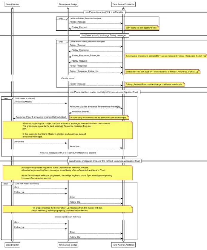
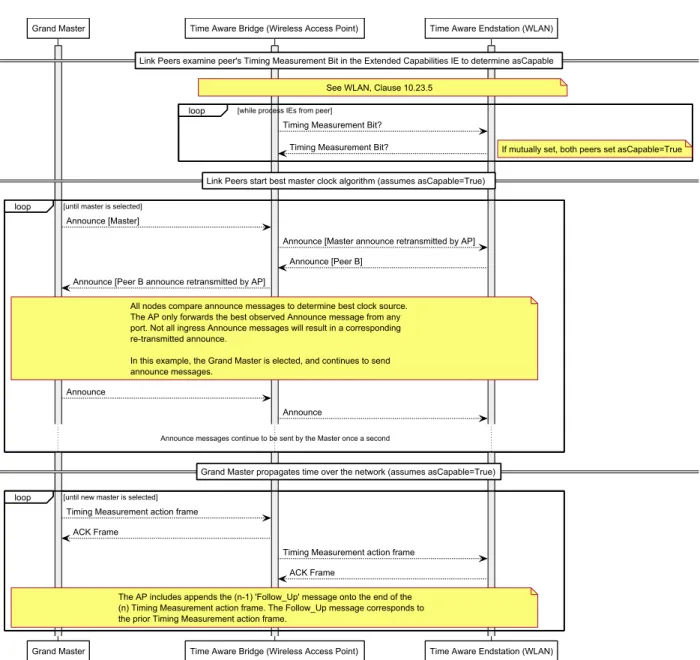
As illustrated in Figure 2 (for LAN) and Figure 3 (for WLAN), gPTP clock domain establishment occurs in four phases – determining whether the peer is capable of supporting gPTP (“asCapable”), determining the path delay and the rate of the peer’s clock (the neighborRateRatio), a best master clock master selection, and lastly to synchronize all nodes to the master time source.

5

(15)

(16)

Figure 3. Normal gPTP Clock Domain Establishment – WLAN-based

3.2.3.1.Determining Peer Capability

In the first phase, an end node begins transmitting messages in an attempt to detect whether the peer is capable of supporting gPTP. In the LAN case, this is accomplished by sending Pdelay messages and looking for a Pdelay Response message to be returned from the peer. In the WLAN case, each endpoint exchange Extended Capabilities Information Elements (IEs) with the ‘Timing Measurement’ capability bit set.

gPTP requires that all devices in the gPTP Domain support the protocol, and will not perform most protocol operations without first determining this capability. The mechanism used to discover peer capability is the Path Delay (Pdelay) measurement facility. If a peer responds to Pdelay requests within certain latency bounds, it is considered capable of participating in the protocol and the other protocol operations are enabled on the port

(17)

leading to the peer. If the peer does not respond, or if the latency of its response exceeds the bounds, the only gPTP operation that will continue is the attempt to determine peer capability with Pdelay requests.

3.2.3.2.Peer Rate Clock Determination

In the second phase, the end node calculates the link delay and a neighbor rate ratio. How this is done varies between LAN and WLAN. In the LAN case, repeated exchanges of Pdelay and Pdelay Response messages improve the estimation accuracy of the propagation delay, rate ratio of the peer, as well as track dynamic changes in rates (e.g. due to thermal changes). In the LAN case, path delays are not expected to vary because of physical changes. In the WLAN case, the path delay measurement and rate ratio is deferred to the clock

synchronization phase with the master. 3.2.3.3.Best Master Selection

In the third phase, the end-node sends announce messages which encode the default or administratively set clock quality parameters to determine which end-node will behave as the clock master for the clock domain. An administrator may set a priority on one end node over others to influence this selection process. The end-nodes may also have varying quality of reference clock source inputs – ranging from commodity crystal oscillators to GPS receiver inputs. Lastly, all things being equal, the MAC addresses of the various possible clock masters are compared.

At the initialization stage every Master-capable node starts by sending to its active ports Announce packets that include the clock parameters of its clock. Upon receipt of an Announce packet, a node compares the received clock parameters to its own and if the received parameters are better, then the node moves to the Slave state and stops sending Announce packets. When in Slave state the node compares incoming Announce packets to its currently chosen Master and if the new clock parameters are better than the current selected Master, the Slave transfers to the newly discovered Master clock. Eventually the best Master clock (BMC) is chosen. If the Slave fails to receive a Sync message within (typically) 5 sync intervals, the Slave times-out and moves to the Master state. It then resumes the process to select a new BMC.

The result of the Best Master Clock algorithm is a time-synchronization spanning-tree, in which all devices in the network derive their clocks via a single network path from the root clock, which is the Best Master Clock if one is available. Each non-leaf node is responsible for processing time synchronization data from its parent nodes and sending updated data to its children.

3.2.3.4.Clock synchronization

After a clock master has been chosen, the last phase begins with the clock master distribution of ‘Sync’ and ‘Follow_Up’ messages. On any link the port closest to the chosen grand master will in the ‘Master’ state,

(18)

whereas the other port (furthest from the grand master) – or ports as in shared media - would be in the ‘Slave’ state.6

The Master node periodically sends an event message – in this case a synchronization (Sync) message – with a default period of once per second. This synchronization message is deterministically time stamped by hardware as it leaves the interface, and that timestamp is communicated to slave devices. The timestamp is either sent via a Follow_Up message for LAN networks, or combined into a single Timing Measurement action frame for WLAN networks. The Sync and Follow_Up messages go to the node’s immediate children along the time

synchronization spanning tree path. These packets are addressed to special MAC addresses that are not forwarded by bridges, so each node in the tree must process incoming Sync packets and then emit new Sync packets to its children in the tree. WLAN networks combine the Sync and Follow_Up data into a single Timing Measurement action frame which carries the timing information from the current Sync frame and the timestamp of the previous Sync frame.

Each bridge increments a correction field (in the Follow_Up or Timing Measurement frame) to correct the computed time offset of the Sync message with the bridge residency time and the bridge-measured upstream path delay. The end (slave) node performs a similar calculation to add its own path delay correction to the bridge-supplied correction field. After applying these corrections, the end node is capable of computing a precise cumulative delay representing the time when the original Sync message was emitted by the clock master to the time when the Sync arrives at the end node.

When combining the correction field (from the bridge) with the local measurement of the peer link delay, the end node should convert any local hardware timestamps to gPTP time before calculating the peer link delay. The correction field can then be added to the peer link delay. As the bridge correction field is measured with the gPTP grand master clock, whereas the measured peer link delay timestamps are measured relative to a local reference clock (such as the LAN oscillator), the two clocks could materially differ in frequency to substantially affect accuracy.

Using several synchronization time stamps and path delay measurements, the Slave node can perform a linear best fit algorithm as described above to determine the rate ratio and the phase offset of its local clock to the advertised Master clock rate.

When using gPTP, the packets are sent to a gPTP reserved destination multicast MAC address–

01:80:C2:00:00:0E - using a Layer-2 (L2) encapsulation with the gPTP allocated Ethertype – 88-F7. Although this defined MAC address is a multicast address, the address falls within a bridge management reserved range and is not forwarded to other ports7. Note that many common residential and small office bridges do not obey the forwarding rules, and will replicate Nearest Bridge group address multicast frames to all other ports. Only a

6

IEEE Std. 802.1AS™-2011, Figure 10-10.

7

(19)

compliant switch will have this behavior of consuming Nearest Bridge group multicast frames. In this example, if the bridge has gPTP enabled, the bridge will generate new frames to transmit on all other egress ports. If gPTP is not enabled, new frames will not be generated and the behavior will appear to be suppressing frames. Implementers should be aware of implicit timing requirements of media dependent functions. For example, a bridge LAN port is said to be asCapable if the end node responds to Pdelay_Req (a request) with Pdelay_Resp (a response) and Pdelay_Resp_Follow_up. If the end node does not respond, bridges will declare the port not asCapable, and will not enable AVB functionality on the LAN port8.

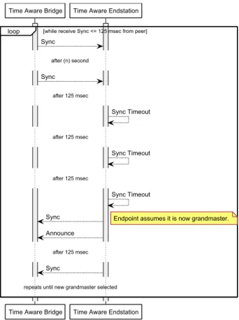
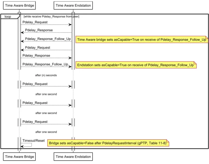
3.2.3.5.Error Conditions

Each of the various periodic message exchanges is a source of a possible error condition. The most likely error, illustrated in Figure 4, would be timing out receiving Sync messages from the Grand Master, indicating the master has disappeared, although Pdelay (Figure 5) and Announce (Figure 6) timeouts are also possible error conditions.

8

See IEEE Std. 802.1AS™-2011 Clause 12.3 and 13.4 for a discussion about the determination of asCapable. The original IEEE Std. 802.1AS™-2011 mandated a 10 millisecond response time (Annex B.2.3), although it was later relaxed by IEEE Std. 802.1AS™-Cor-1 (Clause 11.2.15.3). For maximum compatibility, end nodes should respond within 10 milliseconds or less, but a response delay can be as large as the Pdelay_Req message transmission interval (as long as the response arrives before the next Pdelay exchange).

(20)

(21)

(22)

Figure 6. Announce Timeout – Media Independent

3.2.4.Clock Fidelity

There are several methods to report the quality of the local gPTP time. Obviously, if the local node is the gPTP grandmaster, the problem reduces to reporting the gPTP time is perfectly “locked”. Hence, the question is how can slave mode devices best determine and report the fidelity of the recovered gPTP clock. Since the gPTP clock is used for clock recovery of other clocks such as media clocks, jitter in the gPTP clock will lead to jitter on derived clocks.

For software, reporting the error samples of the local clock relative to the gPTP clock as recovered by gPTP would suffice to indicate clock recovery quality. Error is defined as the delta in nanoseconds between a freshly computed grand master time on arrival of a Sync message (that being the corrected grand master time after applying correction factors and path delay estimates) versus the previous extrapolated local estimate of time referenced to the same local network timestamp value. The network timestamp of the Sync packet is computed using the prior gPTP estimate and again with the updated gPTP estimate. The difference between the two values is reported as the error. The gPTP service supports reporting at least the last eight (8) error samples.

(23)

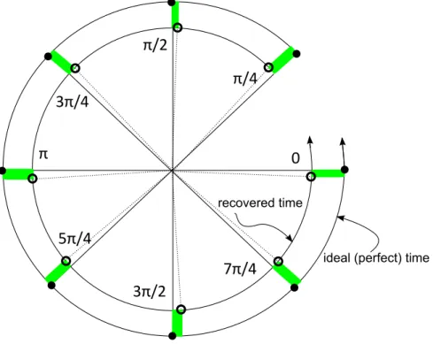
In Figure 7 below, time sweeps a full 2π radian every second (1 Hz), where the grand master is assumed by definition to be perfectly ideal, and any deviation or variability is caused by noise which could include

transmission jitter or quantization error from the grand master LAN interface, bridges or the end node itself. The end node samples, via the Sync message, the ideal time 8 times a second represented by the various π/4 intervals on the unit circle. Ideally, after correcting for bridge propagation delays and the local path delay, the Sync receive timestamp referenced to the local gPTP time should match exactly the master gPTP time. In other words, the Sync transmission from master to slave should appear instantaneous after applying appropriate corrections, and furthermore the local hardware timestamp on the Sync packet as received should translate to the same gPTP time using the previous gPTP estimate and the updated gPTP estimate.

In reality, there will be differences between the two times - the local gPTP may over or under estimate the rate of the gPTP time, as well as experience jitter from various sources. The green bars represent the sampling error observed by the end-node – again, both local quantization errors introduced by the local LAN interface, as well as errors introduced by the grand master and bridges. The width of the green bar is the observed error - the computed phase offset between the ideal gPTP time (outer ring) and the local recovered PTP time (inner ring). A variance calculation over (n) error samples can provide an indication how well the local gPTP subsystem is tracking the ideal time. The interpretation of the error variance is left to the application to determine fitness and suitability for use (as it may vary depending on application).

(24)

3.3. Media Clock Transformations

A media clock, sometimes called a word clock, is generally a signal used to synchronize various media sampling and playback devices to exchange media samples at a constant sampling rate. In the case of audio, the media clock is the digital sampling rate of the analog inputs.

The media clock controls the rate at which media samples flow from the source to the destination, typically called the sample rate. To meet fidelity requirements the sampling rate of the source and destination must be identical. This ensures that buffers and their associated latency can be small and bounded. It also eliminates the need for sample rate conversion and enables multiple device synchronization.

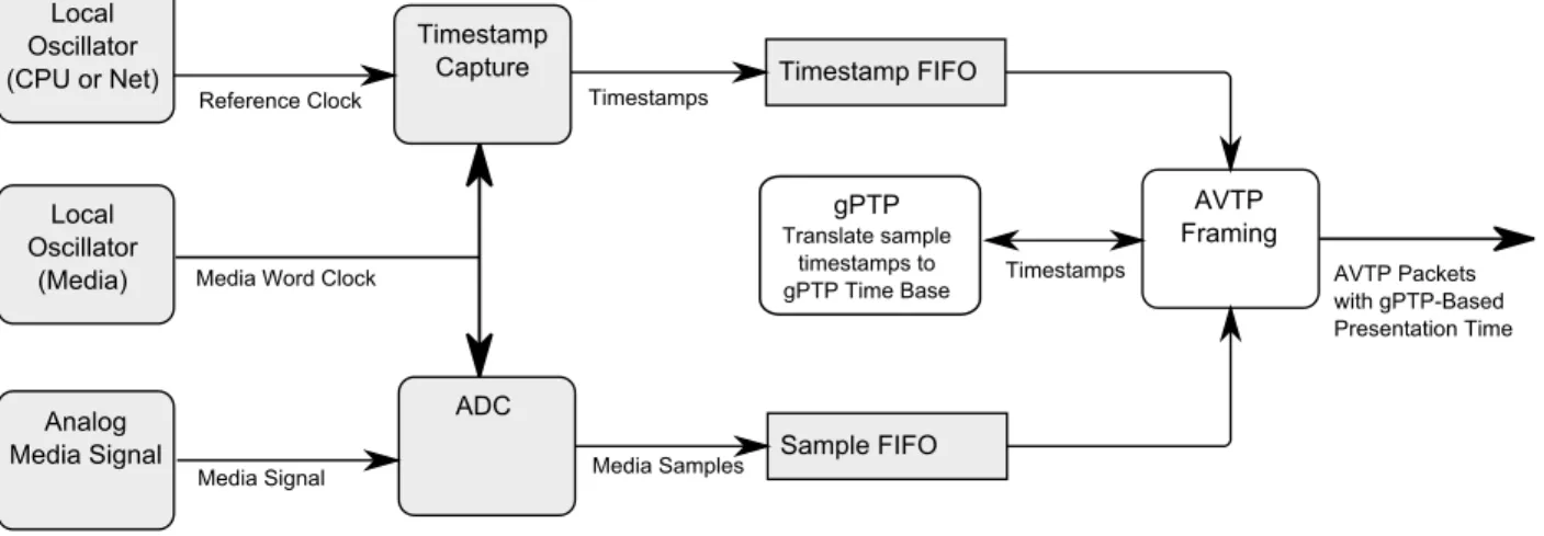
When an AVB Talker is sending media to an AVB Listener, a mechanism must be in place to guarantee that the media clocks between the two endpoints are synchronized. Audio/Video Transport Protocol (AVTP) defines streaming formats which contain an embedded media clock but it is possible to use other streaming formats which do not have an embedded media clock and provide a media clock through another mechanism. The media clock timestamps must be converted to a gPTP timebase by the Talker using the gPTP clock reference. See Figure 8 for an illustration. Similarly, all Listeners must be capable of recovering the media clock information, if

available, from the stream received from the Talker.

Figure 8. Simplified Talker Media Word Clock encoding

The mechanism used to embed the media clock, as defined in AVTP, uses the gPTP time as a reference for the Presentation Time Reference Planes. Figure 5.4 – Presentation Time Measurement Point - in the AVTP

specification shows ingress and presentation time reference planes that indicate the relative timing points for the media clock timestamps. As shown in Figure 8, the Talker for a media stream matches sample timestamps (translated to gPTP time) with the media samples produced at the time-stamped clock edge. The timestamps may be packaged along with their corresponding samples in the media transport stream according to the media transport protocol format.

(25)

gPTP provides a wall clock service based on Domain-wide clock synchronization. The single synchronized clock service of gPTP can be used to provide a service that recovers the media clock from any media stream. The underlying mechanism for this service is a procedure known as cross-time-stamping.

Cross time-stamping uses the gPTP time as a shared timebase to accurately measure the period of a local oscillator. A cross timestamp provides a cross reference between two clocks. A cross timestamp provides an instantaneous time reference in two time domains.

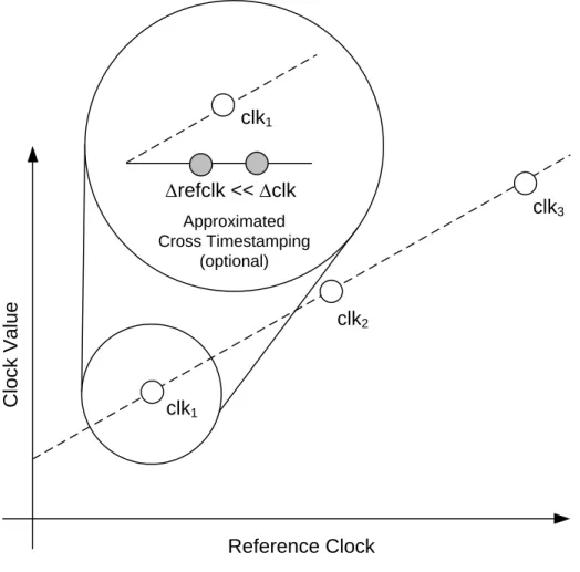
Figure 9 illustrates the general process of sampling a clock relative to another reference clock. The gPTP software typically performs a linear regression to fit the time stamp samples. In the diagram, the rate of ‘clk’ is sampled relative to a progression of a local reference clock ‘refclk’. From this information, the gPTP software stack then creates a linear equation to use as a time reference to scale a local clock to network time, where the scaling factor is the grandmaster frequency rate ratio, and the absolute time determined by calculation of the propagation delays of the grandmaster announced precise time.

In some implementations, the timestamp values may need to be approximated. A common example is when CPU-based timing features are used to sample a clock in software. In this case, two samples of the reference clock should be used to bracket the sampled clock value instead of just one. Again referring to Figure 9 as an example, ’clk’ is sampled, bracketed by two samples of ‘refclk’. The time delta between the two refclk samples is assumed to be minimized as to also minimize the error caused by the rate of change of clk.

(26)

Approximated Cross Timestamping (optional) Reference Clock C lo c k V a lu e Drefclk << Dclk clk1 clk2 clk3 clk1

Figure 9. Cross Timestamp Sampling

Highly integrated solutions may keep the LAN local clock synchronized with the network time rather than maintaining two or more clocks. However, keeping the network time separate from any one given network interface may be useful when implementing multi-port or multi-network systems. The gPTP software stack can also translate many other clock sources on the system – such as relating an audio device media clock time stamp to a CPU time stamp counter value in order to schedule sample delivery to occur precisely at the presentation time.

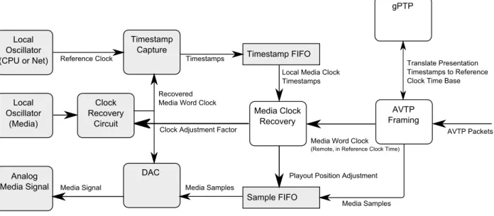
As shown in Figure 10, the Listener device extracts the cross-timestamps from the media transport stream data. The difference between two cross-timestamps is the amount of time, as measured by the gPTP clock, between the clock edges at which the corresponding samples were taken. Dividing the time interval between cross-timestamps by the number of samples generated between cross-cross-timestamps yields an estimate of the clock period of the source media clock. Continually performing this calculation and applying appropriate filtering techniques yields an accurate measurement of the source’s media clock period.

(27)

The Listener device performs a similar measurement of its own media clock, cross-timestamping it at regular intervals with the gPTP reference clock, and uses those measurements to derive the local media clock period. Since both media clocks are being measured with respect to the same "measuring stick" of gPTP time, the measured clock periods can be directly compared.

The difference between remote and local clocks is fed into a control mechanism (typically a combination of software and hardware) that adjusts the local media clock until it is syntonized and then synchronized with the remote media clock.

Figure 10. Example Listener Media Word Clock Recovery

For specific applications or engineered systems which implement point-to-point, or one-to-many Talker to Listener configurations, the Talker can supply the gPTP clock and media clock from the same reference. On the Listener, media clock recovery effectively becomes an output of the gPTP synchronization process. This solution can minimize product implementation cost by eliminating logic to scale gPTP time back to local reference clocks for the purpose of media clock recovery, but it comes at the cost of a great deal of AVB’s flexibility and

interoperability.

Many real world applications (a mixer for example) require a Listener to receive audio from multiple Talkers (many microphones for example). In these situations, a common media clock for all Talkers eliminates the need for sample rate conversion (SRC) operations inside the Listener. The implication is that some sort of “House Media Clock” equivalent for AVB is required. Although not formally part of the AVB specification suite, the simplest method of distributing a “House Media Clock” is via a designated AVB stream that contains the canonical media clocking information - any stream can be designated as the house clock reference stream. Any Talker device that can talk to a mixing device should also be capable of being a Listener so that it can Listen to “House Media Clock” AVTP packets and adjust its internal media clock to match the “House Media Clock”.

(28)

The house media clock implicitly requires all talkers which generate streams carrying media of whatever form to listen to the house media clock, and use the house media clock for all media generation. Listener-only devices (such as speakers) are not required to monitor the house media clock stream separately. Listeners can recover the media clock from the streams they consume directly.

3.4. AVB Network and Stream Configuration

An AVB system requires Talkers to declare media stream bandwidth requirements to the network prior to transmission on the network. End nodes and intermediate bridges use the Stream Reservation Protocol (SRP) to communicate these requirements and status information in the form of MRP attributes (MRP is the underlying protocol and state machine definition for SRP). AVB bridges process these attributes indicated by the Talker and Listener end nodes to the SRP domain of the AVB network. This overall Stream Reservation Protocol determines what resources to allocate to the various streams. Co-operative bandwidth allocation enables low latency packet transmission and meets the performance guarantee of preventing packet loss due to congestion.

A Talker does not begin transmission until it is notified that at least one or more Listeners have requested to receive the stream and the bridge(s) reports the bandwidth has been successfully allocated.

The following describes the primary building block objects – Domains and Streams - used with the API definition.

Domains exist within an AVB network to describe user priority and a default VLAN tag configuration for AVB traffic classes. Bridges use the user priority to categorize traffic into specific traffic classes – either Class A or Class B for AVB. All participating AVB endpoints are required to join the Domain they intend to stream data upon, such that an AVB bridge can determine the boundary of the AVB stream reservation domain. A talker is not required to stream on the default VLAN advertised by the Domain. A talker however must join a VLAN prior to streaming upon a given VLAN. Streams are identified by an AVB network unique stream ID, and have

attributes such as a unique destination multicast9 MAC address, the associated VLAN ID and user priority, the worst-case application network data payload size, the rate at which the stream will send such packets into the AVB network, a binary indication of stream rank among other streams (e.g. emergency announcement or normal), and lastly the maximum accumulated latency which represents the worst case latency the media data has been in flight (from the talker presentation plane).

Talkers create one or more Streams, and Listeners subscribe to receive one or more Streams. AVB bridge devices monitor the bandwidth requirements of the individual streams, and allocate bandwidth and resources as

9

IEEE Std. 802.1Q™-2011, Clause 35.2.2.83 only defines the use of multicast and locally administered addresses for stream destination addresses. Historically there was concern about multicast behavior on WLAN networks, suggesting use of locally administered unicast addresses, although AVB-compliant WLAN access points should comply with IEEE Std. 802.11aa™-2012 which addresses multicast behavior. When a unicast stream is removed, expected bridge behavior is undefined, and hence endpoints should avoid using unicast destination stream addresses for maximum compatibility.

(29)

needed (e.g. when a Listener subscribes) to ensure delivery of the Stream content. A Stream can be active or stopped depending on whether there are active Listeners subscribed to the Stream.

The traffic class associated with the Stream affects the interpretation of some of the Stream attributes. For example, a Class A Stream with a declared packet rate of ‘1’ indicates the Stream will produce at most one network frame every 125 microseconds, whereas a Class B Stream with a packet rate of ‘1’ indicates the Stream will produce at most one network frame every 250 microseconds. This is called the observation interval of the Class. Another side-effect of the Class definition affects the traffic shaping behavior of a FQTSS-compliant egress port – which is either the local LAN port of the Talker or intermediate AVB bridges. At the port level, traffic shaping behavior of egress ports is managed over the aggregate Class bandwidth summed over all Streams of the same Class.

Higher level protocols – such as AVDECC Connection Management Protocol (ACMP) - exist to manage the Talkers and Listeners themselves to create, listen and delete Streams within an AVB network.

3.5. Stream Processing

When clock synchronization has been achieved, AVB Domain parameters declared, stream bandwidth allocated and Listeners detected, a Talker may begin streaming onto the network. Prior to initiating a stream transmission, class bandwidth on the Talker is adjusted. A talker must limit both individual transmission rate for each stream and total transmission rate for each class10. Some implementations may depend solely on software-based pacing of the individual packets of a stream or shaping the overall traffic class shapers, whereas others may use

hardware-based traffic shapers to enforce the bandwidth requirements.

Individual Ethernet frames are generated by merging standard header information with dynamic media content and corresponding isochronous AVB presentation timestamps. Generated packets may not always contain the same number of samples. A Talker is not required to fully utilize reserved bandwidth on each and every interval. The situation arises because of the media packet format rules, which can result in packets of different sizes or a packet transmission rate which isn’t an integer multiple of the observation interval of the traffic class. For example – a Class (A) packet may be transmitted every 125 microsecond (8kHz), whereas the underlying media clock could be any of a number of frequencies (such as 44.1kHz and 48kHz). The AVTP presentation time is the time at which the defined sample within the AVTPDU crosses the Listener’s Presentation Time Reference Plane11. The presentation time is offset from the Talker’s Ingress Time Reference Plane by the network transit time which defaults to 2 milliseconds or 50 milliseconds depending on whether the stream is Class A or Class B.12 To reduce latency in engineered systems, Talker implementations may be configured to use an alternate transit time based on the maximum accumulated latency of potential listeners. The Talker Advertise Accumulated

10_{IEEE Std. 802.1Q™-2011, Clause 5.18, 34.6.1.} 11

IEEE Std. 1722™-2011, Clause 5.5.4

12

(30)

Latency is reported by SRP to the Listener13, and can be observed on the Listener via methods documented in AECP.

In practical Talker implementations that support multiple streams, care must be taken to submit and sequence the packets – perhaps in a round robin fashion - from the various streams onto the FTQSS shaper per-class queues. For example, as a hardware-based class shaper is adjusted, the class shaper may momentarily send more or less data on some existing streams belonging to that traffic class if the individual streams were not paced and interleaved correctly in the queue. This can cause over-runs or under-runs on receivers or within the bridged network itself.

The streaming functionality is typically implemented in the stream processor blocks described earlier. While the concept is general, the internal implementation details are very protocol and application specific. Some

examples include how the media clock control is integrated as well as how media samples are provided to the packets. These details are out of scope for this document. For the purposes of this document, at a minimum these modules must implement a configuration interface (which is protocol and application specific), a start interface to activate streaming (or prepare to receive a stream), and a stop interface (to gracefully stop a previously established stream resource).

3.6. AVB Remote Manageability and Control

Several important aspects of configuring and establishing streams are not covered by the low-level AVB related specifications. While this document will not go into detail, we do acknowledge a full design will implement a few additional features, such as resource allocation for streams as well as enumeration and control of device

capabilities. Of particular relevance, but not covered here, is the AVDECC Connection Management Protocol (ACMP), and AVDECC Enumeration and Control Protocol (AECP). ACMP and AECP together can be used to remotely start an AVB stream and constitutes a layer on top of the SRP interface outlined in this document. Open systems – those being integrated into notebook, desktop or workstations on standard high-volume operating systems for example – may implement interfaces to enumerate and enable/disable AVB functionality on LAN interfaces. Where multiple capable LAN interfaces exist, it may be required to configure each LAN interface individually, or alternatively (if attached to the same Layer-2 network), to configure the AVB components to prevent loopback effects (e.g. such as gPTP or MRP receiving copies of transmitted packets). Some form of network resource allocation – such as multicast address allocation for streams provided by MAC Address Acquisition Protocol (MAAP) or administrative allocation for example – is required to create streams, but outside of the scope of this document. Other higher level protocols would need to implement a similar method to allocate the multicast destination addresses required by SRP.

13

(31)

Talker and Listener devices may demonstrate enhanced flexibility – for instance, it is reasonable to expect a speaker device to be remotely configured to play back specific streams, and channels within given streams. For the purposes of this document, it is sufficient for controls to exist to create, start, stop and reclaim streams on an AVB subsystem without mandating how the streams will be used or mandating the details of how the stream content will be interpreted.

4. API Description Format

This section describes the format in which the API descriptions of the various AVB components will be presented. The approach taken follows a loosely object-oriented model, describing each interface in terms of objects and their data and operation members. This is merely for presentational clarity, as implementations need not follow an object-oriented approach so long as the essential protocol interfaces are available.

4.1. Objects

The objects are presented in a hierarchy that represents containment or composition; higher-level objects contain or are composed of lower-level ones. Each object described in the hierarchy represents a separately addressable active entity within the protocol or service.

4.2. Data Types

Passive data (i.e., not an active protocol entity) associated with the objects are represented via abstract data types, and these types are specified with respect to the meaning they carry within the protocol rather than the concrete representation they may take in an implementation. Simple types with short descriptions may be introduced in-line with data when their meaning is clear, but types requiring more explanation will be described with the most general enclosing object they are used within.

Simple types are used for values that can't be decomposed into a combination of simpler values. An integer or floating point value would be a simple type. An integer is assumed to be at least 32-bits by default unless otherwise specified. A floating point value is assumed to be 32-bit unless otherwise specified. Unless they require explanation beyond what is provided with the values they are associated with, they will not appear in the Data Types section. The descriptions will give sufficient information for implementations to choose a reasonable concrete implementation type.

Numeric types are examples of simple types that represent a numeric quantity. Depending on the needs of the API, a unit of measure may be associated with the type. A range restriction for the numeric values may also be associated with the type to indicate which numeric values are valid instances of the type.

Enumerated types are simple types that can take on one of a fixed set of non-numeric values. The possible values, represented as strings, are listed explicitly in the description of the type. An example would be an enumeration of the available AVB Classes – “Class ID:: Enumeration of Class A, Class B”.

(32)

Aggregate types are used for values that are composed of other values. They can be combined in several different ways. A common example is a structure type which describes values that have a fixed composition of sub-values that may be of various types. The same number and types of sub-values occur in the same order for each instance of the structure type. Structure types are sometimes known as "product types" or "record types". A variant type combines an enumerated type with a set of other types, at most one per element of the

enumeration. The associated types could be either simple types or aggregate types. Variant types are sometimes known as "sum types" or "tagged unions".

A collection type aggregates a number of values of the same type. Depending on the needs of the API, a more specific kind of collection might be specified, or bounds might be given for the allowable number of elements in the collection. More specific kinds of collections may include Sets, Lists, Arrays, Strings, Buffers, etc. Properties that distinguish specific kinds of collection may be described.

A collection type may be indicated by placing brackets after a type name, optionally with size bounds within the brackets. For example, Integer[1-10] would be a collection of Integers that ranges from 1 to 10 elements. For specific kinds of collections, a collection type may be indicated with <collection kind> of <type>. An optional size bound can be specified in brackets as with general collections.

4.3. Data Members

The data members of an object represent the data exposed by the object through its API. Together, the data members comprise the visible state of the object. They are listed along with their types and a description of their meaning and purpose within the system being described. Unless otherwise noted, data members are read-only via the API and are updated through operations or the internal working of the object.

Object state is described simply as data in order to leave the method by which it is accessed unspecified. Some implementations may follow a highly object-oriented approach with operations provided to read all state, while others may simply store data in pre-allocated tables that are exposed to the rest of the system.

4.4. Operation Members

Operations are the primary interaction points with objects. Each operation may take a fixed set of parameters, each of which is given with its type and a brief description of its meaning and purpose. The action associated with the operation is described as well.

Commands are operations that the user of the API initiates by invoking them with the required parameters. They may be used to request a service, invoke a protocol action, update some piece of object state, or some combination thereof.

(33)

Indications are operations that the object initiates and which present the associated parameters to the user of the API. They may be used to provide requested data, notify the user of some change in state, or report an error.

Commands and Indications are therefore discriminated by the primary direction of information flow that they facilitate. This is not meant to constrain the implementation to any particular mechanism: Commands might be implemented via function calls, placing messages in a queue, raising asynchronous events, etc. Indications might likewise be implemented via callback functions, polled message queues, asynchronous event listeners, etc.

4.5. API Dynamic Behavior Format

Interaction diagrams are presented after the descriptions of the APIs in order to illustrate common interaction scenarios. The diagrams will loosely follow the UML interaction diagram format. Participants in the diagram and their interaction arrows will be described as often as possible with the names of the objects and operations as presented in the API Description section.

Additional types of diagrams may be used to clarify, when appropriate, and their interpretation will be described as they are presented.

These are presented for the purpose of understanding typical interactions in the usage of the APIs, and are neither exhaustive in their coverage of possible cases nor normative in their description of interactions.

4.5.1.Successful operation cases

One or more diagrams may be presented to describe typical protocol behavior in successful cases; i.e. where no error or exceptional conditions arise. If more than one diagram is shown, they will show different valid

configurations of the participants in the protocol, and/or different patterns of interactions that lead to a successful case.

4.5.2.Exceptional operation cases

One or more diagrams may be presented to describe exceptional circumstances that may arise in the protocol operation and may be handled and reported by the protocol in question. These are not meant to specify higher-level error handling, but to describe what conditions may lead to any exceptional or error states described in the API Description.

5. Software Architecture

This section describes function prototype APIs, with associated commentary as to the usage and relevance. The function definitions themselves are purposefully left descriptive rather than call for a suggested function format with associated data type definitions. Details such as data types, error handling, notification methods – e.g. callback functions, event indications, etc. – are deliberately left to specific implementations to address in whatever manner is appropriate.

(34)

One key point not explicitly addressed is control, configuration and usage of multiple available physical network interfaces for AVB usage. The function descriptions in this section assume to operate on a single physical port context. The standards define the protocol operation on a per-port and per-endpoint basis.

5.1. gPTP

The gPTP subsystem must maintain and provide access to its local notion of the current gPTP time in a low-latency, low-jitter method. As the interface to operating-system device drivers vary greatly, a gPTP subsystem will generally require the following elements from the network interface:

 As necessary, access to all relevant clock sources, such as but not limited to the local LAN wall clock, cross time-stamped to a common system reference accessible to the PTP subsystem,

 Access to timestamps on received gPTP event frames,

 Access to timestamps on transmitted gPTP event frames.

Some highly integrated implementations may use a common reference clock for network packet timestamp and the gPTP reference clock. However, if the reference clock used for network packet timestamp is not the same as the gPTP reference clock, then the gPTP subsystem must have means to cross-timestamp and correlate the two clocks. For further motivation for this requirement, see the Precision Time Measurement (PTM) PCI-SIG ECN. Figure 11 implicitly assumes a simplified implementation based on a typical PC hardware architecture consisting of a LAN interface connected to a general purpose CPU. The diagram illustrates the resulting relationships between various Clock Objects to enable the gPTP subsystem to recover the network time from a remote Master node using locally available hardware clock sources. In this example, the gPTP subsystem uses the local CPU clock counter (‘TSC Clock Object’) to provide the gPTP time on-demand to client applications.

As Figure 11 illustrates, network packet timestamps are captured by the network interface, referenced to a network reference clock. The network reference clock itself is correlated to the CPU clock counter, enabling the gPTP subsystem to translate the PTP timestamp values from the network into CPU clock counter values (TSC). As additional timestamp Clock Times are provided with the PTP network packets, the gPTP subsystem calculates the Master AS-time rate related to the advance of the local CPU clock counter.

(35)

Figure 11. Example Clock System Diagram

The details of creating, enumerating and managing Clock instances are left to implementation discretion. A gPTP instance could range from a standalone subsystem providing services to applications, or used as a library or set of subroutines to a monolithic application.

Minimally, a “gPTP” clock would be created and maintained, with the underlying service consuming and producing gPTP event packets. Ancillary clock instances can be created as system-specific design requires. For instance, a media clock instance could be created to relate a media clock period to the gPTP time and vice versa.

5.1.1.Object Definitions

Object Description

Clock Object Clock Object:: Structure of Type:: Clock Type RateRatio:: Real number

PhaseOffset:: Integer in nanoseconds ClockSamples:: Clock Time[] samples

An object used to relate an incrementing counter with some arbitrary frequency and possible jitter to a common gPTP referenced global time. The clock frequency is determined by supplying a series of Clock Times and the gPTP subsystem is capable of calculating both the resultant frequency and jitter relative to the internally maintained gPTP time.

Although the times are all rooted ultimately to the gPTP time, a Clock Object can be indirectly related to gPTP time, where the units of supplied Clock Times are related to yet another initialized Clock Object.

(36)

although a common tradeoff to improve round off errors is to expose a parameter “RateRatioMinusOne”, as many of the rates are very close to the value 1.0. Subtracting ‘1.0’ makes a binary32 float value (defined in IEEE Std. 754™-2008) more stable for computation. For example, a clock that is 1 part per million fast relative to another clock could be represented as the number 1.000001 as a ratio, or could be represented as the value 0.000001 as the “RateRatioMinusOne”. 1.000001 represented as an IEEE float32 will have a 4.6 % error due to lack of enough mantissa bits, whereas the number 0.000001 will be accurate to the 14th decimal point.

5.1.2.Data Type Definitions

Data Type Description

Clock Time Clock Time:: 64 bit Integer

Sampled Value of a Clock Object. In practice, the Clock Time can be either an instantaneously latched value such as a sampled clock edge transition or an approximated value where a transition is detected by periodic sampling. Implementation-defined units, typically 64-bits of Clock Object units (interpretation defined by Clock Type).

Clock Type Clock Type:: Enumeration of gPTP, SysClock, LAN, MediaClock, …

System-specific enumeration of various clock sources available within an endpoint.

gPTP Clock Time gPTP Clock Time:: Structure of Seconds:: 64 bit Integer

FractionalNanoseconds::64 bit Integer

An expanded representation of the gPTP time exposing the 48-bit seconds and 48-bit FractionalNanoseconds fields of the Extended Timestamp of gPTP.

Grandmaster Status Grandmaster Status:: Enumeration of Available, Uncertain, New Election, Unavailable.

(37)

to get status, or to proactively notify clients.

In the simple case, if the local gPTP subsystem is the Grandmaster, the gPTP subsystem would report Available. As all nodes start out initially in the Grandmaster state until a best-master is chosen, this may be a transient state.

The Grandmaster can be Uncertain if for whatever reason the

synchronization packets are being intermittently dropped, or timestamp information not supplied.

A Grandmaster can have a New Election if a best-master clock algorithm executes and results in a change of the Grandmaster source. A client can also expect an Available status to be indicated.

The Grandmaster may also be Unavailable – in such cases when the best master clock algorithm hasn’t completed the initial selection, or the current Master fails and no end node does an announcement to reselect a master.

5.1.3.Data Member Definitions

Data Member Description

Slave-only mode Slave-only mode:: Boolean

In some usages, starting the gPTP subsystem in Slave-only mode enables faster and more reliable startup times by bypassing the requirement to execute the best master clock algorithm.

gPTP Rate Ratio gPTP Rate Ratio:: Real number scaling local clock source to master

A startup optimization involves saving and reloading rate ratios and path delays of the network from a prior system startup.

See the discussion above regarding the tradeoffs of a 64 bit representation versus a 32 bit representation, and methods to improve the representation. Path Delay Path Delay:: Integer in nanoseconds

(38)

A startup optimization involves saving and reloading path delays of the network from a prior system startup.

Neighbor Delay Neighbor Delay:: Integer in nanoseconds

The ability to adjust the neighbor delay enables applications to correct for fixed errors in the underlying packet timestamp hardware.

Discontinuity Threshold Discontinuity Threshold:: Integer in nanoseconds

A configurable threshold (in terms of jitter in RMS nanoseconds) on the gPTP subsystem to control when the gPTP subsystem indicates the selected clock master is unstable or unreliable.

5.1.4.Operation Definitions

Operation Direction Description Grandmaster

Change

Indication Grandmaster Change

Status:: Grandmaster Status

An event detected by the gPTP subsystem indicating to a gPTP client the gPTP service has selected a new Master for

synchronization.

Implementations must be tolerant of transient failures in the AVB network. One such transient event involves changes in the clock source being used as the master clock in the AVB network. In general, endpoints should continue to transfer media streams without interruption during a best master clock re-election.

When the master time disappears, the end nodes are said to enter into a free-wheel mode on the assumption that the previously compensated clocks will not rapidly drift from the