8.1 (Mostly) English Word Classes CHAPTER

CHAPTER

8

Part-of-Speech Tagging

Dionysius Thrax of Alexandria (c.100B.C.), or perhaps someone else (it was a long time ago), wrote a grammatical sketch of Greek (a “techn¯e”) that summarized the linguistic knowledge of his day. This work is the source of an astonishing proportion of modern linguistic vocabulary, including words likesyntax,diphthong,clitic, and

analogy. Also included are a description of eight parts of speech: noun, verb,

parts of speech

pronoun, preposition, adverb, conjunction, participle, and article. Although earlier scholars (including Aristotle as well as the Stoics) had their own lists of parts of speech, it was Thrax’s set of eight that became the basis for practically all subsequent part-of-speech descriptions of most European languages for the next 2000 years.

Schoolhouse Rock was a series of popular animated educational television clips from the 1970s. Its Grammar Rock sequence included songs about exactly 8 parts of speech, including the late great Bob Dorough’sConjunction Junction:

Conjunction Junction, what’s your function? Hooking up words and phrases and clauses...

Although the list of 8 was slightly modified from Thrax’s original, the astonishing durability of the parts of speech through two millennia is an indicator of both the importance and the transparency of their role in human language.1

Parts of speech (also known asPOS,word classes, orsyntactic categories) are

POS

useful because they reveal a lot about a word and its neighbors. Knowing whether a word is anounor averbtells us about likely neighboring words (nouns are pre-ceded by determiners and adjectives, verbs by nouns) and syntactic structure (nouns are generally part of noun phrases), making part-of-speech tagging a key aspect of parsing (Chapter 13). Parts of speech are useful features for labelingnamed entities like people or organizations ininformation extraction(Chapter 18), or for corefer-ence resolution (Chapter 22). A word’s part of speech can even play a role in speech recognition or synthesis, e.g., the wordcontentis pronouncedCONtentwhen it is a noun andconTENTwhen it is an adjective.

This chapter introduces parts of speech, and then introduces two algorithms for part-of-speech tagging, the task of assigning parts of speech to words. One is generative— Hidden Markov Model (HMM)—and one is discriminative—the Max-imum Entropy Markov Model (MEMM). Chapter 9 then introduces a third algorithm based on the recurrent neural network (RNN). All three have roughly equal perfor-mance but, as we’ll see, have different tradeoffs.

8.1

(Mostly) English Word Classes

Until now we have been using part-of-speech terms likenounandverbrather freely. In this section we give a more complete definition of these and other classes. While word classes do have semantic tendencies—adjectives, for example, often describe 1 _{Nonetheless, eight isn’t very many and, as we’ll see, recent tagsets have more.}

propertiesand nounspeople— parts of speech are traditionally defined instead based on syntactic and morphological function, grouping words that have similar neighbor-ing words (theirdistributionalproperties) or take similar affixes (their morpholog-ical properties).

Parts of speech can be divided into two broad supercategories:closed classtypes

closed class

andopen classtypes. Closed classes are those with relatively fixed membership,

open class

such as prepositions—new prepositions are rarely coined. By contrast, nouns and verbs are open classes—new nouns and verbs likeiPhoneorto faxare continually being created or borrowed. Any given speaker or corpus may have different open class words, but all speakers of a language, and sufficiently large corpora, likely share the set of closed class words. Closed class words are generallyfunction words

function word

likeof,it,and, oryou, which tend to be very short, occur frequently, and often have structuring uses in grammar.

Four major open classes occur in the languages of the world: nouns,verbs, adjectives, andadverbs. English has all four, although not every language does. The syntactic classnounincludes the words for most people, places, or things, but

noun

others as well. Nouns include concrete terms likeshipandchair, abstractions like

bandwidthandrelationship, and verb-like terms likepacingas inHis pacing to and fro became quite annoying. What defines a noun in English, then, are things like its ability to occur with determiners (a goat, its bandwidth, Plato’s Republic), to take possessives (IBM’s annual revenue), and for most but not all nouns to occur in the plural form (goats, abaci).

Open class nouns fall into two classes. Proper nouns, likeRegina,Colorado,

proper noun

andIBM, are names of specific persons or entities. In English, they generally aren’t preceded by articles (e.g.,the book is upstairs, butRegina is upstairs). In written English, proper nouns are usually capitalized. The other class,common nouns, are

common noun

divided in many languages, including English, intocount nounsandmass nouns.

count noun

mass noun Count nouns allow grammatical enumeration, occurring in both the singular and plu-ral (goat/goats, relationship/relationships) and they can be counted (one goat, two goats). Mass nouns are used when something is conceptualized as a homogeneous group. So words likesnow, salt, andcommunismare not counted (i.e.,*two snows

or*two communisms). Mass nouns can also appear without articles where singular count nouns cannot (Snow is whitebut not*Goat is white).

Verbsrefer to actions and processes, including main verbs likedraw,provide,

verb

andgo. English verbs have inflections (non-third-person-sg (eat), third-person-sg (eats), progressive (eating), past participle (eaten)). While many researchers believe that all human languages have the categories of noun and verb, others have argued that some languages, such as Riau Indonesian and Tongan, don’t even make this distinction (Broschart 1997;Evans 2000;Gil 2000) .

The third open class English form isadjectives, a class that includes many terms

adjective

for properties or qualities. Most languages have adjectives for the concepts of color (white, black), age (old, young), and value (good, bad), but there are languages without adjectives. In Korean, for example, the words corresponding to English adjectives act as a subclass of verbs, so what is in English an adjective “beautiful” acts in Korean like a verb meaning “to be beautiful”.

The final open class form,adverbs, is rather a hodge-podge in both form and

adverb

meaning. In the following all the italicized words are adverbs:

Actually, I ranhome extremely quickly yesterday

What coherence the class has semantically may be solely that each of these words can be viewed as modifying something (often verbs, hence the name

“ad-verb”, but also other adverbs and entire verb phrases).Directional adverbsor loca-tive adverbs(home,here,downhill) specify the direction or location of some action;

locative

degree adverbs(extremely,very,somewhat) specify the extent of some action,

pro-degree

cess, or property;manner adverbs(slowly,slinkily,delicately) describe the manner

manner

of some action or process; andtemporal adverbsdescribe the time that some

ac-temporal

tion or event took place (yesterday,Monday). Because of the heterogeneous nature of this class, some adverbs (e.g., temporal adverbs likeMonday) are tagged in some tagging schemes as nouns.

The closed classes differ more from language to language than do the open classes. Some of the important closed classes in English include:

prepositions: on, under, over, near, by, at, from, to, with particles: up, down, on, off, in, out, at, by

determiners: a, an, the

conjunctions: and, but, or, as, if, when pronouns: she, who, I, others

auxiliary verbs: can, may, should, are numerals: one, two, three, first, second, third

Prepositionsoccur before noun phrases. Semantically they often indicate spatial

preposition

or temporal relations, whether literal (on it,before then,by the house) or metaphor-ical (on time,with gusto,beside herself), but often indicate other relations as well, like marking the agent inHamlet was written by Shakespeare. Aparticleresembles

particle

a preposition or an adverb and is used in combination with a verb. Particles often have extended meanings that aren’t quite the same as the prepositions they resemble, as in the particleoverinshe turned the paper over.

A verb and a particle that act as a single syntactic and/or semantic unit are called aphrasal verb. The meaning of phrasal verbs is often problematically

non-phrasal verb

compositional—not predictable from the distinct meanings of the verb and the par-ticle. Thus,turn downmeans something like ‘reject’,rule out‘eliminate’,find out

‘discover’, andgo on‘continue’.

A closed class that occurs with nouns, often marking the beginning of a noun phrase, is thedeterminer. One small subtype of determiners is thearticle: English

determiner

article has three articles:a,an, andthe. Other determiners includethisandthat(this chap-ter,that page). Aandanmark a noun phrase as indefinite, whilethecan mark it as definite; definiteness is a discourse property (Chapter 23). Articles are quite fre-quent in English; indeed,theis the most frequently occurring word in most corpora of written English, andaandanare generally right behind.

Conjunctionsjoin two phrases, clauses, or sentences. Coordinating

conjunc-conjunctions

tions likeand,or, andbutjoin two elements of equal status. Subordinating conjunc-tions are used when one of the elements has some embedded status. For example,

that in“I thought that you might like some milk” is a subordinating conjunction that links the main clauseI thoughtwith the subordinate clauseyou might like some milk. This clause is called subordinate because this entire clause is the “content” of the main verbthought. Subordinating conjunctions likethatwhich link a verb to its argument in this way are also calledcomplementizers.

complementizer

Pronounsare forms that often act as a kind of shorthand for referring to some

pronoun

noun phrase or entity or event.Personal pronounsrefer to persons or entities (you,

personal

she,I,it,me, etc.). Possessive pronounsare forms of personal pronouns that

in-possessive

dicate either actual possession or more often just an abstract relation between the person and some object (my, your, his, her, its, one’s, our, their). Wh-pronouns

wh

complementizers (Frida, who married Diego. . .).

A closed class subtype of English verbs are theauxiliaryverbs.

Cross-linguist-auxiliary

ically, auxiliaries mark semantic features of a main verb: whether an action takes place in the present, past, or future (tense), whether it is completed (aspect), whether it is negated (polarity), and whether an action is necessary, possible, suggested, or desired (mood). English auxiliaries include thecopulaverbbe, the two verbsdoand

copula

have, along with their inflected forms, as well as a class ofmodal verbs.Beis called

modal

a copula because it connects subjects with certain kinds of predicate nominals and adjectives (He is a duck). The verbhavecan mark the perfect tenses (I have gone,I had gone), andbeis used as part of the passive (We were robbed) or progressive (We are leaving) constructions. Modals are used to mark the mood associated with the event depicted by the main verb:canindicates ability or possibility,maypermission or possibility,mustnecessity. There is also a modal use ofhave(e.g.,I have to go).

English also has many words of more or less unique function, including inter-jections(oh, hey, alas, uh, um),negatives(no, not),politeness markers(please, interjection

negative thank you),greetings(hello, goodbye), and the existentialthere(there are two on the table) among others. These classes may be distinguished or lumped together as interjections or adverbs depending on the purpose of the labeling.

8.2

The Penn Treebank Part-of-Speech Tagset

An important tagset for English is the 45-tag Penn Treebank tagset(Marcus et al.,

1993), shown in Fig. 8.1, which has been used to label many corpora. In such

labelings, parts of speech are generally represented by placing the tag after each word, delimited by a slash:

Tag Description Example Tag Description Example Tag Description Example

CC coordinating conjunction

and, but, or PDT predeterminer all, both VBP verb non-3sg

present

eat

CD cardinal number one, two POS possessive ending ’s VBZ verb 3sg pres eats

DT determiner a, the PRP personal pronoun I, you, he WDT wh-determ. which, that

EX existential ‘there’ there PRP$ possess. pronoun your, one’s WP wh-pronoun what, who

FW foreign word mea culpa RB adverb quickly WP$ wh-possess. whose

IN preposition/ subordin-conj

of, in, by RBR comparative

adverb

faster WRB wh-adverb how, where

JJ adjective yellow RBS superlatv. adverb fastest $ dollar sign $

JJR comparative adj bigger RP particle up, off # pound sign #

JJS superlative adj wildest SYM symbol +,%,& “ left quote ‘ or “

LS list item marker 1, 2, One TO “to” to ” right quote ’ or ”

MD modal can, should UH interjection ah, oops ( left paren [, (,{,< NN sing or mass noun llama VB verb base form eat ) right paren ], ),},>

NNS noun, plural llamas VBD verb past tense ate , comma ,

NNP proper noun, sing. IBM VBG verb gerund eating . sent-end punc . ! ? NNPS proper noun, plu. Carolinas VBN verb past part. eaten : sent-mid punc : ; ... –

-Figure 8.1 Penn Treebank part-of-speech tags (including punctuation).

(8.1) The/DT grand/JJ jury/NN commented/VBD on/IN a/DT number/NN of/IN other/JJ topics/NNS ./.

(8.3) Preliminary/JJ findings/NNS were/VBDreported/VBNin/IN today/NN ’s/POSNew/NNP England/NNP Journal/NNP of/IN Medicine/NNP ./. Example (8.1) shows the determinerstheanda, the adjectivesgrandandother, the common nouns jury,number, andtopics, and the past tense verbcommented. Example (8.2) shows the use of the EX tag to mark the existentialthereconstruction in English, and, for comparison, another use oftherewhich is tagged as an adverb (RB). Example (8.3) shows the segmentation of the possessive morpheme’s, and a passive construction, ‘were reported’, in whichreportedis tagged as a past participle (VBN). Note that since New England Journal of Medicine is a proper noun, the Treebank tagging chooses to mark each noun in it separately as NNP, including

journalandmedicine, which might otherwise be labeled as common nouns (NN). Corpora labeled with parts of speech are crucial training (and testing) sets for statistical tagging algorithms. Three main tagged corpora are consistently used for training and testing part-of-speech taggers for English. TheBrowncorpus is a

mil-Brown

lion words of samples from 500 written texts from different genres published in the United States in 1961. TheWSJcorpus contains a million words published in the

WSJ

Wall Street Journal in 1989. TheSwitchboardcorpus consists of 2 million words

Switchboard

of telephone conversations collected in 1990-1991. The corpora were created by running an automatic part-of-speech tagger on the texts and then human annotators hand-corrected each tag.

There are some minor differences in the tagsets used by the corpora. For example in the WSJ and Brown corpora, the single Penn tag TO is used for both the infinitive

to(I like to race) and the prepositionto(go to the store), while in Switchboard the tag TO is reserved for the infinitive use oftoand the preposition is tagged IN:

Well/UH ,/, I/PRP ,/, I/PRP want/VBPto/TOgo/VBto/INa/DT restaurant/NN Finally, there are some idiosyncracies inherent in any tagset. For example, be-cause the Penn 45 tags were collapsed from a larger 87-tag tagset, the original Brown tagset, some potentially useful distinctions were lost. The Penn tagset was designed for a treebank in which sentences were parsed, and so it leaves off syntactic information recoverable from the parse tree. Thus for example the Penn tag IN is used for both subordinating conjunctions likeif, when, unless, after:

after/INspending/VBG a/DT day/NN at/IN the/DT beach/NN and prepositions likein, on, after:

after/INsunrise/NN

Words are generally tokenized before tagging. The Penn Treebank and the British National Corpus split contractions and the’s-genitive from their stems:2

would/MD n’t/RB children/NNS ’s/POS

The Treebank tagset assumes that tokenization of multipart words like New Yorkis done at whitespace, thus tagging. a New York City firmasa/DT New/NNP York/NNP City/NNP firm/NN.

Another commonly used tagset, the Universal POS tag set of the Universal De-pendencies project(Nivre et al., 2016), is used when building systems that can tag many languages. See Section8.7.

8.3

Part-of-Speech Tagging

Part-of-speech taggingis the process of assigning a part-of-speech marker to each

part-of-speech tagging

word in an input text.3The input to a tagging algorithm is a sequence of (tokenized) words and a tagset, and the output is a sequence of tags, one per token.

Tagging is adisambiguationtask; words areambiguous—have more than one

ambiguous

possible part-of-speech—and the goal is to find the correct tag for the situation. For example,bookcan be a verb (book that flight) or a noun (hand me that book).

That can be a determiner (Does that flight serve dinner) or a complementizer (I thought that your flight was earlier). The goal of POS-tagging is toresolvethese

ambiguity resolution

ambiguities, choosing the proper tag for the context. How common is tag ambiguity? Fig.8.2shows that most word types (85-86%) are unambiguous (Janetis always NNP,funniestJJS, andhesitantlyRB). But the ambiguous words, though accounting for only 14-15% of the vocabulary, are very common words, and hence 55-67% of word tokens in running text are ambiguous.4

Types: WSJ Brown

Unambiguous (1 tag) 44,432 (86%) 45,799 (85%)

Ambiguous (2+ tags) 7,025 (14%) 8,050 (15%)

Tokens:

Unambiguous (1 tag) 577,421 (45%) 384,349 (33%) Ambiguous (2+ tags) 711,780 (55%) 786,646 (67%) Figure 8.2 Tag ambiguity for word types in Brown and WSJ, using Treebank-3 (45-tag) tagging. Punctuation were treated as words, and words were kept in their original case.

Some of the most ambiguous frequent words arethat,back,down,putandset; here are some examples of the 6 different parts of speech for the wordback:

earnings growth took aback/JJseat a small building in theback/NN

a clear majority of senatorsback/VBPthe bill Dave began toback/VBtoward the door enable the country to buyback/RPabout debt I was twenty-oneback/RBthen

Nonetheless, many words are easy to disambiguate, because their different tags aren’t equally likely. For example, a can be a determiner or the lettera, but the determiner sense is much more likely. This idea suggests a simplisticbaseline algo-rithm for part-of-speech tagging: given an ambiguous word, choose the tag which is most frequentin the training corpus. This is a key concept:

Most Frequent Class Baseline:Always compare a classifier against a baseline at least as good as the most frequent class baseline (assigning each token to the class it occurred in most often in the training set).

How good is this baseline? A standard way to measure the performance of part-of-speech taggers isaccuracy: the percentage of tags correctly labeled (matching

accuracy

3 _{Tags are also applied to punctuation, so tagging assumes tokenizing of commas, quotation marks, etc.,} and disambiguating end-of-sentence periods from periods inside words (e.g.,etc.).

4 _{Note the large differences across the two genres, especially in token frequency. Tags in the WSJ corpus} are less ambiguous; its focus on financial news leads to a more limited distribution of word usages than the diverse genres of the Brown corpus.

human labels on a test set). If we train on the WSJ training corpus and test on sec-tions 22-24 of the same corpus the most-frequent-tag baseline achieves an accuracy of 92.34%. By contrast, the state of the art in part-of-speech tagging on this dataset is around 97% tag accuracy, a performance that is achievable by most algorithms (HMMs, MEMMs, neural networks, rule-based algorithms). See Section 8.7 on other languages and genres.

8.4

HMM Part-of-Speech Tagging

In this section we introduce the use of the Hidden Markov Model for part-of-speech tagging. The HMM is asequence model. A sequence model orsequence

classi-sequence model

fieris a model whose job is to assign a label or class to each unit in a sequence, thus mapping a sequence of observations to a sequence of labels. An HMM is a probabilistic sequence model: given a sequence of units (words, letters, morphemes, sentences, whatever), it computes a probability distribution over possible sequences of labels and chooses the best label sequence.

8.4.1

Markov Chains

The HMM is based on augmenting the Markov chain. AMarkov chainis a model

Markov chain

that tells us something about the probabilities of sequences of random variables,

states, each of which can take on values from some set. These sets can be words, or tags, or symbols representing anything, for example the weather. A Markov chain makes a very strong assumption that if we want to predict the future in the sequence, all that matters is the current state. All the states before the current state have no im-pact on the future except via the current state. It’s as if to predict tomorrow’s weather you could examine today’s weather but you weren’t allowed to look at yesterday’s weather.

WARM3 HOT1

COLD2

.8

.6 .1

.1 .3

.6 .1

.1

.3

charming uniformly

are

.1

.4 _.5 .5

.5 .2

.6 .2

(a) (b)

Figure 8.3 A Markov chain for weather (a) and one for words (b), showing states and transitions. A start distributionπis required; settingπ= [0.1,0.7,0.2]for (a) would mean a

probability 0.7 of starting in state 2 (cold), probability 0.1 of starting in state 1 (hot), etc. More formally, consider a sequence of state variablesq1,q2, ...,qi. A Markov model embodies theMarkov assumptionon the probabilities of this sequence: that

Markov assumption

when predicting the future, the past doesn’t matter, only the present.

Markov Assumption: P(qi=a|q1...qi−1) =P(qi=a|qi−1) (8.4) Figure 8.3a shows a Markov chain for assigning a probability to a sequence of weather events, for which the vocabulary consists ofHOT,COLD, andWARM. The

states are represented as nodes in the graph, and the transitions, with their probabil-ities, as edges. The transitions are probabilities: the values of arcs leaving a given state must sum to 1. Figure8.3b shows a Markov chain for assigning a probability to a sequence of wordsw1...wn. This Markov chain should be familiar; in fact, it repre-sents a bigram language model, with each edge expressing the probabilityp(wi|wj)! Given the two models in Fig.8.3, we can assign a probability to any sequence from our vocabulary.

Formally, a Markov chain is specified by the following components:

Q=q1q2. . .qN a set ofNstates

A=a11a12. . .an1. . .ann atransition probability matrixA, eachai j represent-ing the probability of movrepresent-ing from stateito state j, s.t. Pn

j=1ai j=1 ∀i

π=π1,π2, ...,πN aninitial probability distributionover states. πiis the probability that the Markov chain will start in state i. Some states jmay haveπj=0, meaning that they cannot be initial states. Also,Pn

i=1πi=1

Before you go on, use the sample probabilities in Fig.8.3a (withπ= [0.1,0.7,0.2]) to compute the probability of each of the following sequences:

(8.5) hot hot hot hot (8.6) cold hot cold hot

What does the difference in these probabilities tell you about a real-world weather fact encoded in Fig.8.3a?

8.4.2

The Hidden Markov Model

A Markov chain is useful when we need to compute a probability for a sequence of observable events. In many cases, however, the events we are interested in are hidden: we don’t observe them directly. For example we don’t normally observe

hidden

part-of-speech tags in a text. Rather, we see words, and must infer the tags from the word sequence. We call the tagshiddenbecause they are not observed.

Ahidden Markov model(HMM) allows us to talk about bothobservedevents

Hidden Markov model

(like words that we see in the input) andhiddenevents (like part-of-speech tags) that we think of as causal factors in our probabilistic model. An HMM is specified by the following components:

Q=q1q2. . .qN a set ofNstates

A=a11. . .ai j. . .aNN atransition probability matrixA, eachai jrepresenting the probability of moving from stateito statej, s.t.PN

j=1ai j=1 ∀i

O=o1o2. . .oT a sequence ofT observations, each one drawn from a vocabularyV =

v1,v2, ...,vV

B=bi(ot) a sequence ofobservation likelihoods, also calledemission probabili-ties, each expressing the probability of an observationotbeing generated from a stateqi

π=π1,π2, ...,πN aninitial probability distributionover states. πiis the probability that the Markov chain will start in statei. Some states j may haveπj=0, meaning that they cannot be initial states. Also,Pn

A first-order hidden Markov model instantiates two simplifying assumptions. First, as with a first-order Markov chain, the probability of a particular state depends only on the previous state:

Markov Assumption: P(qi|q1...qi−1) =P(qi|qi−1) (8.7) Second, the probability of an output observationoidepends only on the state that produced the observationqiand not on any other states or any other observations:

Output Independence: P(oi|q1. . .qi, . . . ,qT,o1, . . . ,oi, . . . ,oT) =P(oi|qi) (8.8)

8.4.3

The components of an HMM tagger

Let’s start by looking at the pieces of an HMM tagger, and then we’ll see how to use it to tag. An HMM has two components, theAandBprobabilities.

TheAmatrix contains the tag transition probabilitiesP(ti|ti−1)which represent the probability of a tag occurring given the previous tag. For example, modal verbs likewillare very likely to be followed by a verb in the base form, a VB, likerace, so we expect this probability to be high. We compute the maximum likelihood estimate of this transition probability by counting, out of the times we see the first tag in a labeled corpus, how often the first tag is followed by the second:

P(ti|ti−1) =

C(ti−1,ti)

C(ti−1)

(8.9) In the WSJ corpus, for example, MD occurs 13124 times of which it is followed by VB 10471, for an MLE estimate of

P(V B|MD) =C(MD,V B) C(MD) =

10471

13124=.80 (8.10)

Let’s walk through an example, seeing how these probabilities are estimated and used in a sample tagging task, before we return to the algorithm for decoding.

In HMM tagging, the probabilities are estimated by counting on a tagged training corpus. For this example we’ll use the tagged WSJ corpus.

TheBemission probabilities,P(wi|ti), represent the probability, given a tag (say MD), that it will be associated with a given word (saywill). The MLE of the emis-sion probability is

P(wi|ti) =

C(ti,wi)

C(ti)

(8.11) Of the 13124 occurrences of MD in the WSJ corpus, it is associated withwill4046 times:

P(will|MD) =C(MD,will) C(MD) =

4046

13124 =.31 (8.12)

We saw this kind of Bayesian modeling in Chapter 4; recall that this likelihood term is not asking “which is the most likely tag for the wordwill?” That would be the posteriorP(MD|will). Instead,P(will|MD)answers the slightly counterintuitive question “If we were going to generate a MD, how likely is it that this modal would bewill?”

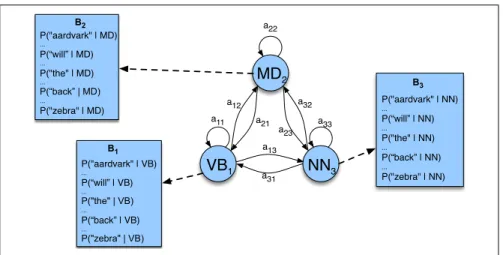
TheAtransition probabilities, and Bobservation likelihoods of the HMM are illustrated in Fig. 8.4for three states in an HMM part-of-speech tagger; the full tagger would have one state for each tag.

NN

VB

MD

P("aardvark" | NN)

...

P(“will” | NN)

...

P("the" | NN)

...

P(“back” | NN)

...

P("zebra" | NN)

B3

P("aardvark" | VB)

...

P(“will” | VB)

... P("the" | VB) ...

P(“back” | VB)

...

P("zebra" | VB)

B1

P("aardvark" | MD)

...

P(“will” | MD)

...

P("the" | MD)

...

P(“back” | MD) ...

P("zebra" | MD)

B2

Figure 8.4 An illustration of the two parts of an HMM representation: theAtransition probabilities used to compute the prior probability, and theBobservation likelihoods that are associated with each state, one likelihood for each possible observation word.

8.4.4

HMM tagging as decoding

For any model, such as an HMM, that contains hidden variables, the task of deter-mining the hidden variables sequence corresponding to the sequence of observations is calleddecoding. More formally,

decoding

Decoding: Given as input an HMMλ = (A,B)and a sequence of ob-servationsO=o1,o2, ...,oT, find the most probable sequence of states

Q=q1q2q3. . .qT.

For part-of-speech tagging, the goal of HMM decoding is to choose the tag se-quencet₁nthat is most probable given the observation sequence ofnwordswn₁:

ˆ

t₁n=argmax tn

1

P(t₁n|wn₁) (8.13)

The way we’ll do this in the HMM is to use Bayes’ rule to instead compute: ˆ

t₁n=argmax tn

1

P(wn₁|t₁n)P(t₁n) P(wn

1)

(8.14)

Furthermore, we simplify Eq.8.14by dropping the denominatorP(wn₁): ˆ

t₁n=argmax t₁n

P(wn₁|t₁n)P(t₁n) (8.15) HMM taggers make two further simplifying assumptions. The first is that the probability of a word appearing depends only on its own tag and is independent of neighboring words and tags:

P(wn₁|t₁n) ≈ n Y i=1

P(wi|ti) (8.16)

The second assumption, the bigramassumption, is that the probability of a tag is dependent only on the previous tag, rather than the entire tag sequence;

P(t₁n) ≈ n Y i=1

Plugging the simplifying assumptions from Eq. 8.16 and Eq. 8.17 into Eq. 8.15 results in the following equation for the most probable tag sequence from a bigram tagger:

ˆ

t₁n=argmax tn

1

P(t₁n|wn₁)≈argmax tn

1 n Y i=1

emission z }| { P(wi|ti)

transition z }| {

P(ti|ti−1) (8.18) The two parts of Eq.8.18correspond neatly to theBemission probabilityandA

transition probabilitythat we just defined above!

8.4.5

The Viterbi Algorithm

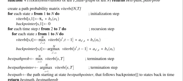
The decoding algorithm for HMMs is theViterbi algorithmshown in Fig.8.5. As

Viterbi algorithm

an instance ofdynamic programming, Viterbi resembles the dynamic program-mingminimum edit distancealgorithm of Chapter 2.

functionVITERBI(observationsof lenT,state-graphof lenN)returnsbest-path,path-prob

create a path probability matrixviterbi[N,T]

foreach statesfrom1toNdo ; initialization step

viterbi[s,1]←πs ∗bs(o1)

backpointer[s,1]←0

foreach time steptfrom2toTdo ; recursion step

foreach statesfrom1toNdo viterbi[s,t]←maxN

s0=1

viterbi[s0,t−1]∗as0_,s ∗b_s(o_t)

backpointer[s,t]←argmaxN

s0=1

viterbi[s0,t−1]∗as0_,s ∗bs(o_t)

bestpathprob←maxN

s=1

viterbi[s,T] ; termination step

bestpathpointer←argmaxN

s=1

viterbi[s,T] ; termination step

bestpath←the path starting at statebestpathpointer, that follows backpointer[] to states back in time

returnbestpath,bestpathprob

Figure 8.5 Viterbi algorithm for finding the optimal sequence of tags. Given an observation sequence and an

HMMλ= (A,B), the algorithm returns the state path through the HMM that assigns maximum likelihood to

the observation sequence.

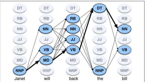
The Viterbi algorithm first sets up a probability matrix orlattice, with one col-umn for each observationotand one row for each state in the state graph. Each col-umn thus has a cell for each stateqi in the single combined automaton. Figure8.6 shows an intuition of this lattice for the sentenceJanet will back the bill.

Each cell of the lattice,vt(j), represents the probability that the HMM is in state

jafter seeing the firstt observations and passing through the most probable state sequenceq1, ...,qt−1, given the HMMλ. The value of each cellvt(j)is computed by recursively taking the most probable path that could lead us to this cell. Formally, each cell expresses the probability

vt(j) = max q1,...,qt−1

P(q1...qt−1,o1,o2. . .ot,qt=j|λ) (8.19)

We represent the most probable path by taking the maximum over all possible previous state sequences max

q1,...,qt−1

JJ

NNP NNP NNP

MD MD MD MD

VB VB

JJ JJ JJ

NN NN

RB RB

RB RB

DT DT DT DT

NNP

Janet will back the bill

NN

VB MD

NN

VB JJ RB

NNP DT

NN

VB

Figure 8.6 A sketch of the lattice forJanet will back the bill, showing the possible tags (qi) for each word and highlighting the path corresponding to the correct tag sequence through the hidden states. States (parts of speech) which have a zero probability of generating a particular word according to theBmatrix (such as the probability that a determiner DT will be realized

asJanet) are greyed out.

Viterbi fills each cell recursively. Given that we had already computed the probabil-ity of being in every state at timet−1, we compute the Viterbi probability by taking the most probable of the extensions of the paths that lead to the current cell. For a given stateqjat timet, the valuevt(j)is computed as

vt(j) = N max

i=1vt−1(i)ai jbj(ot) (8.20) The three factors that are multiplied in Eq.8.20for extending the previous paths to compute the Viterbi probability at timetare

vt−1(i) theprevious Viterbi path probabilityfrom the previous time step ai j thetransition probabilityfrom previous stateqito current stateqj

bj(ot) thestate observation likelihoodof the observation symbolot given the current state j

8.4.6

Working through an example

Let’s tag the sentenceJanet will back the bill; the goal is the correct series of tags (see also Fig.8.6):

(8.21) Janet/NNP will/MD back/VB the/DT bill/NN

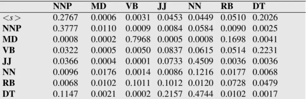
Let the HMM be defined by the two tables in Fig.8.7and Fig.8.8. Figure8.7 lists theai jprobabilities for transitioning between the hidden states (part-of-speech tags). Figure8.8expresses thebi(ot)probabilities, theobservationlikelihoods of words given tags. This table is (slightly simplified) from counts in the WSJ corpus. So the wordJanetonly appears as an NNP,backhas 4 possible parts of speech, and the wordthecan appear as a determiner or as an NNP (in titles like “Somewhere Over the Rainbow” all words are tagged as NNP).

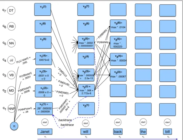
Figure8.9 shows a fleshed-out version of the sketch we saw in Fig. 8.6, the Viterbi lattice for computing the best hidden state sequence for the observation se-quenceJanet will back the bill.

NNP MD VB JJ NN RB DT

<s> 0.2767 0.0006 0.0031 0.0453 0.0449 0.0510 0.2026

NNP 0.3777 0.0110 0.0009 0.0084 0.0584 0.0090 0.0025

MD 0.0008 0.0002 0.7968 0.0005 0.0008 0.1698 0.0041

VB 0.0322 0.0005 0.0050 0.0837 0.0615 0.0514 0.2231

JJ 0.0366 0.0004 0.0001 0.0733 0.4509 0.0036 0.0036

NN 0.0096 0.0176 0.0014 0.0086 0.1216 0.0177 0.0068

RB 0.0068 0.0102 0.1011 0.1012 0.0120 0.0728 0.0479

DT 0.1147 0.0021 0.0002 0.2157 0.4744 0.0102 0.0017

Figure 8.7 TheAtransition probabilitiesP(ti|ti−1)computed from the WSJ corpus without

smoothing. Rows are labeled with the conditioning event; thusP(V B|MD)is 0.7968.

Janet will back the bill

NNP 0.000032 0 0 0.000048 0

MD 0 0.308431 0 0 0

VB 0 0.000028 0.000672 0 0.000028

JJ 0 0 0.000340 0 0

NN 0 0.000200 0.000223 0 0.002337

RB 0 0 0.010446 0 0

DT 0 0 0 0.506099 0

Figure 8.8 Observation likelihoodsBcomputed from the WSJ corpus without smoothing, simplified slightly.

There areN=5 state columns. We begin in column 1 (for the wordJanet) by setting the Viterbi value in each cell to the product of theπ transition probability (the start probability for that statei, which we get from the<s>entry of Fig.8.7), and the observation likelihood of the wordJanetgiven the tag for that cell. Most of the cells in the column are zero since the wordJanetcannot be any of those tags. The reader should find this in Fig.8.9.

Next, each cell in thewillcolumn gets updated. For each state, we compute the valueviterbi[s,t]by taking the maximum over the extensions of all the paths from the previous column that lead to the current cell according to Eq. 8.20. We have shown the values for the MD, VB, and NN cells. Each cell gets the max of the 7 values from the previous column, multiplied by the appropriate transition probabil-ity; as it happens in this case, most of them are zero from the previous column. The remaining value is multiplied by the relevant observation probability, and the (triv-ial) max is taken. In this case the final value, 2.772e-8, comes from the NNP state at the previous column. The reader should fill in the rest of the lattice in Fig.8.9and backtrace to see whether or not the Viterbi algorithm returns the gold state sequence NNP MD VB DT NN.

8.4.7

Extending the HMM Algorithm to Trigrams

Practical HMM taggers have a number of extensions of this simple model. One important missing feature is a wider tag context. In the tagger described above the probability of a tag depends only on the previous tag:

P(t₁n) ≈ n Y i=1

π

P(NNP|start) = .28

* P(MD|MD) = 0

* P(MD |NN P) .000 009* .01 = .9e-8 v1(2)=

.0006 x 0 = 0 v1(1) = .28* .000032 = .000009 t MD q2 q1 o1

Janet will bill

o2 o3

back

VB JJ

v1(3)= .0031 x 0

= 0 v1(4)= . 045*0=0

o4

* P(MD |VB) = 0 * P(MD

|JJ) = ₀ P(VB|start

) = .0031 P(JJ |sta

rt) = .045 backtrace q3 q4 the NN q5 RB q6 DT q7 v2(2) =

max * .308 = 2.772e-8 v2(5)= max * .0002

= .0000000001

v2(3)=

max * .000028 = 2.5e-13

v3(6)= max * .0104

v3(5)= max * . 000223 v3(4)= max * .00034

v3(3)= max * .00067 v1(5) v1(6) v1(7) v2(1) v2(4) v2(6) v2(7) backtrace * P(R B|N N) * P(NN|NN)

start _start start start start

o5

NNP P(MD|sta

rt) = .0006

Figure 8.9 The first few entries in the individual state columns for the Viterbi algorithm. Each cell keeps the probability of the best path so far and a pointer to the previous cell along that path. We have only filled out columns 1 and 2; to avoid clutter most cells with value 0 are left empty. The rest is left as an exercise for the reader. After the cells are filled in, backtracing from theendstate, we should be able to reconstruct the correct state sequence NNP MD VB DT NN.

In practice we use more of the history, letting the probability of a tag depend on the two previous tags:

P(t₁n) ≈ n Y i=1

P(ti|ti−1,ti−2) (8.23)

Extending the algorithm from bigram to trigram taggers gives a small (perhaps a half point) increase in performance, but conditioning on two previous tags instead of one requires a significant change to the Viterbi algorithm. For each cell, instead of taking a max over transitions from each cell in the previous column, we have to take a max over paths through the cells in the previous two columns, thus consideringN2

rather thanNhidden states at every observation.

In addition to increasing the context window, HMM taggers have a number of other advanced features. One is to let the tagger know the location of the end of the sentence by adding dependence on an end-of-sequence marker fortn+1. This gives the following equation for part-of-speech tagging:

ˆ

t₁n=argmax t₁n

P(t₁n|wn₁)≈argmax t₁n

" _n Y i=1

P(wi|ti)P(ti|ti−1,ti−2) #

In tagging any sentence with Eq.8.24, three of the tags used in the context will fall off the edge of the sentence, and hence will not match regular words. These tags,

t−1,t0, andtn+1, can all be set to be a single special ‘sentence boundary’ tag that is added to the tagset, which assumes sentences boundaries have already been marked. One problem with trigram taggers as instantiated in Eq.8.24 is data sparsity. Any particular sequence of tagsti−2,ti−1,ti that occurs in the test set may simply never have occurred in the training set. That means we cannot compute the tag trigram probability just by the maximum likelihood estimate from counts, following Eq.8.25:

P(ti|ti−1,ti−2) =

C(ti−2,ti−1,ti)

C(ti−2,ti−1)

(8.25) Just as we saw with language modeling, many of these counts will be zero in any training set, and we will incorrectly predict that a given tag sequence will never occur! What we need is a way to estimateP(ti|ti−1,ti−2)even if the sequence ti−2,ti−1,tinever occurs in the training data.

The standard approach to solving this problem is the same interpolation idea we saw in language modeling: estimate the probability by combining more robust, but weaker estimators. For example, if we’ve never seen the tag sequence PRP VB TO, and so can’t computeP(TO|PRP,VB) from this frequency, we still could rely on the bigram probabilityP(TO|VB), or even the unigram probabilityP(TO). The maximum likelihood estimation of each of these probabilities can be computed from a corpus with the following counts:

Trigrams Pˆ(ti|ti−1,ti−2) =

C(ti−2,ti−1,ti)

C(ti−2,ti−1)

(8.26)

Bigrams Pˆ(ti|ti−1) =

C(ti−1,ti)

C(ti−1)

(8.27) Unigrams Pˆ(ti) =

C(ti)

N (8.28)

The standard way to combine these three estimators to estimate the trigram probabil-ityP(ti|ti−1,ti−2)is via linear interpolation. We estimate the probabilityP(ti|ti−1ti−2) by a weighted sum of the unigram, bigram, and trigram probabilities:

P(ti|ti−1ti−2) = λ3Pˆ(ti|ti−1ti−2) +λ2Pˆ(ti|ti−1) +λ1Pˆ(ti) (8.29) We require λ1+λ2+λ3=1, ensuring that the resulting P is a probability distri-bution. Theλs are set by deleted interpolation(Jelinek and Mercer, 1980): we

deleted interpolation

successively delete each trigram from the training corpus and choose theλs so as to maximize the likelihood of the rest of the corpus. The deletion helps to set theλs in such a way as to generalize to unseen data and not overfit. Figure8.10gives a deleted interpolation algorithm for tag trigrams.

8.4.8

Beam Search

When the number of states grows very large, the vanilla Viterbi algorithm is slow. The complexity of the algorithm isO(N2T);N (the number of states) can be large for trigram taggers, which have to consider every previous pair of the 45 tags, re-sulting in 453=91,125 computations per column. Ncan be even larger for other applications of Viterbi, for example to decoding in neural networks, as we will see in future chapters.

functionDELETED-INTERPOLATION(corpus)returnsλ1,λ2,λ3

λ1,λ2,λ3←0

foreachtrigramt1,t2,t3withC(t1,t2,t3)>0

dependingon the maximum of the following three values

caseC(t1,t2,t3)−1

C(t1,t2)−1 : incrementλ3byC(t1,t2,t3) caseC(t2,t3)−1

C(t2)−1 : incrementλ2byC(t1,t2,t3) caseC(t3)−1

N−1 : incrementλ1byC(t1,t2,t3)

end end

normalizeλ1,λ2,λ3

returnλ1,λ2,λ3

Figure 8.10 The deleted interpolation algorithm for setting the weights for combining uni-gram, biuni-gram, and trigram tag probabilities. If the denominator is 0 for any case, we define the result of that case to be 0.Nis the number of tokens in the corpus. AfterBrants (2000).

One common solution to the complexity problem is the use ofbeam search

beam search

decoding. In beam search, instead of keeping the entire column of states at each time pointt, we just keep the best few hypothesis at that point. At timetthis requires computing the Viterbi score for each of theNcells, sorting the scores, and keeping only the best-scoring states. The rest are pruned out and not continued forward to timet+1.

One way to implement beam search is to keep a fixed number of states instead of allNcurrent states. Here thebeam widthβis a fixed number of states. Alternatively

beam width

β can be modeled as a fixed percentage of theNstates, or as a probability threshold. Figure8.11shows the search lattice using a beam width of 2 states.

JJ

NNP NNP NNP

MD MD MD MD

VB VB

JJ JJ JJ

NN NN

RB RB

RB RB

DT DT DT DT

NNP

Janet will back the bill

NN

VB MD

NN

VB JJ RB

NNP DT

NN

VB

Figure 8.11 A beam search version of Fig.8.6, showing a beam width of 2. At each time

t, all (non-zero) states are computed, but then they are sorted and only the best 2 states are propagated forward and the rest are pruned, shown in orange.

8.4.9

Unknown Words

know them Ishikawa Takuboku 1885–1912

To achieve high accuracy with part-of-speech taggers, it is also important to have a good model for dealing withunknown words. Proper names and acronyms are

unknown words

created very often, and even new common nouns and verbs enter the language at a surprising rate. One useful feature for distinguishing parts of speech is word shape: words starting with capital letters are likely to be proper nouns (NNP).

But the strongest source of information for guessing the part-of-speech of un-known words is morphology. Words that end in -sare likely to be plural nouns (NNS), words ending with-edtend to be past participles (VBN), words ending with

-ableadjectives (JJ), and so on. We store for each final letter sequence (for sim-plicity referred to as wordsuffixes) of up to 10 letters the statistics of the tag it was associated with in training. We are thus computing for each suffix of lengthi the probability of the tagtigiven the suffix letters (Samuelsson 1993,Brants 2000):

P(ti|ln−i+1. . .ln) (8.30)

Back-off is used to smooth these probabilities with successively shorter suffixes. Because unknown words are unlikely to be closed-class words like prepositions, suffix probabilities can be computed only for words whose training set frequency is ≤10, or only for open-class words. Separate suffix tries are kept for capitalized and uncapitalized words.

Finally, because Eq.8.30gives a posterior estimate p(ti|wi), we can compute the likelihood p(wi|ti)that HMMs require by using Bayesian inversion (i.e., using Bayes’ rule and computation of the two priorsP(ti)andP(ti|ln−i+1. . .ln)).

In addition to using capitalization information for unknown words,Brants (2000) also uses capitalization for known words by adding a capitalization feature to each tag. Thus, instead of computingP(ti|ti−1,ti−2)as in Eq.8.26, the algorithm com-putes the probabilityP(ti,ci|ti−1,ci−1,ti−2,ci−2). This is equivalent to having a cap-italized and uncapcap-italized version of each tag, doubling the size of the tagset.

Combining all these features, a trigram HMM like that ofBrants (2000)has a tagging accuracy of 96.7% on the Penn Treebank, perhaps just slightly below the performance of the best MEMM and neural taggers.

8.5

Maximum Entropy Markov Models

While an HMM can achieve very high accuracy, we saw that it requires a number of architectural innovations to deal with unknown words, backoff, suffixes, and so on. It would be so much easier if we could add arbitrary features directly into the model in a clean way, but that’s hard for generative models like HMMs. Luckily, we’ve already seen a model for doing this: the logistic regression model of Chapter 5! But logistic regression isn’t a sequence model; it assigns a class to a single observation. However, we could turn logistic regression into a discriminative sequence model simply by running it on successive words, using the class assigned to the prior word

as a feature in the classification of the next word. When we apply logistic regression in this way, it’s called themaximum entropy Markov modelorMEMM.5

MEMM

Let the sequence of words beW =wn₁and the sequence of tagsT =t₁n. In an HMM to compute the best tag sequence that maximizesP(T|W)we rely on Bayes’ rule and the likelihoodP(W|T):

ˆ

T = argmax

T

P(T|W)

= argmax

T

P(W|T)P(T)

= argmax

T Y

i

P(wordi|tagi) Y

i

P(tag_i|tag_i−1) (8.31)

In an MEMM, by contrast, we compute the posteriorP(T|W)directly, training it to discriminate among the possible tag sequences:

ˆ

T = argmax

T

P(T|W)

= argmax

T Y

i

P(ti|wi,ti−1) (8.32)

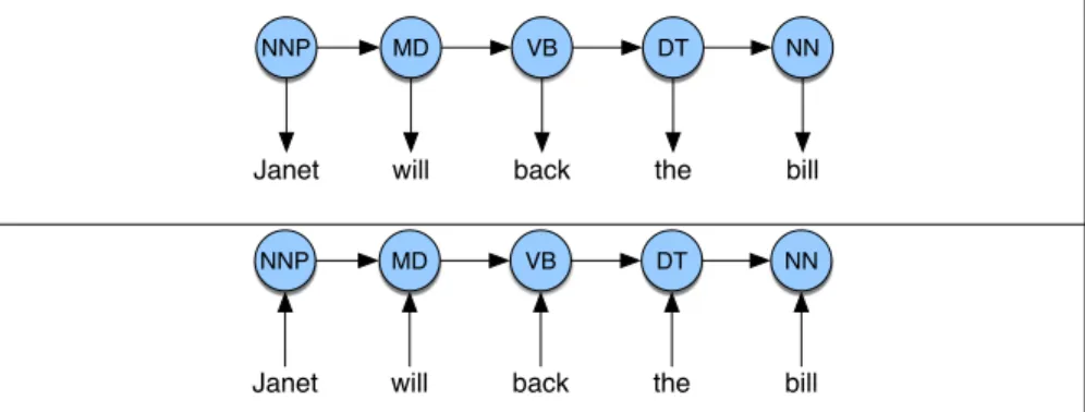
Consider tagging just one word. A multinomial logistic regression classifier could compute the single probabilityP(ti|wi,ti−1)in a different way than an HMM. Fig.8.12 shows the intuition of the difference via the direction of the arrows; HMMs compute likelihood (observation word conditioned on tags) but MEMMs compute posterior (tags conditioned on observation words).

will

MD VB DT NN

Janet back the bill

NNP

will

MD VB DT NN

Janet back the bill

NNP

Figure 8.12 A schematic view of the HMM (top) and MEMM (bottom) representation of the probability computation for the correct sequence of tags for thebacksentence. The HMM computes the likelihood of the observation given the hidden state, while the MEMM computes the posterior of each state, conditioned on the previous state and current observation.

8.5.1

Features in a MEMM

Of course we don’t build MEMMs that condition just on wiandti−1. The reason to use a discriminative sequence model is that it’s easier to incorporate a lot of fea-tures.6Figure8.13shows a graphical intuition of some of these additional features. 5 _{‘Maximum entropy model’ is an outdated name for logistic regression; see the history section.} 6 _{Because in HMMs all computation is based on the two probabilitiesP(tag|tag)andP(word|tag), if} we want to include some source of knowledge into the tagging process, we must find a way to encode the knowledge into one of these two probabilities. Each time we add a feature we have to do a lot of complicated conditioning which gets harder and harder as we have more and more such features.

will

MD VB

Janet back the bill

NNP

<s>

wi wi+1

wi-1 ti-1 ti-2

wi-2

Figure 8.13 An MEMM for part-of-speech tagging showing the ability to condition on more features.

A basic MEMM part-of-speech tagger conditions on the observation word it-self, neighboring words, and previous tags, and various combinations, using feature templateslike the following:

templates

hti,wi−2i,hti,wi−1i,hti,wii,hti,wi+1i,hti,wi+2i hti,ti−1i,hti,ti−2,ti−1i,

hti,ti−1,wii,hti,wi−1,wiihti,wi,wi+1i, (8.33)

Recall from Chapter 5 that feature templates are used to automatically populate the set of features from every instance in the training and test set. Thus our example

Janet/NNP will/MD back/VB the/DT bill/NN, whenwiis the wordback, would gen-erate the following features:

ti= VB andwi−2= Janet ti= VB andwi−1= will ti= VB andwi= back

ti= VB andwi+1= the ti= VB andwi+2= bill ti= VB andti−1= MD

ti= VB andti−1= MD andti−2= NNP ti= VB andwi= back andwi+1= the

Also necessary are features to deal with unknown words, expressing properties of the word’s spelling or shape:

wicontains a particular prefix (from all prefixes of length≤4)

wicontains a particular suffix (from all suffixes of length≤4)

wicontains a number

wicontains an upper-case letter

wicontains a hyphen

wiis all upper case

wi’s word shape

wi’s short word shape

wiis upper case and has a digit and a dash (likeCFC-12)

wiis upper case and followed within 3 words by Co., Inc., etc.

Word shapefeatures are used to represent the abstract letter pattern of the word

word shape

by mapping lower-case letters to ‘x’, upper-case to ‘X’, numbers to ’d’, and retaining punctuation. Thus for example I.M.F would map to X.X.X. and DC10-30 would map to XXdd-dd. A second class of shorter word shape features is also used. In these features consecutive character types are removed, so DC10-30 would be mapped to Xd-d but I.M.F would still map to X.X.X. For example the wordwell-dressedwould generate the following non-zero valued feature values:

prefix(wi) =w prefix(wi) =we prefix(wi) =wel prefix(wi) =well suffix(wi) =ssed suffix(wi) =sed suffix(wi) =ed suffix(wi) =d has-hyphen(wi)

word-shape(wi) =xxxx-xxxxxxx short-word-shape(wi) =x-x

Features for known words, like the templates in Eq.8.33, are computed for every word seen in the training set. The unknown word features can also be computed for all words in training, or only on training words whose frequency is below some threshold. The result of the known-word templates and word-signature features is a very large set of features. Generally a feature cutoff is used in which features are thrown out if they have count<5 in the training set.

8.5.2

Decoding and Training MEMMs

The most likely sequence of tags is then computed by combining these features of the input wordwi, its neighbors withinlwordswi+l_i−l, and the previousktagst

i−1 i−k as follows (usingθto refer to feature weights instead ofwto avoid the confusion with

wmeaning words): ˆ

T = argmax

T

P(T|W)

= argmax

T Y

i

P(ti|wi+l_i−l,t i−1 i−k)

= argmax

T Y

i

exp  

X j

θjfj(ti,wi+l_i−l,t i−1 i−k)

 

X t0_∈tagset

exp  

X j

θjfj(t0,wi+l_i−l,t i−1 i−k)

 

(8.34)

How should we decode to find this optimal tag sequence ˆT? The simplest way to turn logistic regression into a sequence model is to build a local classifier that classifies each word left to right, making a hard classification on the first word in the sentence, then a hard decision on the second word, and so on. This is called a greedydecoding algorithm, because we greedily choose the best tag for each word,

greedy

as shown in Fig.8.14.

functionGREEDYSEQUENCEDECODING(words W, model P)returnstag sequence T

fori= 1tolength(W)

ˆ

ti = argmax t0_∈T

P(t0|w_ii₋+l_l,t_ii₋−_k1)

Figure 8.14 In greedy decoding we simply run the classifier on each token, left to right, each time making a hard decision about which is the best tag.

The problem with the greedy algorithm is that by making a hard decision on each word before moving on to the next word, the classifier can’t use evidence from future decisions. Although the greedy algorithm is very fast, and occasionally has sufficient accuracy to be useful, in general the hard decision causes too great a drop in performance, and we don’t use it.

Instead we decode an MEMM with theViterbialgorithm just as with the HMM,

Viterbi

finding the sequence of part-of-speech tags that is optimal for the whole sentence. For example, assume that our MEMM is only conditioning on the previous tag

ti−1and observed word wi. Concretely, this involves filling an N×T array with the appropriate values forP(ti|ti−1,wi), maintaining backpointers as we proceed. As with HMM Viterbi, when the table is filled, we simply follow pointers back from the maximum value in the final column to retrieve the desired set of labels. The requisite changes from the HMM-style application of Viterbi have to do only with how we fill each cell. Recall from Eq.8.20that the recursive step of the Viterbi equation computes the Viterbi value of timetfor state jas

vt(j) = N max

i=1 vt−1(i)ai jbj(ot); 1≤ j≤N,1<t≤T (8.35) which is the HMM implementation of

vt(j) = N max

i=1 vt−1(i)P(sj|si)P(ot|sj) 1≤j≤N,1<t≤T (8.36) The MEMM requires only a slight change to this latter formula, replacing theaand

bprior and likelihood probabilities with the direct posterior:

vt(j) = N max

i=1 vt−1(i)P(sj|si,ot) 1≤j≤N,1<t≤T (8.37) Learning in MEMMs relies on the same supervised learning algorithms we presented for logistic regression. Given a sequence of observations, feature functions, and cor-responding hidden states, we use gradient descent to train the weights to maximize the log-likelihood of the training corpus.

8.6

Bidirectionality

The one problem with the MEMM and HMM models as presented is that they are exclusively run left-to-right. While the Viterbi algorithm still allows present deci-sions to be influenced indirectly by future decideci-sions, it would help even more if a decision about wordwicould directly use information about future tagsti+1andti+2. Adding bidirectionality has another useful advantage. MEMMs have a theoret-ical weakness, referred to alternatively as thelabel biasorobservation bias

prob-label bias observation

bias lem (Lafferty et al. 2001, Toutanova et al. 2003). These are names for situations

when one source of information is ignored because it isexplained awayby another source. Consider an example fromToutanova et al. (2003), the sequencewill/NN to/TO fight/VB. The tag TO is often preceded by NN but rarely by modals (MD), and so that tendency should help predict the correct NN tag forwill. But the previ-ous transitionP(twill|hsi)prefers the modal, and becauseP(T O|to,twill)is so close to 1 regardless oftwill the model cannot make use of the transition probability and incorrectly chooses MD. The strong information thattomust have the tag TO has ex-plained awaythe presence of TO and so the model doesn’t learn the importance of

the previous NN tag for predicting TO. Bidirectionality helps the model by making the link between TO available when tagging the NN.

One way to implement bidirectionality is to switch to a more powerful model called a conditional random fieldor CRF. The CRF is an undirected graphical

CRF

model, which means that it’s not computing a probability for each tag at each time step. Instead, at each time step the CRF computes log-linear functions over aclique, a set of relevant features. Unlike for an MEMM, these might include output features of words in future time steps. The probability of the best sequence is similarly computed by the Viterbi algorithm. Because a CRF normalizes probabilities over all tag sequences, rather than over all the tags at an individual timet, training requires computing the sum over all possible labelings, which makes CRF training quite slow. Simpler methods can also be used; the Stanford taggeruses a bidirectional

Stanford tagger

version of the MEMM called a cyclic dependency network(Toutanova et al., 2003). Alternatively, any sequence model can be turned into a bidirectional model by using multiple passes. For example, the first pass would use only part-of-speech features from already-disambiguated words on the left. In the second pass, tags for all words, including those on the right, can be used. Alternately, the tagger can be run twice, once left-to-right and once right-to-left. In greedy decoding, for each word the classifier chooses the highest-scoring of the tags assigned by the left-to-right and right-to-left classifier. In Viterbi decoding, the classifier chooses the higher scoring of the two sequences (left-to-right or right-to-left). These bidirectional models lead directly into the bi-LSTM models that we will introduce in Chapter 9 as a standard neural sequence model.

8.7

Part-of-Speech Tagging for Morphological Rich

Lan-guages

Augmentations to tagging algorithms become necessary when dealing with lan-guages with rich morphology like Czech, Hungarian and Turkish.

These productive word-formation processes result in a large vocabulary for these languages: a 250,000 word token corpus of Hungarian has more than twice as many word types as a similarly sized corpus of English(Oravecz and Dienes, 2002), while a 10 million word token corpus of Turkish contains four times as many word types as a similarly sized English corpus (Hakkani-T¨ur et al., 2002). Large vocabular-ies mean many unknown words, and these unknown words cause significant per-formance degradations in a wide variety of languages (including Czech, Slovene, Estonian, and Romanian)(Hajiˇc, 2000).

Highly inflectional languages also have much more information than English coded in word morphology, likecase(nominative, accusative, genitive) orgender (masculine, feminine). Because this information is important for tasks like pars-ing and coreference resolution, part-of-speech taggers for morphologically rich lan-guages need to label words with case and gender information. Tagsets for morpho-logically rich languages are therefore sequences of morphological tags rather than a single primitive tag. Here’s a Turkish example, in which the wordizinhas three pos-sible morphological/part-of-speech tags and meanings(Hakkani-T¨ur et al., 2002):

1. Yerdekiizintemizlenmesi gerek. iz +Noun+A3sg+Pnon+Gen

The traceon the floor should be cleaned.

Yourfingerprintis left on (it).

3. Ic¸eri girmek ic¸inizinalman gerekiyor. izin +Noun+A3sg+Pnon+Nom You needpermissionto enter.

Using a morphological parse sequence likeNoun+A3sg+Pnon+Genas the part-of-speech tag greatly increases the number of parts of speech, and so tagsets can be 4 to 10 times larger than the 50–100 tags we have seen for English. With such large tagsets, each word needs to be morphologically analyzed to generate the list of possible morphological tag sequences (part-of-speech tags) for the word. The role of the tagger is then to disambiguate among these tags. This method also helps with unknown words since morphological parsers can accept unknown stems and still segment the affixes properly.

For non-word-space languages like Chinese, word segmentation (Chapter 2) is either applied before tagging or done jointly. Although Chinese words are on aver-age very short (around 2.4 characters per unknown word compared with 7.7 for En-glish) the problem of unknown words is still large. While English unknown words tend to be proper nouns in Chinese the majority of unknown words are common nouns and verbs because of extensive compounding. Tagging models for Chinese use similar unknown word features to English, including character prefix and suf-fix features, as well as novel features like theradicalsof each character in a word.

(Tseng et al., 2005).

A standard for multilingual tagging is the Universal POS tag set of the Universal Dependencies project, which contains 16 tags plus a wide variety of features that can be added to them to create a large tagset for any language(Nivre et al., 2016).

8.8

Summary

This chapter introducedparts of speechandpart-of-speech tagging:

• Languages generally have a small set ofclosed classwords that are highly frequent, ambiguous, and act asfunction words, andopen-classwords like nouns,verbs,adjectives. Various part-of-speechtagsetsexist, of between 40 and 200 tags.

• Part-of-speech taggingis the process of assigning a part-of-speech label to each of a sequence of words.

• Two common approaches tosequence modelingare agenerativeapproach, HMMtagging, and adiscriminativeapproach,MEMMtagging. We will see a third, discriminative neural approach in Chapter 9.

• The probabilities in HMM taggers are estimated by maximum likelihood es-timation on tag-labeled training corpora. The Viterbi algorithm is used for decoding, finding the most likely tag sequence

• Beam search is a variant of Viterbi decoding that maintains only a fraction of high scoring states rather than all states during decoding.

• Maximum entropy Markov modelorMEMM taggerstrain logistic regres-sion models to pick the best tag given an observation word and its context and the previous tags, and then use Viterbi to choose the best sequence of tags. • Modern taggers are generally runbidirectionally.

Bibliographical and Historical Notes

What is probably the earliest part-of-speech tagger was part of the parser in Zellig Harris’s Transformations and Discourse Analysis Project (TDAP), implemented be-tween June 1958 and July 1959 at the University of Pennsylvania (Harris, 1962), although earlier systems had used part-of-speech dictionaries. TDAP used 14 hand-written rules for part-of-speech disambiguation; the use of part-of-speech tag se-quences and the relative frequency of tags for a word prefigures all modern algo-rithms. The parser was implemented essentially as a cascade of finite-state trans-ducers; seeJoshi and Hopely (1999)andKarttunen (1999)for a reimplementation.

The Computational Grammar Coder (CGC) ofKlein and Simmons (1963)had three components: a lexicon, a morphological analyzer, and a context disambigua-tor. The small 1500-word lexicon listed only function words and other irregular words. The morphological analyzer used inflectional and derivational suffixes to as-sign part-of-speech classes. These were run over words to produce candidate parts of speech which were then disambiguated by a set of 500 context rules by relying on surrounding islands of unambiguous words. For example, one rule said that between an ARTICLE and a VERB, the only allowable sequences were ADJ-NOUN, NOUN-ADVERB, or NOUN-NOUN. The TAGGIT tagger(Greene and Rubin, 1971)used the same architecture asKlein and Simmons (1963), with a bigger dictionary and more tags (87). TAGGIT was applied to the Brown corpus and, according toFrancis

and Kuˇcera (1982, p. 9), accurately tagged 77% of the corpus; the remainder of the

Brown corpus was then tagged by hand. All these early algorithms were based on a two-stage architecture in which a dictionary was first used to assign each word a set of potential parts of speech, and then lists of handwritten disambiguation rules winnowed the set down to a single part of speech per word.

Soon afterwards probabilistic architectures began to be developed. Probabili-ties were used in tagging byStolz et al. (1965)and a complete probabilistic tagger with Viterbi decoding was sketched by Bahl and Mercer (1976). The Lancaster-Oslo/Bergen (LOB) corpus, a British English equivalent of the Brown corpus, was tagged in the early 1980’s with the CLAWS tagger (Marshall 1983;Marshall 1987;

Garside 1987), a probabilistic algorithm that approximated a simplified HMM

tag-ger. The algorithm used tag bigram probabilities, but instead of storing the word likelihood of each tag, the algorithm marked tags either asrare(P(tag|word)< .01)

infrequent(P(tag|word)< .10) ornormally frequent(P(tag|word)> .10).

DeRose (1988) developed a quasi-HMM algorithm, including the use of

dy-namic programming, although computingP(t|w)P(w)instead ofP(w|t)P(w). The same year, the probabilisticPARTS tagger of Church (1988), (1989) was probably the first implemented HMM tagger, described correctly inChurch (1989), although

Church (1988) also described the computation incorrectly asP(t|w)P(w)instead

ofP(w|t)P(w). Church (p.c.) explained that he had simplified for pedagogical pur-poses because using the probabilityP(t|w)made the idea seem more understandable as “storing a lexicon in an almost standard form”.

Later taggers explicitly introduced the use of the hidden Markov model (

Ku-piec 1992; Weischedel et al. 1993; Sch¨utze and Singer 1994). Merialdo (1994)

showed that fully unsupervised EM didn’t work well for the tagging task and that reliance on hand-labeled data was important.Charniak et al. (1993)showed the im-portance of the most frequent tag baseline; the 92.3% number we give above was

fromAbney et al. (1999). SeeBrants (2000)for many implementation details of an

Ratnaparkhi (1996)introduced the MEMM tagger, called MXPOST, and the modern formulation is very much based on his work.

The idea of using letter suffixes for unknown words is quite old; the earlyKlein

and Simmons (1963) system checked all final letter suffixes of lengths 1-5. The

probabilistic formulation we described for HMMs comes fromSamuelsson (1993). The unknown word features described on page19come mainly from(Ratnaparkhi,

1996), with augmentations fromToutanova et al. (2003)andManning (2011).

State of the art taggers use neural algorithms like the sequence models in Chap-ter 9 or (bidirectional) log-linear modelsToutanova et al. (2003). HMM (Brants 2000;

Thede and Harper 1999) and MEMM tagger accuracies are likely just a tad lower.

An alternative modern formalism, the English Constraint Grammar systems (

Karls-son et al. 1995;Voutilainen 1995; Voutilainen 1999), uses a two-stage formalism

much like the early taggers from the 1950s and 1960s. A morphological analyzer with tens of thousands of English word stem entries returns all parts of speech for a word, using a large feature-based tagset. So the wordoccurredis tagged with the op-tionshV PCP2 SViandhV PAST VFIN SVi, meaning it can be a participle (PCP2) for an intransitive (SV) verb, or a past (PAST) finite (VFIN) form of an intransitive (SV) verb. A set of 3,744 constraints are then applied to the input sentence to rule out parts of speech inconsistent with the context. For example here’s a rule for the ambiguous wordthatthat eliminates all tags except the ADV (adverbial intensifier) sense (this is the sense in the sentenceit isn’t that odd):

ADVERBIAL-THAT RULEGiven input: “that”

if(+1 A/ADV/QUANT);/*if next word is adj, adverb, or quantifier*/ (+2 SENT-LIM); /*and following which is a sentence boundary,*/ (NOT -1 SVOC/A);/*and the previous word is not a verb like*/

/*‘consider’ which allows adjs as object complements*/

theneliminate non-ADV tagselseeliminate ADV tag

Manning (2011)investigates the remaining 2.7% of errors in a high-performing

tagger, the bidirectional MEMM-style model described above (Toutanova et al.,

2003). He suggests that a third or half of these remaining errors are due to errors or

inconsistencies in the training data, a third might be solvable with richer linguistic models, and for the remainder the task is underspecified or unclear.

Supervised tagging relies heavily on in-domain training data hand-labeled by experts. Ways to relax this assumption include unsupervised algorithms for cluster-ing words into part-of-speech-like classes, summarized inChristodoulopoulos et al.

(2010), and ways to combine labeled and unlabeled data, for example by co-training

(Clark et al. 2003;Søgaard 2010).

SeeHouseholder (1995) for historical notes on parts of speech, andSampson

(1987)andGarside et al. (1997)on the provenance of the Brown and other tagsets.

Exercises

8.1 Find one tagging error in each of the following sentences that are tagged with the Penn Treebank tagset:

1. I/PRP need/VBP a/DT flight/NN from/IN Atlanta/NN 2. Does/VBZ this/DT flight/NN serve/VB dinner/NNS

3. I/PRP have/VB a/DT friend/NN living/VBG in/IN Denver/NNP 4. Can/VBP you/PRP list/VB the/DT nonstop/JJ afternoon/NN flights/NNS