Preprocessing Maximum Flow Algorithms
⋆Frauke Liers and Gregor Pardella
Universität zu Köln, Institut für Informatik, Pohligstraße 1, 50969 Köln, Germany
Abstract. Maximum-flow problems occur in a wide range of applications. Al-though already well-studied, they are still an area of active research. The fastest available implementations for determining maximum flows in graphs are either based on augmenting-path or on push-relabel algorithms. In this work, we present two ingredients that, appropriately used, can considerably speed up these meth-ods. On the one hand, we present flow-conserving conditions under which sub-graphs can be contracted to a single node. These rules are in the same spirit as presented by Padberg and Rinaldi (Math. Programming (47), 1990) for the mini-mum cut problem in graphs. On the other hand, we propose a two-step max-flow algorithm for solving the problem on instances coming from physics and com-puter vision. In the two-step algorithm flow is first sent along augmenting paths of restricted lengths only. Starting from this flow, the problem is then solved to op-timality using some known max-flow methods. By extensive experiments on ran-dom instances and on instances coming from applications in theoretical physics and in computer vision, we show that a suitable combination of the proposed techniques speeds up traditionally used methods.
Key words:maximum flow, minimum cut, subgraph shrinking, hybrid algorithm
1
Introduction
Determining maximum flows in networks belongs to the classical problems in the area of combinatorial optimization, with many applications abound in different fields. Ele-gant algorithms and fast implementations are available. They allow the determination of a solution in a time growing only polynomially in the size of the input in the worst case, and large instances can be solved in practice.
Given a (directed or undirected) graph G = (V, E) with edge capacities ce ≥ 0 ∀e ∈ E, if edge (u, v)does not belong to E we assumecuv = 0. We denote by
N(W) ={v∈V \W |(w, v)∈E}the neighbor set ofW ⊂V. For any two subsets
W ⊂V andU ⊂V\Wthe edge set(W :U) ={(w, u)∈E|w∈W, u∈U}defines the cut between them. For ease of presentation we use the short formN(w)and(w:W) for a singleton{w}. The task is to determine a maximum flowf =Pe∈δ+(s)fe be-tween specific nodess∈V (‘source’) andt∈V (’sink’). For a node setS,δ+(S)is the set of edges with tails inSand heads inV\S. The amount of flow sent along an edgee
cannot exceed its capacityce. A flow is feasible if it also respects the flow-conservation
⋆Financial support from the German Science Foundation is acknowledged under contract
constraint stating that the flow entering a node excepts, talso has to leave it. A flow violating this constraint is called a preflow.
The first algorithm for determining maximum flows has been presented in 1956 by Ford and Fulkerson [5]. Flow is iteratively improved by increasing it along ‘augmenting paths’ betweensandt. If the capacities take rational values, the algorithm terminates, yielding pseudo-polynomial running time. Recently, Boykov and Kolmogorov [3] pre-sented a fast implementation for determining maximum flows using this strategy in an elaborate way. Two search trees are used simultaneously, one starting from the source and one from the sink, for determining augmenting paths. The trees are updated in each search step. This ‘double tree strategy’ yields the currently fastest implementation for instances coming from computer vision. Finally, the method with the best practical per-formance on general instances is the push-relabel algorithm by Goldberg and Tarjan [7]. We describe the general idea in the ‘highest label push-relabel’ form. The algo-rithm maintains node labels that correspond to their distances to the sink in the residual network. While the preflow is not a flow, a nodevwith highest label is chosen among all nodes having positive excess. If possible, the excess atvis pushed along its incident edges towards the sink (or, if this is not possible, back towards the source). If there is then still some excess left atv, the distance label ofvis updated accordingly. The algorithms [4] and [7] have strongly polynomial running time.
In this work, we aim at improving the practical running time of the fastest available implementations on instances arising in computer vision and theoretical physics. To this end, we propose to reduce the instance sizes by shrinking node sets to supernodes if certain conditions are satisfied. Our rules are inspired by the conditions for shrink-ing node sets that were presented in [11] by Padberg and Rinaldi for the minimum cut problem in undirected graphs. In our context, we prove the shrinking rules arguing via flows in the network instead of arguing via general cuts in graphs. We also show that these preprocessing steps transform known worst-case instances into trivial equiv-alent instances. Furthermore, we propose a hybrid maximum flow algorithm that in a first step heuristically increases the flow along augmenting paths of restricted lengths. If the resulting flow is not maximum, the problem is solved to optimality by either a push-relabel or by an augmenting-path strategy. As the performance of these methods depends on the characteristics of the input, the specific choice of the algorithm depends on the instance’s structure. Although the methods propose here can in principle be ap-plied to any instance, we expect best performance for specially structured instances. More specifically, we test the resulting algorithm on two classes of relevant applica-tions that occur in theoretical physics and in computer vision. In both applicaapplica-tions, the graph consists of a regular two- or three-dimensional grid graph in which additionally each node is either connected to the source or to the sink node. By extensive computa-tional experiments, we find that the proposed algorithm performs very well in practice, allowing the solution of realistic instances with up to15002and2003nodes. We also
evaluate the method on sparse random instances. The outline of this work is as follows. In Section 2, we introduce the shrinking of node sets. Subsequently, we present the hy-brid maximum flow algorithm in Section 3 and evaluate the computational results in Section 4. The proofs are given in the Appendix.
2
Capacity Normalization and Shrinking
The computational complexity of maximum flow problems is determined by the number of nodes and edges and, depending on the solution method, potentially also by the value of the largest edge capacity.
In this section, we introduce techniques for removing unusable edge capacities and for reducing the graph size while preserving an optimum solution. We will also show how to use these techniques as building blocks for more general preprocessing rules. As it is necessary to do these preprocessing steps fast, we furthermore discuss the com-plexity of the operations and present implementation details. On the theoretical side, it will turn out that some well-known instances forming the worst cases for some of the prominent solution algorithms can be transformed into trivial equivalent instances.
The shrinking conditions presented in this sections are inspired by the conditions proposed in [11] in the context of minimum cuts in undirected graphs. In contrast to [11], we will prove our rules by looking at s-t-flows. More specifically, we need to invest arguments ensuring that there exists for each flow in the shrunk graph a corre-sponding flow in the original graph, and vice versa.
2.1 Undirected Graphs
First, we reduce unusable edge capacities in the capacity-normalization step. Unus-able capacitiesc are those such that no feasible flow can exploit. The corresponding edge capacities can then be reduced, as we observe next.
Observation 1 For edgee∈E, letC¯v=Pg∈δ(v)cg−cebe the sum of capacities of all edges incident to nodev except edgee. Ifce ≥ C¯v, thencecan be reduced to the maximum possible flowC¯vthat can be sent throughv.
Algorithmically, capacity normalization can be accomplished by determining for each node an incident edge with largest capacity among all incident edges. If the condition from Observation 1 is satisfied for an edge, its capacity can be reduced accordingly. Checking the condition for all nodes takesO(|V||E|)steps. At mostO(|V|)passes are needed to ensure that all unusable capacities are removed. Thus, capacity normalization can be done inO(|V|2|E|)time.
Instead of normalizing a capacity, an edgee= (u, v)can alternatively be shrunk by identifying the nodesuandv, yielding a supernodeuv. We call this procedure shrink max edge (SME). Sets consisting of more than two nodes can be shrunk analogously. Shrinking node sets to a supernode also means replacing multiple edges by one edge with capacity equal to the sum of capacities of the single edges. It is important to note that an SME step preserves flow solutions. By potentially routing some units of flow overe, we show that for an arbitrary feasible flow in the shrunk graph, a corresponding flow of the same value exists in the original one. This is true because the maximum amount of flow through supernodeuvover edges previously incident tovis limited by
¯
Cv≤ce. Thus, any feasible flow can be rerouted viaein the original graph.
The complexity of the SME procedure isO(|E|2)if deleting and inserting an edge
shrink-ing the edge with larger capacity. Removshrink-ing degree-two nodes can thus be performed in timeO(|V|).
The straightforward SME rule is the building block of more general shrinking rules. For example, we can extend it by considering cycles as stated in the following lemma. Suppose we have already preprocessed the instance by applying the SME rule so that the condition from Oberservation 1 is not satisfied.
Lemma 1. LetK3= ({q, v, w}, Eqvw)withEqvw={(q, v),(q, w),(v, w)} ⊂Eand
q, v, w∈V be a cycle of length three. Let Cv = X g∈δ(v) cg−cqv−cvwandCw= X g∈δ(w) cg−cqw−cvw.
(v, w)can be shrunk ifcqv+cvw≥max{Cv, Cw}andcqw+cvw≥max{Cv, Cw}. We prove the correctness of Lemma 1 in the Appendix by showing that any feasible flow throughvw can be locally rerouted within the cycle in the original graph. (The reverse direction is obvious.)
We can further strengthen the conditions from Lemma 1 by dropping the maximum constraint and shrink edge(v, w)ifcqv+cvw≥Cvandcqw+cvw ≥Cware satisfied. The proof still holds with minor modifications.
As a generalization of Lemma 1, we prove the following lemma in the Appendix. Lemma 2. Forq ∈ V, Z ⊂ V \ {q}, let the subgraphHq,Z be defined asHq,Z =
{{q}∪Z, EH}withEH={(q, z)∈E|z∈Z}∪{(zi, zj)∈E|zi, zj ∈Z}. Further, we require thatq∈Tz∈ZN(z). Node setZcan be shrunk if it holds∀ ∅ 6=W ⊂Z :
CW −c(W :q)−c(W :Z\W)≤c(W :q) +c(W :Z\W), (1) whereCW =Pg∈δ(W)cg.
We show in the Appendix that if (1) is satisfied, then every flow in the shrunk graph can be rerouted locally in the subgraphHq,Z, yielding a flow with the same value in the original graph. (1) can be generalized to the situation in
Theorem 1. LetQ ⊂ V, Z ⊂V \Q. A node setZ in the subgraphHQ,Z = (Q∪
Z, EQZ)withEQZ={(q, z)∈E|q∈Q, z∈Z} ∪ {(zi, zj)∈E|zi, zj∈Z}and
Q⊆Tz∈ZN(z)can be shrunk if ∀ ∅ 6=W ⊂Zand∀ ∅ 6=Y ⊆Q:
CW −c(W :Y)−c(W :Z\W)≤c(W :Y) +c(W :Z\W) (2) Theorem 1 follows from similar arguments as used in Lemma 2 by also incorporating possibilities of rerouting flow via nodes inQ.
As for the condition in [11] for shrinking node sets in the minimum cut problem, verifying (1) and (2) is computationally hard. (2) is similar to a condition given by [11] in the context of minimum cuts in undirected graphs. For maximums-t-flows, the proofs are based on a local flow rerouting strategy and do not consider cuts. By the mincut-maxflow theorem, a maximums-t-flow corresponds to a minimums-t-cut. As a minimum cut is a minimums-t-cut over all node pairs, Theorem 1 can be used to give an alternative proof for the shrinking condition given in [11]. Reversely, as in general a maximums-t-flow cannot be derived from a given minimum cut, it is not easily possible to directly use the conditions from [11] for flows. We however have given proofs that they indeed also hold in this context.
2.2 Directed graphs
The SME rule can be adapted to directed graphs when applied to edges that are incident to either the source or the sink. Letesv = (s, v)be a directed edge fromstovand
ewt = (w, t)be a directed edge fromwtot. Ifcesv ≥ P
g∈δ+(v)cg, thenesvcan be
shrunk. Simultaneously, ifcewt ≥ P
g∈δ−(w)cg, thenewtcan be shrunk. Moreover, SME can be applied to all nodesvwith|δ+(v)| ≤ 1or|δ−(v)| ≤ 1. If none of these conditions is satisfied, there potentially can exist feasible flows in the shrunk graph that do not correspond to feasible flows in the original one.
For similar reasons, either the source or the sink must be part of a cycle of length three as stated in the next lemma.
Lemma 3. Lets, v, w∈V andt, x, y∈V be two directed cycles of length three, with directed edges(s, v),(s, w),(v, w)and(x, t),(y, t),(x, y). Let
Cv= X g∈δ+(v) cg−cvw−cwv, Cw= X g∈δ+(w) cg−cvw−cwv, Cx= X g∈δ−(x) cg−cxy−cyx, andCy= X g∈δ−(y) cg−cxy−cyx.
Ifcsv ≥ Cv andcsw ≥ Cwthen edge(v, w)can be shrunk. Similarly,(x, y)can be shrunk ifcxt≥Cxandcyt≥Cy.
Proving correctness relies on the fact that flow can be rerouted not only locally in the cycle that was shrunk, but also globally by rerouting units of flow back to the source. We can also formulate statements similar to Theorem 1 for directed graphs.
2.3 Implementation details
We restrict ourselves to the application of rules that affect node sets of small cardinality. We apply the SME rule and test cycles of length three. For undirected graphs, we test the condition with the maximum constraint as proposed in Lemma 1. The sum of capacities at each node should be precomputed and updated after a shrinking operation. To verify the condition in Lemma 1 any pair of edges incident at a nodeqhas to be considered as each pair might be part of a cycle of length three. Thus, an adjacency oracle is needed that returns a potential edge between nodesvandwinO(1)time, e.g. by a local ad-jacency hashmap for each node. In a straightforward implementation the total number of steps can be bounded byO(|V|4×N
vw), whereNvw= min{|δ(v)|, |δ(w)|}is the time to shrink edgee= (v, w)to supernodevw.
In practice, we do not check all cycles but consider only a (small) set of promising cycles of length three. Doing this, we potentially miss some shrinking steps but found better overall performance.
2.4 Shrinking Makes Worst-Case Instances Trivial
Applying the above proposed techniques, well-known worst-case examples for differ-ent maximum flow algorithms can be transformed to equivaldiffer-ent trivial instances that
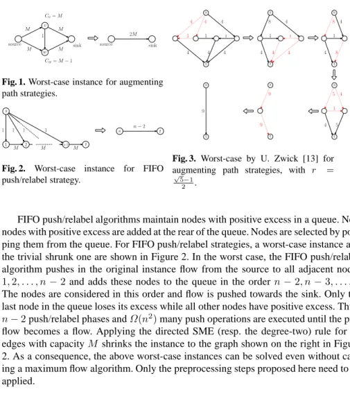
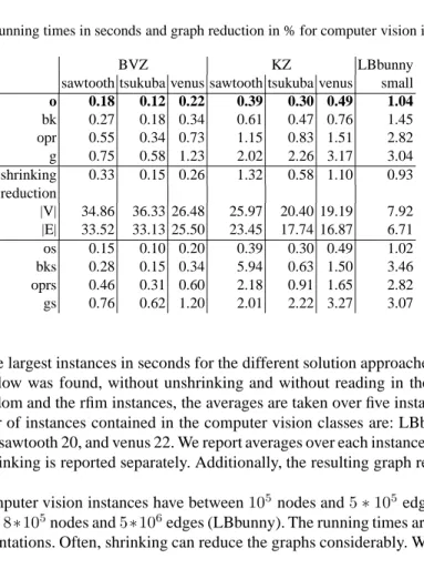
only consist of source and sink node. Figures 1 and 3 show worst-case instances for augmenting path algorithms (cf. [2]).2M augmenting steps are needed for solving the instance in Figure 1. Using non-rational capacities as in Figure 3 from [13] can even prohibit augmenting path strategies to terminate. The instance from Figure 1 can be transformed into an equivalent one by shrinking the cycle of length three that contains the source. The result is shown on the right in Figure 1. Applying shrinking operations on the dotted (red) cycles shown in Figure 3 and capacity normalizations on the dotted (red) edges, we arrive again at a trivial equivalent case.
M
M M
M
1
source sink source sink
2M Cv=M
Cw=M−1
v
w
Fig. 1. Worst-case instance for augmenting path strategies. s t M M M 1 1 1 1 n−2 1 2 n-2 s t
Fig. 2. Worst-case instance for FIFO push/relabel strategy. 4 4 4 4 4 4 1 1 r s t 4 4 4 4 8 1 r s t 4 4 8 8 1 s t 9 s t 9 9 s t 4 4 5 5 1 s t
Fig. 3. Worst-case by U. Zwick [13] for augmenting path strategies, with r =
√ 5−1
2 .
FIFO push/relabel algorithms maintain nodes with positive excess in a queue. New nodes with positive excess are added at the rear of the queue. Nodes are selected by pop-ping them from the queue. For FIFO push/relabel strategies, a worst-case instance and the trivial shrunk one are shown in Figure 2. In the worst case, the FIFO push/relabel algorithm pushes in the original instance flow from the source to all adjacent nodes 1,2, . . . , n−2 and adds these nodes to the queue in the ordern−2, n−3, . . . ,1. The nodes are considered in this order and flow is pushed towards the sink. Only the last node in the queue loses its excess while all other nodes have positive excess. Thus,
n−2push/relabel phases andΩ(n2)many push operations are executed until the pre-flow becomes a pre-flow. Applying the directed SME (resp. the degree-two) rule for all edges with capacityM shrinks the instance to the graph shown on the right in Figure 2. As a consequence, the above worst-case instances can be solved even without call-ing a maximum flow algorithm. Only the preprocesscall-ing steps proposed here need to be applied.
3
Hybrid Maximum Flow Algorithm
In this section, we propose a hybrid algorithm that in a preprocessing step shrinks node sets according to the rules presented in Section 2. Subsequently, we start increasing
flow through the network in a greedy fashion, using only short augmenting paths whose lengths do not exceed a certain threshold. This step either finds a maximum flow or a (good) initial flow. In the latter, the flow is increased further to an optimal one by some known maximum flow algorithm. Depending on the problem structure, we either use a lowest push/relabel approach or an augmenting path strategy. The performance of different maximum flow algorithms strongly depends on the problem structure. For example, while some approach may perform well on sparse graphs, it might take long on dense instances, or vice versa. As it is known [6] that the ‘double tree’ augmenting path strategy by Boykov and Kolmogorov [3] is especially fast on sparse instances, we use it in the latter case. For dense instances, a lowest push/relabel approach performs considerably better than the ‘double tree’ procedure and is preferable in this case. We thus exploit the algorithmic advantages of the different methods. After having solved the problem to optimality, all shrunk nodes have to be expanded. The optimum flow has to be rerouted accordingly. The hybrid algorithm is outlined in Algorithm 1. The general idea in the depth-restricted flow augmentation phase is to label the nodes de-pending on the labels of their local neighborhood. This yields a rough classification of the node set with regard to their distance fromsandt. The labeling then controls a depth-restricted flow augmenting step which is performed until no augmenting path between source and sink is found. As it would take too long to determine node labels exactly, we only determine whether a node is ‘near to’ the source and/or near to the sink or not. Intuitively, greedy augmenting paths between nodes that are far away from the source and the sink are allowed to be longer than those between nodes that are near to the source and the sink. In the following, we explain the details of this greedy step.
Algorithm 1: hybrid maximum flow algorithm 1: apply shrinking rules
2: label nodes 3: repeat
4: depth-restricted flow augmentation 5: update node labels afterraugmentations
6: until no augmenting path with prescribed length betweensandtis found 7: switch to ‘double tree’ or ‘push/relabel’ strategy
8: undo shrinking steps, reroute the flow locally
We assign node labelsS, T, ST, N that indicate whether a node is adjacent only tos, only tot, to bothsandt, or whether it is neither adjacent tosnor tot, respectively. We subsequently refine the label of each node depending on the inital labels of its adjacent nodes. The label refinement for node v is independent of its own initial label. Supposevis adjacent only to nodes labeled byT(resp.ST,S). Then the refined label is OT (OT,OS, respectively). Otherwise, if at least one but not all neighbors ofvare labeled byT orST, then the refined label is set toN T. Ifv does not have a neighbor labeled byT orSTbut at least one neighbor with labelS, thenvreceives the refined labelN S. In the remaining cases, the refined label is set toON. The labeling is determined by a breath-first search starting at the source and uses the initial labels
S, T, ST, N only. With the labeling at hand we search for augmenting paths from nodes with initial labelS. We restrict the length of those paths depending on the refined node label. These paths are short and can be checked fast. The labels may be updated after some depth-restricted augmentations and the augmenting search may be repeated. In our experiments we found that afterr= 5augmentations, a label update should be performed.
The definition of the path lengths depends on the problem. Setting the thresholds to a large value increases the running time without yielding considerably better flows. Set-ting them to a very small threshold keeps the running time low but only yields flows with very small values. In our tests, we found good performance for the following depths: 1 (OT), 3 (N T), 7 (OS), andmin{|¯δ+20(s)|,14} (ON). For nodes with refined label
ON we incorporate¯δ+(s)the degree of the source in the residual graph. This should prohibit the usage of long paths if the source is only sparsely connected in the residual graph. Our computational results in the next section indicate that this hybrid algorithm works well on the classes of instances occurring in physics and in computer vision.
4
Computational Results
Among the many applications for maximum flows in graphs, we focus here on applica-tions in computer vision and in theoretical physics. Although these applicaapplica-tions are in different areas, the typical instances share a similar structure. In the random-field Ising model (RFIM) from theoretical physics, the so-called base graph is a two- or three-dimensional grid graph in which all edges have the same capacity. Furthermore, each node in the grid is either connected to the additional nodesor totwith equal probability. The latter edges can have different capacities. Networks with a similar graph structure but different capacity choices also occur in image segmentation or image restoration applications in computer vision.
More specifically, our experiments focus on the following different instance types: (vision) directed computer vision instances [1] as reported in [3,6] with integral capacities
(rfim) (directed and undirected) RFIM instances as for example proposed in [8].
We used the value4as capacity for the edges in the base graph. The capacity of the edges containing the source or the sink take integer values that depend on some parameter∆, where larger value of∆ yields larger capacities, see [8]. We tested
∆= 1,4,8and used varying grid sizes up to15002in 2D and up to2003in 3D.
(random) (directed and undirected) sparse random instances generated with the graph generator ‘rudy’ [12] as
rudy -rnd_graph 500000 D S -random 1 100 SwithD = 1and2 the density parameter, seedS, and capacities in the range[1,100]. We considered different variants in which we varied the probability of nodes being connected to the source (resp. the sink). We call the variant in which all nodes of the base graph are connected tosortwith equal probability 100% connected. According to the probabilityP with which the nodes are connected to either source or sink, we use the nameP%connected withP ∈ {10, 20, 30, 40, 50, 100}. The capacity for the edges from source (resp. sink) to the nodes in the basis graph was drawn from an interval that was10times larger than the capacities of edges in the basis graph.
Due to the specific structure, many cycles of length three are present in all instance classes which makes shrinking possible. We evaluate the following algorithms and im-plementations:
(g) highest push/relabel implementation by Goldberg [7] for directed graphs with inte-ger capacities
(j) ‘mincut-lib’ by Jünger et al. [9] with a fast implementation of a ‘highest push/relabel’ algorithm for undirected graphs
(bk) ‘double tree’ implementation by Boykov and Kolmogorov, specialized for com-puter vision instances [3],
(o) hybrid method with the ‘double tree’ implementation by Boykov and Kolmogorov [3] in the second step
(pr) hybrid method with a lowest label push/relabel implementation in the second step. In the tables the abbreviations ((g), (j), (bk), (o), (pr)) are suffixed by ‘s’ if used on the shrunk graph. All computations were carried out on IntelR Xeon cCPU E5410
2.33GHz (16GB RAM) (running under Debian Linux 5.0). Implementations (o) and (pr) are based on the graph library OGDF [10]. In Tables 1-3 we report average running
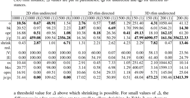
Table 1. Running times in seconds and graph reduction in % for computer vision instances.
BVZ KZ LBbunny
sawtooth tsukuba venus sawtooth tsukuba venus small o 0.18 0.12 0.22 0.39 0.30 0.49 1.04 bk 0.27 0.18 0.34 0.61 0.47 0.76 1.45 opr 0.55 0.34 0.73 1.15 0.83 1.51 2.82 g 0.75 0.58 1.23 2.02 2.26 3.17 3.04 shrinking 0.33 0.15 0.26 1.32 0.58 1.10 0.93 reduction |V| 34.86 36.33 26.48 25.97 20.40 19.19 7.92 |E| 33.52 33.13 25.50 23.45 17.74 16.87 6.71 os 0.15 0.10 0.20 0.39 0.30 0.49 1.02 bks 0.28 0.15 0.34 5.94 0.63 1.50 3.46 oprs 0.46 0.31 0.60 2.18 0.91 1.65 2.82 gs 0.76 0.62 1.20 2.01 2.22 3.27 3.07
times for the largest instances in seconds for the different solution approaches until the maximum flow was found, without unshrinking and without reading in the instance. For the random and the rfim instances, the averages are taken over five instances each. The number of instances contained in the computer vision classes are: LBbunny one, tsukuba 16, sawtooth 20, and venus 22. We report averages over each instance class. The time for shrinking is reported separately. Additionally, the resulting graph reduction is given in %.
The computer vision instances have between105nodes and5∗105edges
(BVZt-sukuba) and8∗105nodes and5∗106edges (LBbunny). The running times are small for
time, the sizes are reduced by about7%to35%. However, the programs often cannot profit from the reduced graph sizes as computing an optimum solution on the shrunk graph takes almost the same running time as on the original one. Our new hybrid imple-mentation without shrinking (o) is however considerably faster than the impleimple-mentation (g). Moreover, it is always the fastest method. It can even improve over the pure ‘dou-ble tree’ strategy (bk). This is remarka‘dou-ble as (bk) is the state-of-the-art maximum-flow implementation for instances from computer vision. For the 2D rfim instances, there is
Table 2. Running times in seconds and graph reduction in % for two- (2D) and three-dimensional (3D) rfim instance,∆values are put in parentheses, (j) for undirected and (g) for directed
in-stances.
2D rfim undirected 2D rfim directed 3D rfim undirected
1000 (1) 1000 (8) 1500 (1) 1500 (8) 1000 (1) 1000 (8) 1500 (1) 1500 (8) 150 (1) 150 (8) 200 (1) 200 (8) o 10.56 0.67 48.91 1.54 2.76 0.57 7.05 1.29 251.40 4.31 1050.44 41.12 bk 20.52 0.97 98.23 2.23 2.87 0.80 6.69 1.70 399.86 6.01 1546.21 14.30 opr 16.88 0.51 69.56 1.08 10.38 0.18 26.36 0.41 49.13 18.10 162.15 61.20 j/g 31.40 459.08 109.54 2356.28 16.36 0.58 50.29 1.34 47.99 6090.57 161.56 35622.33 shrink 0.43 2.87 1.01 6.71 1.31 2.21 2.62 4.23 2.29 7.82 0.47 13.46 red. |V| 0.00 100.00 0.00 100.00 0.10 60.00 0.07 60.00 0.00 58.13 0.00 23.56 |E| 0.00 100.00 0.00 100.00 0.06 54.19 0.04 54.19 0.00 61.40 0.00 24.79 os 10.44 0.00 49.00 0.01 2.91 0.45 7.33 1.05 251.62 2.10 1044.82 10.14 bks 20.77 0.00 98.00 0.00 3.14 0.58 6.98 1.29 400.07 3.16 1599.13 14.14 oprs 16.91 0.00 69.51 0.00 10.66 0.54 29.33 1.18 49.09 5.71 145.04 25.04 js/gs 31.44 0.00 109.62 0.00 17.02 0.22 50.89 0.51 48.04 673.23 190.46 13413.39
a threshold value for∆above which shrinking is possible. For small values of∆, the differences in edge capacities are too small to allow shrinking. In Table 2, we show re-sults for the largest graphs, where capacity choices are below and above the threshold. Above the threshold, shrinking can be performed fast and yields a drastic graph reduc-tion, sometimes even by 100%. It however has almost no effect on the running time except when using the implementation [9]. The latter needs much longer on the original graph, while the graph can be shrunk to a trivial equivalent instance in a few seconds. When compared to undirected instances, the shrinking steps need longer for directed graphs. For dense directed graphs, shrinking may be counterproductive as can be seen in Table 3. Although the graph size is drastically reduced, the total running times in-creases. On those instances, each augmentation step takes longer while the number of augmentations remains similar. Let us consider the implementations without shrinking. The hybrid variants perform comparable or better than the traditional algorithms on two-dimensional instances. For undirected graphs, the running time can considerably be reduced in the highest push/relabel approach when first the depth-restricted flow augmentation is applied. The situation is similar for 3D rfim instances. For directed graphs, the highest push/relabel (g) implementation is slightly faster on average than the hybrid versions. Due to memory limitations, directed instances of size2003could
Table 3. Running times in seconds and graph reduction in % for random instances. (k = 103
,
M = 106, graph size of the random base graph whithout edges to source and sink, (j) for undi-rected and (g) for diundi-rected instances.)
random undirected directed
rfim 50% connected 100% connected 50% connected 100% connected 500k (4.5M) 500k (9M) 500k (4.5M) 500k (9M) 500k (4.5M) 500k (9M) 500k (4.5M) 500k (9M) o 47.46 160.58 11.02 132.95 3.65 15.14 3.06 9.92 bk 75.62 233.49 15.39 246.72 4.42 18.72 3.76 14.13 opr 14.59 9.89 35.92 17.36 10.24 46.75 6.54 36.82 j/g 13.12 10.05 77.17 19.71 3.03 8.92 2.53 7.19 shrink 1.24 0.77 3.61 3.03 10.76 12.98 22.12 37.97 red. |V| 9.02 0.03 20.91 0.05 28.86 16.01 56.57 41.45 |E| 7.06 0.01 23.95 0.03 29.67 18.11 60.17 54.37 os 39.92 159.98 7.43 132.82 2595.02 1289.10 2694.99 2014.12 bks 63.05 231.77 10.66 243.05 3674.14 2669.79 3476.53 5725.78 oprs 10.50 9.72 25.81 17.37 1889.02 1170.80 1783.09 1703.39 js/gs 11.89 9.91 54.03 20.46 2.28 7.76 0.98 4.02
For the physics instances, implementation (o) needs the same number of augmenting steps as (bk), most of them take place in the greedy step. This is also true for the directed random instances. On the other hand, on the undirected random instances (o) needs considerably less augmentation steps than (bk).
Although the preprocessing steps introduced above have mainly been designed for the applications mentioned above, it is interesting to evaluate them on random instances. As can be expected, shrinking has no effect for random instances in which less than 50%of the nodes in the base graph are adjacent to source or sink. The graph size is then reduced by at most 6%. This can be understood as not many small cycles are present that contain edges of large capacity. The corresponding running times show the same characteristics as those given in Table 3 and are therefore skipped. We note it is advantageous to apply our algorithm on undirected graphs in which the nodes in the base graph are highly connected to the source and the sink. Otherwise, traditional methods like (g) are preferable. This is especially true for directed graphs.
As a summary, our hybrid algorithm without shrinking reduces the running time on undirected random instances that are highly connected to source and sink, furthermore on vision and rfim instances. There, it even improves the method (bk) which is the currently fastest available program for sparse graphs. The running time of the hybrid implementation with the ‘double tree’ strategy (o) is at least comparable or faster than (bk).
5
Conclusion
In this work, we proposed preprocessing routines for maximum flow algorithms. We showed that the input size can be reduced by shrinking node subsets while preserving
an optimal solution. Moreover, well-known worst-case instances for different maximum flow algorithms can be transformed into trivial equivalent instances.
Subsequently, we presented a depth-restricted augmenting path algorithm that yields very fast a good initial flow. In combination with known solution strategies, the running times of traditional maximum flow algorithms are considerably reduced on relevant instances from physics and computer vision. Taking the special graph structure into account, shrinking can remarkably reduce the graph sizes and also the running time of highest push/relabel algorithms on undirected graphs. Nevertheless, shrinking has to be applied with care: For directed graphs, the running time can increase as each augmentation step takes longer. For instances from theoretical physics and computer vision, the fastest method uses augmenting path strategies without shrinking but with the new depth-restricted augmentation step as proposed here. For directed instances, the implementation from [7] is the fastest one. It however can only be used for integral capacities.
References
1. Computer vision instances: http://vision.csd.uwo.ca/maxflow-data.
2. R. K. Ahuja, T. L. Magnanti, and J. B. Orlin. Network Flows: Theory, Algorithms, and
Applications. Prentice Hall Inc., 1993.
3. Y. Boykov and V. Kolmogorov. An Experimental Comparison of Min-Cut/Max-Flow Al-gorithms for Energy Minimization in Vision. IEEE Trans. Pattern Anal. Mach. Intell.,
26(9):1124–1137, 2004.
4. E. A. Dinic. An algorithm for the solution of the problem of maximal flow in a network with power estimation. Dokl. Akad. Nauk SSSR, 194:754–757, 1970.
5. L. R. Ford, Jr. and D. R. Fulkerson. Maximal flow through a network. Canad. J. Math., 8:399–404, 1956.
6. A. V. Goldberg. The partial augment-relabel algorithm for the maximum flow problem. In
ESA ’08: Proceedings of the 16th annual European symposium on Algorithms, pages 466–
477, Berlin, Heidelberg, 2008. Springer-Verlag.
7. A. V. Goldberg and R. E. Tarjan. A new approach to the maximum-flow problem. J. Assoc.
Comput. Mach., 35(4):921–940, 1988.
8. A. H. Hartmann and H. Rieger. Optimization Algorithms in Physics. Wiley-VCH Verlag GmbH & Co. KGaA, 2003.
9. M. Jünger, G. Rinaldi, and S. Thienel. Practical performance of efficient minimum cut algo-rithms. Algorithmica, 26:172–195, 2000.
10. OGDF. Open Graph Drawing Framework. http://www.ogdf.net, 2007.
11. M. Padberg and G. Rinaldi. An efficient algorithm for the minimum capacity cut problem.
Math. Programming, 47(1, (Ser. A)):19–36, 1990.
12. G. Rinaldi. rudy – A rudimentary graph generator: https://www-user.tu-chemnitz.de/~helmberg/rudy.tar.gz, 1998.
13. U. Zwick. The smallest networks on which the Ford-Fulkerson maximum flow procedure may fail to terminate. Theoretical Computer Science, 148(1):165 – 170, 1995.
Appendix
In this section, we show the proofs for shrinking certain node sets as presented in Sec-tion 2.
Proof (Lemma 1). Let w.l.o.g.Cv = max{Cv, Cw, cqv+cqw}. Note that the value of a feasible flow through supernodevw using edges formerly incident tov (tow,q, resp.) is bounded byCv (resp.Cw,cqv +cqw). SupposeCw units of flow (which is the maximum amount of flow throughvwusing edges formerly incident tow) should be rerouted fromv tow. Routecvw units directly fromv tow. The remaining units
Cw−cvwcan be rerouted overq, because the shrinking condition
cqv+cvw≥max{Cv, Cw}=Cv
was satisfied. Therefore, it iscqv ≥Cw−cvw. The same is true for edge(qw)so that we havecqw ≥Cw−cvw.
Using similar arguments,cqv+cqw units of flow (which is the maximum amount of flow throughvw using edge(q, vw)) can be rerouted toq. First we routecqv units over(q, v).cqw ≤Cv−cqvunits can be routed to nodewusing edge(v, w)ascvw≥
Cv−cqv≥cqw.⊓⊔
Proof (Lemma 2). Assume the SME rules have already been applied such that the SME condition is not satisfied for any edgee∈EZ. The proof is analogous to that of Lemma 1: We show that any feasible flow through the supernode can be rerouted locally in the subgraphHq,Z. We need to consider different cases. Suppose there exists a node
z ∈ Z that is in Hq,Z only adjacent toq. As (1) is satisfied forW = {z} ⊂ Z, it follows thatcqz ≥ Cz−cqz. Let f denote the amount of flow that passes through the supernode using edges formerly incident tozi ∈ Z. Thus, we have to reroutef units of flow viaqtoz. Consider any nodezi ∈ Z \ {z} withCzi =
P
g∈∆(zi)cg
where∆(zi) = {(zi, w)| w 6= q, w 6∈ Z}. LetCz = min{Cz, Czi}be the limiting
capacity, i.e. the maximum amount of flow that can pass the supernode in the shrunk graph through edges formerly incident toz orzi. If nodezi is only adjacent toqin the subgraphHq,Z, thenCz flow units can be routed toq and then toz as it holds
cqzi ≥Czi−cqzi≥Cz−cqzi. If there exists an edge(zi, zj)withzj∈ZinEZ, then
the nodesq, zi, zjform a cycle of length three. In this case, we reroutecqzi =Cz−c(zi: Z\ {zi})flow units toqvia(q, zi)and further tozvia(q, z). The remaining amount of flowCz−c(zi:Z\ {zi})≤czizjis routed tozj. Supposeziandzjare part of only
one such cycle. ConsiderW ={zi, zj} ⊂Zthenc(W :Z\W) = 0andCW−c(W :
q) ≤ c(W : q). We already sentcziq units flow fromzi toqover edge(zi, q), thus Cv−czq+Czj −c(W : q) ≤ c(zj : q). Therefore we can reroute the remaining
amount of flow toqand then toz. If there exists an edge(zj, zl)withzi 6=zl ∈Zin
EZ,nodezj is part of another cycle of length three and the argumentation is applied recursively. This is also done ifziis part of several cycles of length three. If there exists an edge(z, zj)withzj ∈ZinEZ, thenzis not only adjacent toqinHq,Z and similar arguments are used to first route every possible flow toqand then toz. The remaining flow units can be sent over the cut-edges betweenzandZ\ {z}in the same way as
s vw csv+csw csv cvw csw v w s ? ch cl ch cl h l l h
Fig. 4. Rerouting flow in the directed case.
Proof (Lemma 3). The only interesting case is the one displayed in Figure 4 as other cases directly follow from it. Suppose there is flow fromsandlpassing the supernode to nodehin the shrunk graph. This flow cannot be rerouted locally in the cycle as the direction of the edge forbids to send flow from nodewto eithersorv. We however can reroute the amount of incoming flowfat nodewback to the sources. This is possible as the considered flow is feasible. Moreover, thef units of flow can be sent via edge
sv. This is possible because it holdscsv ≥Pg∈δ+(v)cg−cvw−cwv. For the specific example shown in Figure5, we havecsv≥ch. For supernodexywe do not need to use any global rerouting. The maximum amount of flow that reachesthas valuecxt+cyt. It is not difficult to see that this amount of flow can be rerouted locally within the directed
cycle. ⊓⊔ s vw csv+csw csv cvw csw v w s ch cl ch cl h l l h
sent flow back to source