A hardware reconstruction system for real-time magnetic resonance imaging via 2D FFT or filtered backprojection

A hardware reconstruction system for real-time magnetic

resonance imaging via 2D FFT or filtered backprojection

Authors Ehsani, Ali Reza,

1963-Publisher The University of Arizona.

Rights Copyright © is held by the author. Digital access to this material is made possible by the University Libraries, University of Arizona. Further transmission, reproduction or presentation (such as public display or performance) of protected items is prohibited except with permission of the author.

Download date 22/01/2021 01:00:56

This manuscript has been reproduced from the microfilm master. UMI films the text directly fi'om the original or copy submitted. Thus, some thesis and dissertation copies are in typewriter

&ce,

The quality of this reproduction is dependent upon the quality of the copy submitted. Broken or indistinct print, colored or poor quality illustrations and photographs, print bleedthrough, substandard margins, and improper alignment can adversely affect reproduction.

In the unlikely event that the author did not send UMI a complete manuscript and there are missing pages, these be noted. Also, if unauthorized copyright material had to be removed, a note will indicate the deletion.

Oversize materials (e.g., maps, drawings, charts) are reproduced by sectioning the original, beginning at the upper left-hand comer and continuing fi-om left to right in equal sections with small overiaps. Each original is also photographed in one exposure and is included in reduced form at the back of the book.

Photographs included in the original manuscript have been reproduced xerographically in this copy. Ifigher quality

6" x

UMI

A Bell & Howell Infonnation Company

300 North Zed) Road, Ann Aibor MI 48106-1346 USA 313/761-4700 800/521-0600

RESONANCE IMAGING VIA 2D FFT OR FILTERED BACKPROJECTION

by

Ali Reza Ehsani

Copyright © Ali Reza Ehsani 1996

A Dissertation Submitted to the Faculty of the

DEPARTMENT OF ELECTRICAL AND COMPUTER ENGINEERING

In Partial Fulfillment of the Requirements For the Degree of

DOCTOR OF PHILOSOPHY

In the Graduate College

THE UNIVERSITY OF ARIZONA

DMI Number: 9720645

UMI Microform 9720645

Copyright 1997, by UMI Company. All rights reserved. This microform edition is protected against unauthorized

copying under Title 17, United States Code.

UMI

THE UNIVERSITY OF ARIZONA ® GRADUATE COLLEGE

As members of the Final Examination Committee, we certify that we have read the dissertation prepared by All Reza Ehsani

entitled A HARDWARE RECONSTRaCTION SYSTEM FOR REAL-TIME MAGNETIC RESONANCE IMAGING VIA 2D FFT OR

FILTERED BACKPROJECTION

and recommend that it be accepted as fulfilling the dissertation requirement for the Degree of Doctor of Philosophy

Date

Date / ' Date

yA

'f

Date

Final approval and acceptance of this dissertation is contingent upon the candidate's submission of the final copy of the dissertation to the Graduate College.

I hereby certify that I have read this dissertation prepared under my direction and recommend that it be accepted as fulfilling the dissertation requirement^

ssertation Director

3

STATEMENT BY AUTHOR

This dissertation has been submitted in partial fulfillment of requirements for an advanced degree at The University of Arizona and is deposited in the University Library to be made available to borrowers under rules of the Library.

Brief quotations from this dissertation are allowable without special permission, provided that accurate acknowledgment of source is made. Requests for permission for extended quotation from or reproduction of this manuscript in whole or in part may be granted by the copyright holder.

ACKNOWLEDGMENTS

I would like to thank Professor Arthur F. Gmitro for his guidance, supervision, enthusiasm and most of all his friendship. His willingness to spend so many hours in the lab and working on this project was greatly appreciated. The extraordinary working atmosphere he created, made the completion of this project much easier. I am tmly fortunate to have worked on such an interesting project with such an extremely knowledgeable individual.

I also wish to thank my major advisor. Professor John A. Reagan for his great support throughout my graduate studies. The experiences that I obtained from my master's thesis under his supervision, were very beneficial in fulfilment of my Ph.D. project.

I would also like to extend my gratitude to Dr. Ted Trouard, Constantin Job (Don), and Dr. Maria Altbach for their assistance in running the Bruker Biospec as well as their helpful suggestions in the development of the real-time system. Also, many thanks are due to former graduate student Troy Berchem who operated the Bruker Biospec and helped with the debugging and wire-wrapping of the circuit boards.

To my wife,

my family

TABLE OF CONTENTS

2. INTRODUCTION TO MAGNETIC RESONANCE IMAGING 23

2.1 BASIC PRINCIPLES OF NMR 23

2.1.1 The Bloch Equations 26

2.1.2 Relaxation 33

2.1.3 Free Induction Decay 36

2.2 BASIC PRINCIPLES OF MRI 37

2.2.1 Slice Selection 38

2.2.2 Spatial Encoding 41

2.3 THE NMR SIGNAL DETECTION SYSTEM 46

2.3.1 RF Coil 46

2.3.2 Signal Processing 48

3. MRI ACQUISITION AND RECONSTRUCTION METHODS 50

3.1 MULTIPLE-SHOT MR ACQUISITION METHODS 51

3.1.1 Spin-Echo 51

3.1.2 Gradient-Echo 54

3.2 SINGLE-SHOT MR ACQUISITION METHODS 56

3.2.1 Single-Shot Data Acquisition Concerns 59

3.3 MRI RECONSTRUCTION METHODS 61

3.3.1 2D Fourier Imaging 61

3.3.2 Projection Imaging 62

7

4.1 GENERAL INFORMATION 69

4.1.1 The A41102 FFT Chip 70

4.2 ADC Board 75

4.3 INTERFACE MEMORY (IM) BOARD 78

4.4 DISPLAY PROCESSOR (DP) BOARD 83

5. THE 2D FFT HARDWARE RECONSTRUCTION SYSTEM 86

5.1 COLUMN/ROW DECOMPOSITION 88

5.2 THE 2D FFT HARDWARE 93

6. THE FILTERED BACKPROJECTION HARDWARE RECONSTRUCTION 101

6.1 DISCRETE FILTERED BACKPROJECTION ALGORITHM 103

6.2 THE PROJECTION FILTER HARDWARE 107

6.3 THE BACKPROJECTION HARDWARE 113

7. RESULTS 123

7.1 RESULTS FROM THE 2D FFT HARDWARE 123

7.1.1 Gradient-Echo Results 125

7.1.2 Echo-Planar Results 131

7.2 RESULTS FROM THE FILTERED BACKPROJECTION HARDWARE ... 135

7.2.1 Gradient-Echo (Radial-Scan) Results 136

7.2.2 Echo-Planar (Spiral-Scan) Results 137

8. CONCLUSIONS AND FUTURE DIRECTION 140

8.1 CONCLUSIONS 140

8.2 FUTURE DIRECTION AND IMPROVEMENTS 142

8.2.1 K-space Data Interpolation 142

8.2.2 Real-Time Digital Data Storage 143

8.2.3 128 X 128 Filtered Backprojection Reconstruction System 144

8.2.4 Image Contrast and Brightness Adjustments 146

Figure 1.1 Interface between the real-time MRI hardware reconstruction system and

the MRI machine 18

Figure 2.1 A single nuclei with a magnetic moment, and an angular momentum, I, precessing about the static field, Bq, at the Larmor frequency, to 24

Figure 2.2 The effect of RF pulse on spin magnetization, (a) net magnetization in equilibrium lies along the static field, (b) application of the RF filed causes a rotation of the net magnetization towards the transverse plane 25

Figure 2.3 Formation of 3^,^ in the rotating frame, (a) is not in the x-y plane when co*ci)o, (b) is along the x'-axis when a)=(0o 30

Figure 2.4 The effect of RF pulses with different flip angles on the net magnetization

in the rotating firame 32

Figure 2.5 T, and T, relaxations are simultaneous processes with T2 being much

shorter than T, 35

Figure 2.6 Application of RF pulses at different frequencies results in excitation of different slices along and perpendicular to the z-axis 39

Figure 2.7 Slice selection procedure, (a) Graph of o) vs z, shows the relationship between the carrier frequency of the RF pulse, with the location of excited slice, (b) Application of a sine shaped RF pulse with the slice gradient, excites a nearly uniform frequency distribution (slice profile) 40

Figure 2.8 Scanning the k-space. (a) The pulse sequence for a typical gradient-echo sequence, (b) The corresponding trajectory path taken through the k-space, from S) on the z-axis (center of k-space), pre-positioned to and a

horizontal read-out from @ to ® with a maximum echo at point (D 43

Figure 2.9 Gradient-echo pulse sequence for radial-scan, (a) The gradient-echo pulse sequence for a typical radial-scan in k-space. (b) The corresponding trajectory path taken through the k-space, from ® on the origin (center of k-space), pre-positioned to and a radial read-out from @ to @ with a

9

Figure 2.10 The RF coil receiver and the quadrature demodulation circuit 47

Figure 3.1 Spin-echo pulse sequence for raster-scan 52

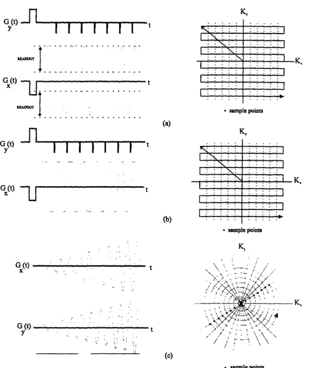
Figure 3.2 Single-shot acquisition methods and the location of sample points in k-space. (a) Slipped echo-planar imaging, (b) Modified blipped echo-planar imaging, (c) Spiral-scan echo-planar imaging 58

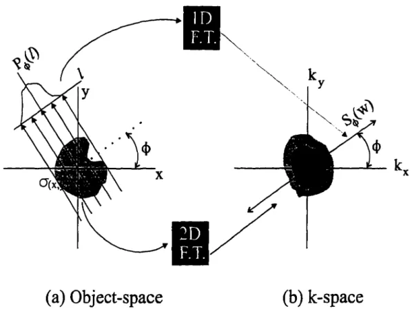
Figure 3.3 The Fourier slice theorem, (a) The function P^(/) is the projection of a(x,y) at angle (J), (b) The corresponding radial line in k-space is the

Fourier transform of the projection 65

Figure 4.1 Block Diagram of the real-time reconstruction system. There are three circuit boards common in both reconstruction methods: the analog-to-digital convertor (ADC) board, the interface memory (IM) board, and the

display processor (DP) board 68

Figure 4.2 Block diagram of the A41102 FFT chip 71

Figure 4.3 Timing diagram oftheA41102 chip 73

Figure 4.4 Block diagram of the ADC board 76

Figure 4.5 Timing diagram for the input and output of the ADC board 77

Figure 4.6 Block diagram of the Interface Memory (IM) board 79

Figure 4.7 Timing diagram of the IM board 80

Figure 4.8 Block Diagram of the Display Processor (DP) Board 84

Figure 5.1 The 2D FFT reconstruction board and the ribbon cable connections 87

Figure 5.2 Block diagram of the Fourier Processor (FP) board 88

Figure 5.3 The column/row decomposition method, (a) colunm selection in the k-space, (b) Fourier transform of the columns are bit-reversed, (c) row selection and reordering of data for bit-reversal correction, (d) the 2D inverse fast Fourier transformed reconstructed image 90

Figure 5.4 Figure 5.5 Figure 5.6 Figure 6.1 Figure 6.2 Figure 6.3 Figure 6.4 Figure 6.5 Figure 6.6 Figure 6.7 Figure 6.8 Figure 7.1 Figure 7.2 Figure 7.3 Figure 7.4

(a) The effect of checkerboarding on image reconstruction, (a) The center of the reconstructed image does not fall at the center of displayed image, (b) multiplying the k-space data by a 2D "checkerboard" pattern to result

in a shift in the object space. 92

Example of an 8 x 8 checkerboard pattern 93

Timing diagram of the FP board 94

The filtered backprojection reconstruction boards and the ribbon cable

connections 102

The discrete filter H[w] 104

The backprojection method 106

Block diagram of the Projection Filter (PF) board 108

Timing diagram of the PF board 109

Block diagram of the Backprojection (BP) board 114

Sequence of events for the different functions on the BP board 114

Timing diagram of the BP board 115

The 2D FFT hardware can be tested by writing a test pattern to the interface memory of the IM board. The 256 x 256 reconstruction of a 2D rect function results in a (magnitude) 2D sine function. The

reconstruction is performed in 32.8 ms 125

A plastic phantom with an X pattern plastic-insert was used in some of the experiments. The phantom is filled with water 127

A gradient-echo pulse sequence (raster-scan) is utilized with the 2D FFT hardware system to reconstruct the image of the plastic phantom. The 256

X 128 k-space is scanned in 2 seconds 128

Image of a rat moved through the bore of the RF coil using a gradient-echo pulse sequence (Snapshot) at 4 frames/sec. (a) The rat's heart is captured in one still frame, (b) The rat's head is shown in another still frame.... 130

II Figure 7.5 Figure 7.6 Figure 7.7 Figure 7.8 Figure 7.9 Figure 8.1

Block diagram of the real-time 2D FFT reconstruction system with the digital interface (DI) board replacing the ADC board 132

Results from the 2D FFT hardware reconstruction system interfaced to a clinical MRI system with EPI capabilities. A sequence of 12 unages from a human subject moving through the magnet are shown from time t=0 to

t=l 1 seconds 134

An image reconstructed by the filtered backprojection hardware. The filtered backprojection hardware can be tested by writing a test pattern to the interface memory of the IM board. The 64 x 64 reconstruction of a 2D sine function results in a 2D rect function shown 135

Phantom image obtained with a gradient-echo pulse sequence (radial-scan). The k-space is scanned at a rate of I frame/sec are reconstructed

with the filtered backprojection system 137

Phantom image obtained with a SEPI pulse sequence. The k-space data are scanned at a rate of 25 frames/sec and are reconstructed with the

filtered backprojection system 139

Example of a 128 x 128 backprojection circuit using a parallel adder network. Utilizing this scheme, a reconstruction rate of 38 frames/sec can

LIST OF TABLES

Table 3.1 Contrast enhancement in spin-echo by manipulation of TR and TE 53

Table 4.1 Cable connections to the real-time system 69

ABSTRACT

13

A "real-time" hardware reconstruction system for Magnetic Resonance Imaging (MRI)

has been designed, constructed, and demonstrated. Here, "real-time" corresponds to frame

rates of 30 or more per second (i.e., video rate). The system is capable of reconstructing

images via either the 2D FFT algorithm or the filtered backprojection algorithm. The 2D FFT

hardware reconstructs 256 x 256 images from complex-valued data (on a rectilinear grid) at

a rate of 30 frames/sec while the filtered backprojection hardware is capable of

reconstructing 64 x 64 images from complex-valued data (on a polar grid) at a rate of 37

frames/sec. Real-time MRI may be achieved by interfacing the reconstruction system to MR

scanners with ultra-fast acquisition capabilities, such as echo-planar imaging (EPI) for

rectilinear data or spiral-scan for polar data.

The reconstruction system consists of a number of circuit boards plugged into the bus

of a personal computer (PC). The circuit boards are configured by the PC, and thereafter,

communicate with each other through ribbon cables independent of the PC operation. Three

of the circuit boards are common in both reconstruction methods. They are an

analog-to-digital converter board (ADC), an interface memory board (IM), and a display processor

board (DP). In the 2D FFT method a fourth circuit board referred to as the Fourier processor

board (FP) is utilized. In the filtered backprojection method two additional circuit boards,

of the two reconstruction methods as well as design and implementation of the

digital-electronic hardware are described in this dissertation. Real-time reconstructed images by

CHAPTER 1

15

INTRODUCTION

1.1 Overview

Since 1973, when the first image of two capillary tubes was produced [1-2], the field

of Magnetic Resonance Imaging (MRI) has evolved into an indispensable medical imaging

procedure. As an imaging modality MRI has a number of significant advantages. These

include its use of non-ionizing radiation, high-resolution capabilities, high soft tissue

contrast, and capabilities of obtaining anatomic cross-sectional images in any direction. Yet

for ail of its efficacy, MRI for the most part has been a costly [8] and uncomfortable

procedure for the patient. These drawbacks are mainly due to the length of the MRI scan

times, which are long compared to physiological motion and patient tolerance. Conventional

MRI methods build images fi-om repeated excitations and data acquisition sequences. Each

image acquisition can take as long as many minutes while the patient must keep still inside

the bore of a large imaging magnet. Any motion by the subject may result in severe artifacts

in the reconstructed images [4-5]. In the case of physiological motions, such as the heart­

beat, additional provisions such as electrocardiogram (ECG) gating must be incorporated into

the imaging sequence in order to synchronize the data collection to the patient's heart-beat.

Such provisions fiirther increase the length of an imaging sequence, which results in patient

conventional MRI restricts the range of MRI applications, increases the cost of scanning by

reducing throughput, and leads to image artifacts from patient motion.

Fortunately, with recent advancements in the development of faster imaging coils (fast

gradient coils), high-speed imaging methods that allow MR scanning times as short as 30 ms

have become possible. Ultra-fast imaging methods have scan times short compared to

physiological motion, typically less than a 100 ms. Ultra-fast imaging methods [3]

effectively freeze physiological motion, such that motion related artifacts are not present in

the reconstructed images. Ultra-fast acquisition methods, such as echo-planar imaging (EPI)

[6], are increasingly being utilized in MRI applications such as dynamic cardiac imaging and

functional brain imaging. Interventional diagnostic or therapeutic procedures under MR

guidance are other emerging areas of application for ultra-fast MR acquisition methods. The

recent developments in open magnet designs will have a significant impact on the progress

of these techniques.

In general, ultra-fast acquisition methods correspond to single-shot (one-shot) imaging

procedures. In the single-shot method, one RF excitation is followed by a series of gradient

pulses, thereby collecting a complete set of MR data (Chapter 2). The collected data are then

reconstructed off-line to create the image. While the reconstruction time varies between

different computer platforms (typically from one to ten seconds), it is longer than the

dynamic processes, several frames of data must be acquired per second and reconstructed

consecutively. The raw data must be collected, digitized, reconstructed, and then displayed

at high frame rates. This puts a large burden on a non-dedicated reconstruction system,

which has no simultaneous input/output capabilities. An example of a non-dedicated

reconstruction system was recently shown by Kerr et al. [19] which employed nine

workstations to perform 128 x 128 image reconstruction at 16 frames/sec. Other approaches

using optical computers have also been attempted [9-11], but these analog methods have

been severely limited by issues of accuracy and dynamic range as well as cost. In order to

have a reconstruction system that is capable of image reconstruction and display at video

rates, a dedicated hardware reconstruction system must be implemented. The first dedicated

MRI reconstruction system was described by Wright and Riderer [7]. The image

reconstruction system provided faster update of images in so-called "fluoroscopic" mode.

That system updated images with partial Fourier data at rates up to six images per second

(maximum of 128 x 128 input or output matrix) and was the first digital-electronic

reconstruction system dedicated to providing real-time visual feedback in MRI.

In this dissertation, design of a dedicated real-time hardware reconstruction system for

MRI is discussed. The reconstruction system is a complete data acquisition, image

reconstruction and display package, housed in a personal computer. With the system

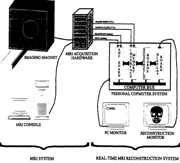
interfaced to an MRI instrument with ultra-fast acquisition capabilities (Fig. 1.1), real-time

r / MRI ACQUISITION IMAGING MAGNET/ HARDWARE

r r T r

PERSONAL COPMUTER SYSTEM

C;\MRI

MRICONSOLE

PC MONITOR RECONSTRUCTION MONITOR

MRI SYSTEM REAL-TIME MRI RECONSTRUCTION SYSTEM

Figure 1.1 Interface between the real-time MRI hardware reconstruction system and the MRI machine.

recorded for future playback. The hardware system is capable of reconstructing images via

either the 2D inverse FFT algorithm or the filtered backprojection algorithm. The 2D FFT

19

rate of 30 frames/sec. This requires a scan-pattem that produces data that lie on an

approximately rectilinear grid. The filtered backprojection hardware is configured to

reconstruct 64 x 64 images from complex-valued data of 64 lines x 64 points per Ime (polar

format) at 37 frames/sec. Data in polar format are obtained from radial line scans or are

approximated from spiral scanned data. In both of the reconstruction methods smaller

matrices of raw data may also be entered into the system (e.g., 128 x 128 scanning for 2D

FFT method or 64 lines x 32 points per line scarming for the filtered backprojection method).

These data are zero-padded by the hardware system to allow for the maximum reconstruction

size capabilities of the system. The hardware system described in this dissertation is the first

real-time MRI reconstruction system of its kind.

The hardware reconstruction system consists of a number of circuit boards plugged into

the bus (ISA bus) of a PC. The circuit boards are configiired through the ISA bus of the

computer. Once the circuit boards are programmed, the reconstruction system operates in

a pipeline fashion such that the processed data flows from one board to the next through

ribbon cables independent of the PC bus (Fig. 1.1). The reconstruction system has two

monitors, one used by the PC for initialization of the system, and the second for displaying

the reconstructed images. The interface between the MRI machine and the real-time

reconstruction system is made by a total of four connections. All of these signals originate

from the MR scanner and control the reconstruction process (Fig. 1.1). Two of the

other two lines are transistor-transistor-logic (TTL) control signals for

analog-to-digital-converter (ADC) timing and frame-reset.

The real-time reconstruction system was interfaced to a number of MRI machines The

MRI machines were programmed to generate scan patterns for rectilinear gradient-echo,

rectilinear echo-planar, radial-line gradient-echo and spiral echo-planar methods. Real-time

reconstructed images were recorded on video tapes. Selected portions of the video were

stored digitally using freeze-frame capabilities of the display processor (DP) board. These

images are presented in the results chapter (Chapter 7).

1.2 Outline

Knowledge and understanding of the MRI principles are essential in the understanding

of the real-time MRI reconstruction system presented in this dissertation. Therefore, chapter

2 is dedicated to a review of the basic NMR and MRI principles.

Chapter 3 reviews the MR image acquisition and reconstruction methods of interest.

Conventional RF pulse sequences and scaiming methods employed in this dissertation are

discussed in this chapter. The two reconstruction methods of 2D inverse FFT and filtered

backprojection utilized in the real-time hardware reconstruction system are also discussed.

In chapter 4 the general aspects of the real-time hardware reconstruction system are

21

circuit boards include the commercial data acquisition (ADC) board (PC 414, Datel Corp.),

the designed interface memory board (IM), and the commercial display processor (DP) board

(DT3851, Data Translation). The design and features of the interface memory board are

discussed in detail. Data transfer protocols between circuit boards are described. Timing

diagrams of the control signals are provided to better understand the hardware system. The

FFT chip, which is the key component of the reconstruction system and the timing signals

associated with this chip, are discussed.

Chapter 5 is dedicated to the 2D FFT hardware reconstruction design. The Fourier

processor board (FP) is described in detail. Data transfer between this board and the other

boards is also described.

Chapter 6 describes the design and implementation of the filtered backprojection

hardware system. The discrete filtered backprojection algorithm is described. The design

of the projection filter board (PF) and the backprojection board (BP) are presented. Both

circuit boards are described at the block diagram level. Timing signals of both circuits as

well as data communication between the two circuit boards and the other boards are

discussed.

Chapter 7 is the presentation of results. Images obtained from both reconstruction

interfacing the real-time system to three different MRI systems.

Chapter 8 is devoted to the conciiasions and future directions of this research. The

capabilities of the real-time hardware reconstruction system are reviewed. Possible

CHAPTER 2

23

INTRODUCTION TO MAGNETIC RESONANCE IMAGING

2.1 BASIC PRINCIPLES OF NMR

The principle of Nuclear Magnetic Resonance (NMR) is based on the interaction

between an atomic nucleus and an extemal magnetic field. The primary nucleus of interest

in MRI is the hydrogen proton ('H). This is for two reasons: (1) the high sensitivity of

hydrogen's MR signal, and (2) the high natural abundance of hydrogen in biological samples.

Although a quantum mechanical treatment is required to fully describe the NMR

phenomenon, a classical model adequately explains the most important aspects of the

phenomenon. In the classical model the 'H nucleus is a charged particle spinning about an

axis, and the nucleus possesses an angular momentum. A charged body that is spinning (a

spin) constitutes a circulation of electric current and, therefore, has an equivalent magnetic

moment, whose vector is parallel to the axis of rotation of the charged particle. The spin has

a magnetic field associated with it. Similar to bar magnets, the spiiming protons have north

and south magnetic poles, and the nucleus can be considered as a magnetic dipole'

(spin='/2) as shown in Fig. 2.1.

' Certain other nuclei possess more than two energy states. For instance, the sodium nucleus (spin=3/2) has four energy states and unlike the hydrogen nucleus, possesses a quadrupolar moment [14].

Precession

N u c l e u s

Spin

Figure 2.1 A single nuclei with a magnetic moment, and an angular momentum, I, precessing about the static field, Bq, at the Larmor frequency, co.

When the hydrogen atoms are placed in an external magnetic field, Bq, the dipoles tend

to align themselves with the static field. The summation of the magnetic moments

where Hj is the magnetic moment of the rth spin) represents the net magnetization, Mq (Fig.

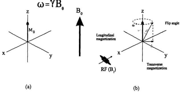
2.2). It is customary to choose the z-axis in the direction of the static magnetic field, Bq, as

shown in Fig. 2.2. If the nuclei are perturbed away from alignment with the static field, they

precess about the magnetic field (Fig. 2.1), like spiiming tops precessing around the direction

of the gravitational field [12]. The precessional frequency of the spins is called the Larmor

frequency, to, and it is proportional to the ma^etic field strength. The Larmor frequency is

25

= Y^o ' (2.1)

where y is the gyromagnetic ratio, which is unique for each magnetic isotope (y=2.675x10®

rad/sec/T for 'H). Detailed descriptions on concepts of MRI may be found in references

[13-17,29], a ) = Y B . Longitudinal magnetization

X

Figure 2.2 The effect of an RF pulse on spin magnetization, (a) net magnetization in equilibrium lies along the static field, (b) application of the RF filed causes a

2.1.1 The Bloch Equations

Bloch [18] gave an accurate phenomenological description of the time dependence of

the nuclear magnetization M(t) in the presence of an applied magnetic field B(t). The

nuclear magnetization M(t) is the source of the detected NMR signal. The NMR sample may

be thought of a system with input or stimulus B(t) and output or response M(t). The system

is characterized by parameters Mq, T,, and T,, where T, and T, are the longitudinal and

transverse relaxation associated with the sample (see section 2.1.2) and Mq is the equilibrium

magnetization. The behavior of the system output is governed by the bloch equation

d M -i. { M X + M v ) (Af -Af) z

= y M X B - — i ^

d t r, T . (2.2)

In general the B field of Eq. (2.2) consists of both the static field Bo= Bq z, and a

time-varying m^netic field Bi, called the RF field (Fig. 2.2). Eq. (2.2) may be written as a set of

27 d M M , = y(A//, -i = y ^ M B ^ - M B ) - —-i (2-3) d t •

dM^

M-M^

-f

From the set of Eqs. (2.3) the solution to the magnetization behavior of a sample for

a field = Bq, B^ = 0, and B^ = 0 is found as

MJjC)

A//0 = e '[Af^sin(&)oO + A/ cos(O)(,0] (2.4)

M,(0 = Mo - [M, - M;]e ' ,

where, My° and are the initial magnetization components of the sample at time t =0.

From the above equation, it can be seen that the longitudinal component of magnetization

constant. The transverse component rotates (precesses) about the z-axis at frequency o>o=yBo

and decays towards zero with a T, time constant. The solution to the Bloch equation will be

considered under three different scenarios:

1) Equilibrium state (i.e., no RF pulse has been applied to the system or there is a long delay

» T, from the last RF pulse). In this case and equal to zero, and Eq. (2.4) may be

simplified as,

MJj) = 0

= 0 (2.5)

M p )

where, (at equilibrium). From Eq. (2.5), the transverse magnetization components

of M are always zero (see Fig. 2.2(a)). In NMR experiments, the transverse magnetization components of M are the only components of the magnetization field that may be detected and, therefore, in equilibrium no signal is detected.

2) Application of a B, field with oscillation frequency to. In order to obtain transverse

magnetization components, M, and My, energy must be transmitted into the sample. This

is achieved by the application of the time-varying RF field, B, (i.e., a circular polarized field,

in the x-y plane). The radio frequency (RF) pulse (B, field) is the first step of a process that transforms the net equilibrium magnetization Mq, into a measurable NMR signal (i.e..

29 perturbs the magnetization away from its equilibrium condition aligned with the static field

as shown in Fig. 2.2). If an RF field with an oscillating frequency co close to the Larmor

frequency is applied to the sample, the net magnetization is perturbed from equilibrium. To

better understand the time variation of the magnetization, a rotating frame is considered. The

rotating frame of reference (as opposed to the laboratory frame) is a helpfiil method in

simplifying the complex precessional motion of the excited spins. The rotating firame

coordinate system is a frame of reference that rotates about the Bg field (z-axis) in the same

direction and with the same frequency as the circular polarized B, field. Therefore, the x and

y axis rotate ui synchrony with the B, field. The rotating firame may be better understood by

imagining a viewer standing at the origin of the coordinate system, and rotating at the same

rate as the magnetization vector is rotating about the z-axis. In this reference frame the

applied magnetic field Bq + B, is static. Consequently, the application of an RF pulse is seen to produce simple rotation or tilt of the net magnetization vector towards the transverse

plane, rather than a spiraling motion. Neglecting the relaxation terms for simplicity, Eq.

(2.2) in the rotating fi:ame may be written as [16]

dM

"dt' = yM X B

tff

(2.7)

and B, is the RF field applied perpendicular to the static field, Bq. Bj„is die resultant vector

shown in Fig. 2.3(a) operating on magnetization vector M. B, may be arbitrarily assigned

along the rotating x-axis, designated as the x'-axis in the rotating firame. From Eq. (2.6), it

can be seen that M in the rotating frame precesses about the The frequency of

precession around Bjn- is found as

= [(o)„ - o))2 + (Yfl,)'!" (2.8)

Z _Z

B

B

(a) (b)

Figure 2.3 Formation of Be(r in the rotating frame, (a) B,fr is not in the x-y plane when (i}?'(0o, (b) B^^f is along the x'-axis when o}=o)o.

31

3) Application of the RF field (B,) with an oscillation frequency Ci)=o)o (i.e., resonance

condition). From Eq. (2.7), at resonance (cd=o)o) B^^is equal to B, in the xy plane. Equation (2.8) at resonance may be simplified to

The degree of rotation of the magnetization from longitudinal magnetization aligned

in the z direction to the transverse magnetization is defined by a parameter called the flip

angle. For example, a 90° flip angle rotates the net magnetization from complete

longitudinal magnetization (equilibrium condition) to complete transverse magnetization.

The duration and magnitude of the RF pulse determines the flip angle. At resonance (&}=a)o),

the flip angle, a, may be determined by the amplitude of the RF pulse, B„ and its duration

Q = Y 5 , , f o r a ) = a ) o _(2.9)

T _P

(2.10)

0

=Yj5,Tp (rarf.) if for

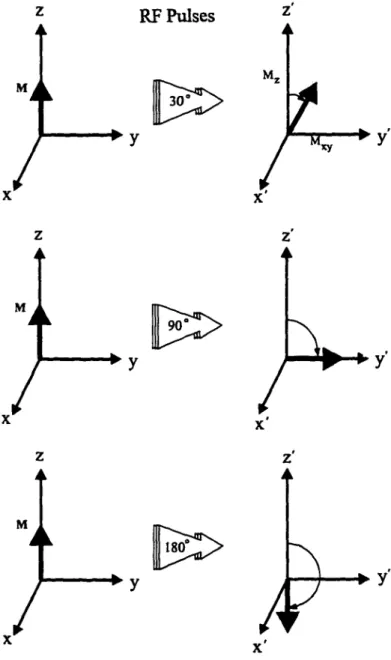
Figure 2.4 shows the effect of application of three RF pulses of 30, 90, or 180 degrees in a

RF Pulses m, lie—^ y _*y m 90 m 180 -• y

Figure 2.4 The effect of RF pulses with different flip angles on the net magnetization in the rotating frame.

33

2.1.2 Relaxation

Relaxation represents the process by which the spins respond after the perturbation

caused by the RF pulse. There are two major relaxation mechanisms: (1) longitudinal or

spin-lattice relaxation known as T, relaxation, and (2) transverse or spin-spin relaxation

known as T, relaxation. Both of the relaxation parameters, T, and T,, depend on certain

physical and chemical characteristics of the material. The imaging contrast associated with

different values of T, and T, for distinct tissues, as well as other factors such as the spin

densities, make MRI a unique and powerfiil technique in diagnostic imaging. Longitudinal

relaxation, or T,, pertains to the release of excess energy (absorbed by the spins from the RF

pulse) to the molecular environment or the lattice. The T, relaxation is best understood in

terms of the decay back to eqmlibrium magnetization, Mq, aligned with the static field. If Mq

is initially aligned with the z-axis, a 90° RF pulse will rotate it to the transverse plane,

resulting in zero longimdinal magnetization. The T, relaxation time is related to the time for

the recovery of the longitudinal magnetization and is represented as an exponential increase

of the longitudinal magnetization with a time constant of T,. Transverse relaxation, or T,,

pertains to a process that causes the spins to lose their phase coherence in the transverse

plane. Immediately after an RF pulse the transverse magnetization vectors from different

nuclei have identical phases, resulting in a strong MR signal. However, due to time-varying

field fluctuations between interacting spins, some nuclei experience a slightly weaker or

stronger magnetic fields. From Eq. (2.1), nuclei in a stronger magnetic field precess faster,

results in a reduction in the net transverse magnetization and, consequently, a signal loss.

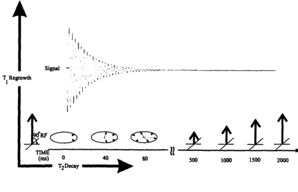
Figure 2.5 demonstrates the amplitude of the detected MR signal in relation to the T, and Tj

relaxation processes. A 90° RF pulse flips the net longitudinal magnetization to the

transverse plane. The transverse component of magnetization decays due to dephasing.

After some time the system recovers to its initial state (based on the T, value).

Another factor in causing dephasing of the transverse magnetization is spatial field

variations in the static field (field inhomogeneities). These field inhomogeneities (AB) result

in an even faster dephasing of the spins. The combination is referred to as Tj' relaxation and

is given by

_L ^ JL ^ YA^

T,* takes into account the dephasing factors of both spin-spin and static field variations

and, therefore, is shorter than T,. The loss of signal due to T2 or T,* is usually modeled

mathematically as an exponential decay as a fimction of time, although specific spatial

variations in field can lead to non-exponential decay. T, relaxation times generally range

firom tens to hundreds of milliseconds in biological samples, while T, relaxation times are

35 The m^netic field in which the spins are placed should be a homogenous and stable

Field, typically with a strength of 0.1-1.5 T for clinical imaging". In most modem MRI

systems this field is produced by superconducting magnets with a large (~60 cm) open bore.

The field inhomogeneities of the static magnetic field may be reduced by a process know as

shimming. Shimming coils inserted in the bore of a large static magnet are adjusted until

acceptable homogeneity in the magnetic field is produced.

Signal T Regrowlh 9(fRF A

CZJ)

CD> CS5

.J^AAA.

Figure 2.5 T, and Tj relaxations are simultaneous processes with Tj being shorter than T,.

- T is the abbreviation for Tesla, a measure of field strength. The earth's magnetic filed is approximately 0.00005 T at the equator.

2.1.3 Free Induction Decay

The free-induction-decay (FID) represents the signal produced after the application

of an RF pulse. For identical nuclei in a homogenous magnetic field, the FID signal

oscillates at the Larmor frequency, and decays exponentially to zero due to the T,* relaxation

processes. The precise resonance frequency of a nucleus depends on its local chemical

enviroiunent. Variations in frequency due to different chemical environments within a

molecule, called chemical shift, is the basis of NMR spectroscopy. A ID Fourier transform

of an FID signal (the frequency spectrum of the FID) reveals the resonance peaks of the

nuclei within the sample. The area under the peak is proportional to the density of each

nuclei. The spectrum may be used in determining the chemical makeup of a sample. In most

biological specimens, the spectrum is dominated by the hydrogen nuclei in water and fat.

These nuclei have resonance frequencies that differ by approximately 3.5 ppm. As a result,

it is possible to construct images that reveal the spatial distribution of either fat or water

37

2.2 BASIC PRINCIPLES OF IVfRT

The FID signal measured in an NMR experiment does not provide any spatial

information about the nuclei within the sample. In NMR imaging^ spatial information is

encoded by having the nuclei at different locations experience different magnetic fields. This

is done by use of gradient magnetic fields. The purposeful activation of specialized gradient

coils creates predictable variations in the main magnetic field and allows spatial encoding

of the MR signal. The gradient is defined as the rate at which magnetic field strength

changes with position and is usually expressed in millitesla per meter (mT m"') or gauss per

cm (G cm"'), where 10 mT m''=l G cm"'. The magnitude of the gradient fields vary linearly

with distance in the three coordinates of x, y and z, while the direction of the field points in

the z direction, the same durection as the static field. The total magnetic field applied can be

described mathematically by

Bit) = + xG/f) + yG^it) + zG^(f)] T (2-12)

where G^, Gy, and G^ are time-varying gradient values. Equation (2.12) is an approximation

over a limited spatial extent (the true

B(t)

*B

^ By the mid-1980s the term NMR imaging had been largely dropped and replaced by MRI, partially because of patient's concern over the nuclear terminology.

imaging methods, one gradient is applied along with the RF pulse to select a slice, a second

gradient encodes location along one in-plane dimension in the frequency of the MR signal,

and a third gradient encodes location along the other in-plane dimension in the phase of the

MR signal.

2.2.1 Slice Selection

The initial step in MRI is the localization of the excitation to a region of space within

the sample. This is accomplished through the use of frequency-selective excitation (RF

pulse) in conjunction with the slice selection gradient. Although the slice, frequency, and

phase gradients are interchangeable in MRI depending on the desired slice orientation, in this

dissertation they will be referred to as the G^, G^, and Gy gradients, respectively. With the

application of the slice gradient, the resonance frequencies of the tissue protons become

linearly related to position along the z-axis, such that individual resonance frequencies

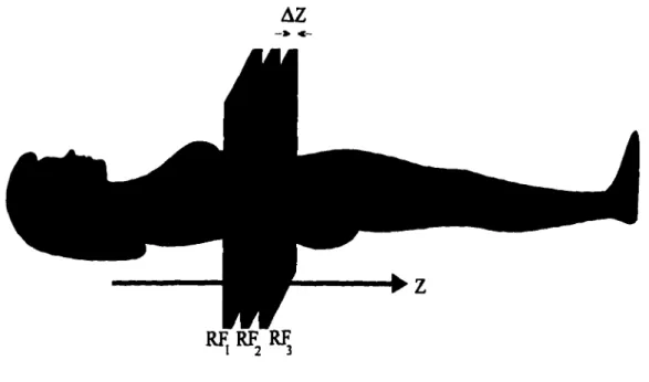
correspond to individual planes of nuclei, perpendicular to the z-axis. If an RF pulse is

applied simultaneously with the slice selection gradient, only nuclei corresponding to the

frequencies of the RF pulse resonate. These slices may be visualized as in Fig. 2.6. The

location of the individual slice along the z-axis and the thickness (AZ) are determined by the

carrier frequency of the RF pulse, co^ the bandwidth of the RF pulse, Aq, and the amplitude

Figure 2.6 Application of RF pulses at different frequencies results in excitation of different slices along and perpendicular to the z-axis.

The slope of the line in Fig. 2.7(a). is given by the gyromagnetic ratio times the

amplitude of the slice gradient, and is partially responsible for the thickness of the excited

slice. As shown in Fig. 2.7, when a)=o)j, a slice centered at z=

Z

parameter contributing to the slice thickness is the bandwidth of the RF pulse, which is

determined by the shape (envelope) of the pulse as shown in Fig. 2.7(b) (i.e., a faster

oscillating sine flmction in the time domain has a larger bandwidth in the frequency domain,

and vise versa). The choice of a sine function for the RF pulse envelope results in uniform

excitation of a band in the frequency domain. In practice, only a finite duration RF pulse (a

truncated sine envelope) may be applied to the sample. Since the Fourier transform of a

Other shapes of envelopes may be used that result in a more uniform excitation in the

frequency domain [44]. The choice of slice thickness affects the quality of the reconstructed

image. Thicker slices provide more signal per voxel, while thinner slices produce less partial

volume averaging and, therefore, better resolution.

CO = YB^+YzG^ AO) =

YG,

(b)

Figure 2.7 Slice selection procedure, (a) Graph of (o vs z, shows the relationship between the carrier frequency of the RF pulse, with the location of excited slice, (b)

Application of a sine shaped RF pulse with the slice gradient, excites a nearly uniform frequency distribution (slice profile).

41 2.2.2 Spatial Encoding

Once a cross-section or slice with a thickness, Az, is excited, the gradients and G,,

are activated to further encode the rotating transverse magnetization. One of the in-plane

dimensions is encoded by changes in frequency, whereas the other is encoded by differences

in phase. From the Larmor relationship, with the application of the x and y gradients, the

frequency for a nuclei at position (x,y) and time (f), is given by

= Y^o ^ yxGJ,t') + yyGp'). (2.13)

The phase 4) acquired up to time t is given by

t

• (2.14)

0

The total detected MR signal from the nuclei at all spatial positions is given by

5(0 = R e { f f a ( x j > ) e d x d y } , (2.15)

where o(x,y) represents the MR signal strength, which includes effects due to the spin

density distribution and the T, and Tj relaxation effects. Combining Eqs. (2.14) and (2.15)

i

-jyxfG^t')dt' -jyyjfa/t'wt'

e''^''J'J'a(x,y)e ' e ' dxdy . (2.16)

The actual MR signal is obtained by quadrature demodulation off the leading exponential

(i.e., demodulation of a complex signal from the Larmor carrier frequency), which yields the

signal s'{t) = j'Ja(x,y)e dxdy , (2.17) where. 0 and (2.18) t 271 0

Equation (2.17) is recognized as the 2D Fourier transform of o(x,y) with the Fourier

conjugate variables k, and ky. The complex acquired MR data is a measurement of

"space". K-space is simply the 2D Fourier transform of the MR image. The path taken in

k-space as a function of time is defined by Eq. (2.18). From Eq. (2.18) the integrals of the

gradients over time define the scanning path through the k-space. An example of a path

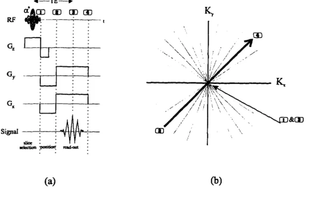
taken through the k-space is shown in Fig. 2.8. From points ® to (D the x and y gradients

43 echo time, TE, is the time between the center of the RP pulse and the center of the readout

period (i.e., the point where ky=0). By repeating the pulse sequence of Fig. 2.8 with changing

amplitudes for the y-gradient, the complete k-space may be measured as a series of lines in

k-space. This is referred to as the Fourier method or the rectilinear scan method.

Alternatively, both gradients can be controlled in such a fashion that the Fourier data are

scanned as a series of radial lines. This is known as the radial-scan method. An example of

a gradient-echo pulse sequence with radial-scan acquisition is shown in Fig. 2.9. The slope

of the radial line is determined by the ratio of the and Gy gradients. By proper selection

of the and Gy gradients in a series of acquisitions, the complete k-space may be scaimed

in a radial-line maimer. Data acquired with such pulse sequences may then be reconstructed

via the filtered backprojection algorithm.

The signal S'(t) during the read-out period is sampled, digitized and stored for image

reconstruction. The trajectory taken through k-space, defined by the x and y gradients,

determines the order that data are collected. Based on the MR acquisition method, the MRJ

reconstruction system uses the collected data to reconstruct the resulting images. Two

standard reconstruction algorithms are the 2D Fourier transform and filtered backprojection.

The real-time MRI reconstruction system presented in this dissertation uses the 2D FFT

algorithm for reconstructing data that are acquired on a rectilinear grid, and the filtered

backprojection algorithm for data that are acquired on a polar grid. These algorithms, which

are discussed in the next chapter. •< TE • «IlX) (D CB CB Signal

3

leleccioa positiaiC icadKxit

CD XI ' \ s \ \ \ \ \ UJ OD

(a) Gradient Echo Pulse Sequence

(b) k-space Trajectory

Figure 2.8 Scanning the k-space. (a) The pulse sequence for a typical gradient-echo sequence, (b) The corresponding trajectory path taken through the k-space, from (D

on the z-axis (center of k-space), pre-positioned to (D, and a horizontal read-out from <D to ® with a maximum echo at point ®.

45 •4 TE • "ACT) (X) CE (D RF

T

u

u

\

'\ , ••

\

X

\!/y.

w

.J

^

/

(a)

Figure 2.9 Gradient-echo pulse sequence for radial-scan, (a) The gradient-echo pulse sequence for a typical radial-scan in k-space. (b) The corresponding trajectory path

taken through the k-space, from ® on the origin (center of k-space), pre-positioned to and a radial read-out from (D to ® with a maximum echo at point ®.

2..1 THE NMR SIGNAL DETECTION SYSTEM

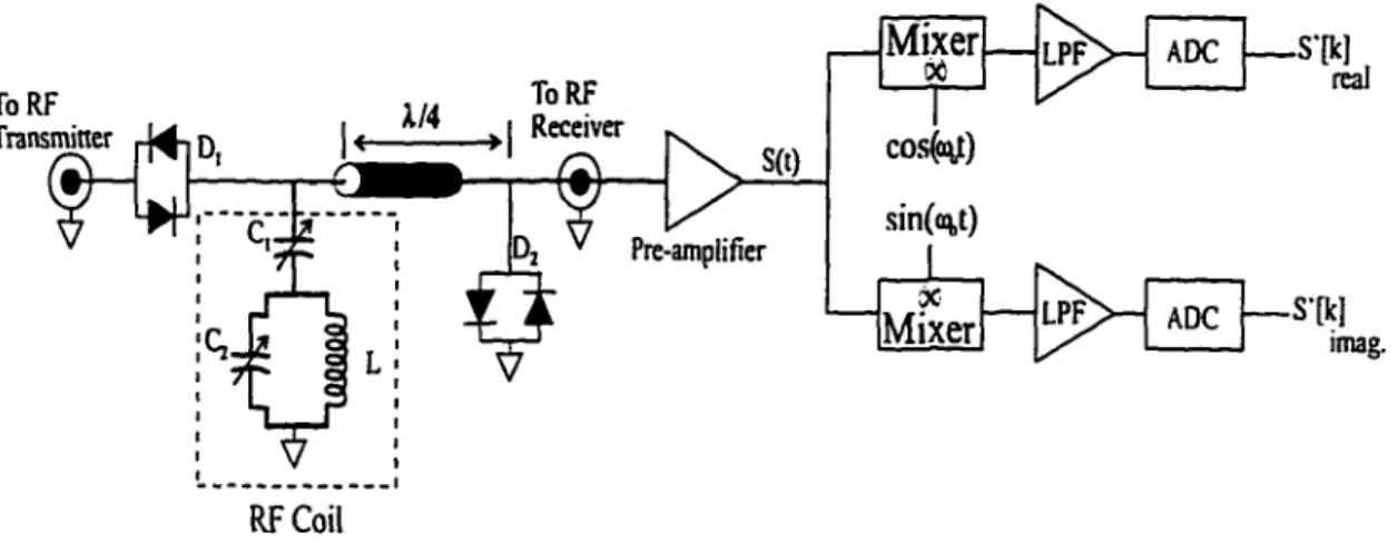
The MR signal detection is achieved through the use of an RF coil. Figure 2.10 shows

an RF transmitter/receiver coil with the RF signal processing circuitry. The RF coil, which

usually surrounds the sample, is an antenna that transmits an oscillating B, field and receives

the NMR signal by an EMF induced in the coil by the precessing transverse magnetization

of the sample (Faraday effect). The RF coil and the signal processing/detection circuitry are

disciissed in this section. For discussions on the RF transmitter system the interested reader

is referred to references [13] and [42-43].

2.^A RF Coil

The RF coil has two primary functions: (1) transfer RF power to the sample and (2)

detection of the resulting signal from the nuclear spin precession. The RF coil should be an

efficient transmitter as well as a receiver. For imaging it is also desired to have uniform

spatial excitation (homogeneous B, field). The RF coil is tuned to broadcast or receive over

a certain frequency range. The operating frequency of the RF coil is tuned by the parallel

capacitor Q shown in the LC circuit of the RF coil (Fig. 2.10). Cj is referred as the tuning

capacitor. The resonant frequency of the circuit is given by

47

Mixer

LPF

AIX:

.-a

LPF

ADC

Mixer

Figure 2.10 The RF coil receiver and the quadrature demodulation circuit.

The capacitor C, (matching capacitor) is put in series to the parallel LC pircuit to

change the impedance of the RP coil. The matching capacitor is adjusted to match the

impedance of the RF coil to the output impedance of the RF transmitter circuitry (not shown

here), which is typically 50 Q. The crossed diodes of D, and Dj function as switches for the

transmit and receive modes of the RF coil. During the high power RF pulse, the diode pair

D, have a relatively small "on" resistance, therefore conducting the RF pulse to the RF coil.

However, during signal detection the low-level voltages induced in the RF coil leave the

detection circuitry.

The protection of the pre-amplifier during the transmit pulse is achieved by the special

properties of a quarter wavelength (A/4) transmission line as shown in Fig. 2.10 [27]. The

input impedance of a quarter wavelength line terminated by impedance 7^ (impedance of the

crossed diodes Dj) is given by Zj„ = Z^Zl, where Zq is the impedance of the quarter

wavelength line. During the transmit pulse, the crossed diodes Dj are "on" which results in

a low impedance, Zl (compared to Zo), therefore, the input impedance Zj^ appears high.

During the low-level signal detection, the D, pair are "off", resulting in a high Z^, and

therefore, low input impedance, Z,„.

2.3.2 Signal Processing

The relatively small output voltage of the RF coil is first amplified by a pre-amplifier

(Fig. 2.10). This signal (S(t) in Eq. 2.16) consists of a distribution of frequencies centered

around or near the resonant frequency (Oq (e.g., 200 MHz for a 4.7T system). A quadrature

detection (demodulation) method is used to obtain the real and imaginary components of the

MR signal S'(t). The demodulation brings the center of the real and imaginary signals'

distribution of frequencies to zero, but leaves the distribution of frequencies unchanged.

The quadrature demodulation is achieved by first splitting the amplified signal into two

49

out of phase by 90° (cos((»)ot) and sin(cOot)). The output signals of the multipliers (mixers)

contain the demodulated real and imaginary components of the NMR signal (centered at zero

frequency) as well as signals centered at a frequency (see [28] for mathematical

derivation). The low pass filters (LPF) are used to pass only the demodulated real and

imaginary components of S'(t) (Eq. 2.17). Each channel is then digitized to generate

CHAPTERS

MRI ACQUISITION AND RECONSTRUCTION METHODS

Magnetic resonance imaging is a very rapidly developing modality. Although only a

few examples of MRI imaging methods are presented in this dissertation, there are many

options for generating images in terms of manipulating field gradients and RF pulses. In this

chapter a conventional MR imaging acquisition method, namely spin-echo, and two fast

acquisition methods, gradient-echo and echo-planar-im^ing (EPI), are reviewed. Spin-echo

and gradient-echo fall into the multiple-shot acquisition category, whereas EPI is an ultra-fast

single-shot acquisition technique. Spin-echo or gradient-echo may be employed in

rectilinear-scan or radial-scan, whereas EPI can be implemented as either a rectilinear-scan

or a spiral-scan method. Data acquired using the rectilinear-scan method are reconstructed

via the 2D Fourier transform algorithm, whereas data acquired form the radial-scan or

spiral-scan techniques are reconstructed via the filtered backprojection algorithm'. The above MR

acquisition methods, as well as the aforementioned reconstruction algorithms, are the topics

of discussion in this chapter.

' Data acquired using the radial-scan or the spiral-scan methods may also be interpolated to a rectilinear grid and then reconstructed via the standard 2D Fourier transform

51

3.1 MTJLTTPLE-SHOT MR ACQUISITION METHODS

In the most common multiple-shot MR acquisition methods, one line of k-space is

acquired for every RF pulse excitation". The time between successive excitation of the spins

is called TR (repetition time). The required time to complete one 2D scan is equal to the

repetition time multiplied by the total number of acquired lines, Ny For example, if TR=1.0

second, and Ny=256, the total acquisition time for one frame of data is 4.2 minutes.

Therefore, for an equal number of data lines acquired per frame, the total scan-time is

directly proportional to TR. Reduced imaging time is the main motivation for the

development of scan methods that use relatively short repetition times.

3.1.1 Spin-Echo

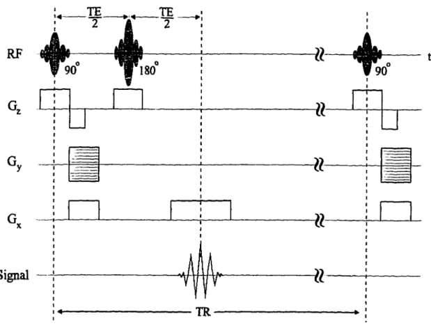
The most common MRJ technique is spin-echo. In its most basic form, the spin-echo

pulse sequence consists of 90° and 180° RF pulses, separated in time by a TE/2 time interval

[13-17]. An example of a spin-echo pulse sequence is shown in Fig. 3.1. The spins are

rotated into the transverse plane by the 90° RF pulse. The spins then start to dephase due to

the Tj' relaxation. A 180° RF pulse applied at a time TE/2 after the 90° RF pulse can be

shown to reestablish (refocus) phase coherence at a time TE after the 90° RF pulse. The 180°

^ Some multiple-shot acquisition methods acquire more than one line of k-space for each RF excitation.

TR

Figure 3.1 Spin-echo pulse sequence for raster-scan.

RF pulse flips the partially dephased magnetization over in one direction such that the faster

precessing spins will catch up with the slow ones at time TE. The refocusing takes place

such that the dephasing effects from both static magnetic field inhomogeneities and the

added gradient fields are canceled at TE, the echo time. Consequently, the signal is Tj

weighted, rather than Tj* weighted. With appropriate acquisition timing parameters of TR

53 or the spin density. In spin-echo imaging the signal strength a(x,y) of Eq. (2.17) is related

to the relaxation parameters T,, T,, and the spin density Po(x,y) by

TE TR

a(x^) = Apgixo') (e - e

where A is a proportionality constant.

From the above equation it can be seen that the parameters TE and TR may be selected

to obtain weighted images as described in Table 3.1. For example in T,-weighted images,

tissues with short T,, such as fat, appear bright, whereas tissues with long T„ such as many

tumors and edema, appear dark. For T^-weighted images, tissues with long Tj, such as

tumors and cysts, appear bright, whereas tissues with short Tj, such as muscle and liver,

appear darker. In the case of proton density-weighted images, the tissues with higher

concentration of protons, appear brighter. It should be noted that both Tj-and-Ti-weighted

images have proton density contributions as well.

Table 3.1. Contrast enhancement in spin-echo by manipulation of TR and TE.

TR TE Resulting Imaee

short (TR - T,) short (TE < Tj) T,-weighted

long (TR» T,) short (TE < Tj) proton density-weighted

Gradient-echo sequences are sequences bearing acronyms such as FLASH, FISP,

FAST, SSFP, and GRASS [22,29] that employ gradient reversal rather than a 180° pulse in

order to generate an echo signal. The gradient-echo sequences typically use small flip angle

RF pulses, a, where a is a flip angle of less than 90°. An example of a gradient-echo pulse

sequence was shown in Fig. 2.8. As shown in the figure, the reversal of the frequency

gradient G^ produces a gradient-echo or refocusing at (D. The precession frequency of the

spins (due to the application of the x-gradient) at ® is o)^=y(Bo - xGJ. By applying a

gradient reversal with an amplitude of -Kj^ such that the area under the x-gradient waveform

from points ® to @ is equal in magnitude to the area of the same gradient from points <D to

the dephasing of the spins due to the gradient is canceled out. The reversal of the

x-gradient to an amplitude of +Gx from @ to ® causes the spins to refocus at (D. Since the

gradient-echo sequences lack a refocusing RF pulse, the effects of static field

inhomogeneities are not removed from the detected signal. Therefore, unlike the spin-echo

pulse sequences, the signal intensity is determined from the shorter T2* relaxation.

The flip angle used in the gradient-echo pulse sequences may be freely varied. When

a 90° RF pulse is used, all of the net magnetization is rotated to the transverse plane. This

produces a strong signal, but leaves no longitudinal magnetization for the successive RF

excitation pulses (saturated signal). However, when smaller flip angles are used, the

55 next RF pulse can operate on a significant longitudinal magnetization component. Thus,

faster imaging sequences (compared to spin-echo) are possible. For example, in FLASH, the

optimal flip angle, (Ernst angle), that maximizes the signal amplitude for a given TR and

a material with a specific T, is given by

-77?

= cos-'[exp(—)] . (3 2)

^ I

Depending on the pulse sequence, the pulse sequence parameters TR, TE, and a, and

the tissue parameters T„ T,, and proton density, various weighted images may be obtained.

Gradient-echo techniques may be utilized to obtain complete k-space scans in as short as one

second (i.e., a 128 x 128 scan with TR = 8 ms). Although this is a great improvement over

the spin-echo scan time, it is still long compared to many physiological motions in the body

3.2 SINGLE-SHOT MR ACOIJTSTTTQN MFTHODS

The fastest MR acquisition methods are those that sample the entire k-space in one

acquisition (i.e., single-shot). The total acquisition time of such methods must be shorter than

the exponential T, decay of the transverse magnetization to avoid substantial signal loss.

Two methods of single-shot acquisition are echo-planar imaging (EPI) and spiral-scan echo

planar imaging (SEPI). EPI and SEPI are different only in their gradient waveforms, which

results in different trajectories through the k-space. Examples of these single-shot pulse

sequences are shown in Fig. 3.2. The RP excitation and slice selection gradient (not shown)

are similar to the conventional MR acquisition methods (i.e., spin-echo or gradient-echo).

The first two sequences of Fig. 3.2 are characterized by a series of gradient reversals

in the readout direction. Each gradient reversal creates a gradient echo with the second half

of one readout period being rephased by the first half of the following readout period. In

order to sample the k-space along a horizontal line, the phase gradients are pulsed in what

is called a "blip" pulse shape^. In this version of EPI, called blipped-echo-planar (BEPI),

multiple gradient pulses of very short duration (blips) are applied in the phase encoding

direction. Each phase encoding blip applies a small amplitude gradient pulse prior to each

sampling period. The phase gradient is off during signal detection. The read gradient for the

^ The original EPI method had a constant but small phase gradient which was left on during the pulse sequence. As a result the k-space was traversed in a sinusoidal manner.

57 BEPI is a sinusoidal wave, with the actual readout segments allocated to the upper and lower

portions of the wave. Another version of BEPI is MBEPI

(modified-blipped-echo-planar-imaging), which employs a trapezoidal shaped read gradient. The readout segments of this

gradient are allocated to the flat top and bottom portions of the trapezoidal wave. The

advantages and disadvantages of BEPI and MBPI methods are discussed in the next section.

The third single-shot acquisition method shown in Fig. 3.2(c) is spiral-scan echo-planar

imaging (SEPI). The spiral-scan starts from the center of the k-space (low spatial frequency)

and spirals outward (towards high spatial frequencies). The spiral-scanned data may be

sampled at points falling on radial lines. While the and Gy gradients' oscillation

frequency defines the rotational speed of the spiral motion, its amplitude specifies the gap

between each spiral and ultimately the extent of the spiral-scan. G^ and Gy may be selected

to scan the k-space for a suitable data acquisition format (e.g., 32 spirals in a total acquisition

I I I I I I I •

J1

I I I I I I I

Figure 3.2 Single-shot acquisition methods and the location of sample points in k-space. (a) Blipped echo-planar imaging, (b) Modified blipped echo-planar imaging,

59

3.2.1 Single-Shot Data Acquisition Concerns

As seen in Fig. 3.2(a), the gradient amplitude is changing during the readout segment.

Consequently, from Eq. 2.18 the trajectory speed in the k, direction is not constant in time,

or in other words, the trajectory gets slower for points farther from the ky axis, and grows

faster for points closer to the ky axis. Therefore, a un