The University of Sydney Business School The University of Sydney
BUSINESS ANALYTICS WORKING PAPER SERIES
Efficient estimation of parameters in marginal
in semiparametric multivariate models
Valentyn Panchenko
Artem Prokhorov
March 2016
Abstract
We consider a general multivariate model where univariate marginal distributions are known up to a common parameter vector and we are interested in estimating that vector without assuming anything about the joint distribution, except for the marginals. If we assume independence between the marginals and maximize the resulting quasi-likelihood, we obtain a consistent but inefficient estimate. If we assume a parametric copula (other than independence) we obtain a full MLE, which is efficient but only under correct copula specification and badly biased if the copula is misspecified. Instead we propose a sieve MLE estimator which improves over OMLE but does not suffer the drawbacks of the full MLE. We model the unknown part of the joint distribution using the Bernstein-Kantorovich polynomial copula and assess the resulting improvement over QMLE and over misspecified FMLE in terms of relative efficiency and robustness. We derive the asymptotic distribution of the new estimator and show that it reaches the semiparametric efficiency bound. Simulations suggest that the sieve MLE can be almost as efficient as FMLE relative to QMLE provided there is enough dependence between the marginals. An application using insurance company loss and expense data demonstrates empirical relevance of the estimator.
JEL Classification: C13
Keywords: sieve MLE, copula, semiparametric efficiency
BA Working Paper No: BAWP-2016-04
Efficient estimation of parameters in marginals
in semiparametric multivariate models
∗
Valentyn Panchenko
†Artem Prokhorov
‡Mar 2016
Abstract
We consider a general multivariate model where univariate marginal distributions are known up to a common parameter vector and we are interested in estimating that vector without assuming anything about the joint distribution, except for the marginals. If we assume independence between the marginals and maximize the resulting quasi-likelihood, we obtain a consistent but inefficient estimate. If we assume a parametric copula (other than independence) we obtian a full MLE, which is efficient but only under correct copula specification and badly biased if the copula is misspecified. Instead we propose a sieve MLE estimator which improves over QMLE but does not suffer the drawbacks of the full MLE. We model the unknown part of the joint distribution using the Bernstein-Kantorovich polynomial copula and assess the resulting improvement over QMLE and over misspecified FMLE in terms of relative efficiency and robustness. We derive the asymptotic distribution of the new estimator and show that it reaches the semiparametric efficiency bound. Simulations suggest that the sieve MLE can be almost as efficient as FMLE relative to QMLE provided there is enough dependence between the marginals. An application using insurance company loss and expense data demonstrates empirical relevance of the estimator.
JEL Classification: C13
Keywords: sieve MLE, copula, semiparametric efficiency
∗Helpfull comments of seminar participants at University of Toronto, University of Pittsburgh, University
of New South Wales, Concordia University, QMF, International Panel Data and FESAMES are gratefully acknowledged.
†Economics at the Australian School of Business, University of New South Wales, Sydney NSW 2052,
Australia; email: valentyn.panchenko(at)unsw.edu.au
‡University of Sydney Business School, Sydney NSW 2006, Australia; email:
1
Introduction
Consider anm-variate random variableY with joint pdfh(y1, . . . , ym). Letf1(y1), . . . , fm(ym)
denote the corresponding marginal pdf’s. Assume that the marginals are known up to a parameter vector β, where β collects all the distinct parameters in the marginals. The
de-pendence structure between the marginals is not parameterized. We observe an i.i.d. sample
{yi}Ni=1 ={y1i, . . . , ymi}Ni=1 and we are interested in estimatingβ efficiently without assuming
anything about the joint distribution except for the marginals.
As an example consider the setting of a standard panel (small T, large N). We have
a well specified marginal for each of T cross sections (e.g., logit models, duration models,
stochastic frontier models, etc.) and we are interested in efficient estimation of the parameters in the marginal distributions with no apriori knowledge of the form or strength of dependence between them. This or similar setting is often encountered in microeconomic and actuarial applications (see, e.g, Winkelmann, 2012; Amsler et al., 2014; Frees and Valdez, 1998). In finance, a similar setting arises in the so called SCOMDY models and in other multivarariate GARCH-type models, where interest is in estimation of univariate conditional distribution parameters while the error terms are allowed to have arbitrary dependence (Chen and Fan, 2006a,b; Hafner and Reznikova, 2010).
However, recent literature on semiparametric copula models has focused on the case when the marginals are specified nonparametrically and the copula function is given a parametric form (see, e.g., Chen et al., 2006; Segers et al., 2008), which is an appropriate setting for many financial applications where it is important to parameterize dependence. In our setting, dependence is used solely to provide more precision in estimation of marginal parameters so
we study the converse problem.
We will use the well known representation of log-joint-density in terms of log-marginal-densities and the log-copula-density:
lnh(y1, . . . , ym;β) = m
X
j=1
lnfj(yj;β) + lnc(F1(y1;β), . . . , Fm(ym;β)), (1)
where c(· · ·) is a copula density and Fi(·) denotes the corresponding marginal cdf. This
decomposition is due to Sklar’s (1959) theorem which states that any continuous joint distri-bution can be represented by a unique copula function of the marginal cdf’s.
It is well understood that the parameters of the marginals can be consistently estimated by maximizing the likelihood under the assumption of independence between the marginals – this is the so called quasi maximum likelihood estimator, or QMLE. The copula term in (1) is zero in this case because the independence copula density is equal to one. However, QMLE is not efficient if marginals are not independent and for highly dependent marginals, the efficiency loss relative to the correctly specified full likelihood MLE is quite large. Joe (2005), for instance, reports up to 93% improvements in relative efficiency over QMLE in simulations when the full likelihood is correctly specified.
The situation when using copula terms in the likelihood does not improve asymptotic efficiency over QMLE is known as copula redundancy. Prokhorov and Schmidt (2009) derived a necessary and sufficient condition for copula redundancy and showed that such situations are very rare. Essentially, a parametric copula is redundant for estimation of parameters in the marginals if and only if the copula score with respect to these parameters can be written as a
linear combination of the marginal scores – a condition generally violated for most commonly used parametric copula families and marginal distributions. As a result, significant efficiency gains remain unexploited.
An alternative that is more efficient asymptotically is a fully parametric estimation of the entire multivariate distribution by full MLE. This means assuming a parametric copula specification in addition to the marginal distributions. It is now well understood that, unlike QMLE, FMLE is generally not robust to copula misspecification. That is, the efficiency gains will come at the expense of an asymptotic bias if the joint density is misspecified. Prokhorov and Schmidt (2009) point out that there are robust parametric copulas, for which the pseudo MLE (PMLE) using an incorrectly specified copula family leads to a consistent estimation. However, copula robustness is problem specific and some robust copulas are robust because they are redundant. So finding a general class of robust non-redundant copulas remains an unresolved problem.
In this paper we address this problem using a semiparametric approach. That is, we investigate whether we can obtain a consistent estimator ofβ, which is relatively more efficient
than QMLE, by modelling the copula term nonparametrically. We use sieve MLE (SMLE) to do that. The questions we ask are whether a sieve-based copula approximator is the robust non-redundant alternative to QMLE and PMLE and what is the semiparametric efficiency bound for the SMLE ofβ. So our paper relates to the literature on sieve estimation (see, e.g.,
Ai and Chen, 2003; Newey and Powell, 2003; Bierens, 2014) and on semiparametric efficiency bounds (see, e.g., Severini and Tripathi, 2001; Newey, 1990).
con-sistency, asymptotic normality and semiparametric efficiency. Section 3 contains simulation results, confirming the significant efficiency gains permitted by SMLE. Section 4 presents an insurance application. Section 5 contains concluding remarks.
2
Sieve MLE
Denote the true copula density by co(u), u = (u1, . . . , um), and denote the true parameter
vector byβo. Letβobelong to finite dimensional spaceB ⊂Rpandco(u) belong to an
infinite-dimensional space Γ ={c(u) : [0,1]m →[0,1],R[0,1]mc(u)du= 1,
R
[0,1]m−1cJN(u-`)du-`= 1,∀`},
where u-` excludes u`. These conditions reflect that any copula is a joint probability
distri-bution on the unit cube [0,1]m with uniform marginals. Given a finite amount of data,
optimization over the infinite-dimensional space Γ is not feasible. The method of sieves is useful for overcoming this problem. Compared to other nonparametric methods such as ker-nels, local linear estimators, etc., the method of linear sieves is also quite simple – the infinite dimensional optimization is reduced to a regular parametric MLE.
Define a sequence of approximating spaces ΓN, called sieves, such that
S
NΓN is dense
in Γ. Optimization is then restricted to the sieve space. Grenander (1981) is credited for observing that the MLE optimization, which is infeasible over an infinite dimensional space, is remedied if we optimize over a subset of the parameter space, known as the sieve space, and then allow the subset to grow with the sample size (see, e.g., Chen, 2007, for a survey of sieve methods).
for approximating univariate functions on [0,1]. To generalize them for multivariate copula
setting, we can write them in a tensor product form as follows:
ΓN = cJN(u) = JN(1) X k1=1 · · · JN(m) X km=1 ak1,...,kmAk1(u1)×. . .×Akm(um), u∈[0,1]m, Z [0,1]m cJN(u)du= 1, Z [0,1]m−1 cJN(u-`)du-` = 1, ∀` , JN(`) → ∞, J (`) N N →0, l= 1, . . . , m
where {Ak`} are known univariate basis functions, {J
(`)
N } is the number of basis elements in
each direction ` and {ak1,...,km} are unknown sieve coefficients. Commonly used examples of
basis functionsAk(u) include power series, trigonometric polynomials, Fourier series,
Cheby-shev polynomials, splines, wavelets, neural networks and many others (see, e.g., Chen, 2007). The number of sieve elements in the tensor sieve JN(1) × · · · ×JN(m) can be viewed as the smoothing parameter analogous to the bandwidth in a kernel estimation.
One of the challenges with the tensor product sieve is ensuring that the resulting sieve is the proper copula pdf, that is, it is non-negative, integrates to one and the marginals are uniform. Exponential or quadratic transformations are used often to ensure positivity and division by a normalizing constant is used to ensure that the sieve integrates to one (see, e.g., Chen et al., 2006). However, it is difficult to find an appropriate normalisation to ensure that all marginals are uniform. Moreover, the properties of the normalised objects, namely, the rates of convergence, may differ from the original sieve and may not be easy to derive. An alternative which does not require any transformation to satisfy the proper copula conditions is the Bernstein-Kantorovich polynomial (see, e.g., Sancetta and Satchell, 2004). In addition
to this, the parameters of the Bernstein-Kantorovich sieve have a meaningful interpretation.
2.1
Bernstein-Kantorovich Sieve
The Bernstein-Kantorovich sieve is a tensor product sieve which uses β-densities as basis
functions; it can be written as follows:
cJN(u) = (JN) m JN−1 X v1=0 · · · JN−1 X vm=0 ωv m Y l=1 JN −1 vl uvl l (1−ul)JN−vl−1, (2)
where ωv denotes parameters of the polynomial indexed by multi-index v = (v1, . . . , vm)
such that 0 ≤ ωv ≤ 1 and
PJN−1
v1=0 · · ·
PJN−1
vm=0ωv = 1. These restrictions ensure that the
above equation is a proper density. The interpretation of the coefficients ωv is that they are
probability masses on an JN × · · · ×JN grid (see, e.g., Zheng, 2011; Burda and Prokhorov,
2014).1 In order to ensure thatc
Jm
N(u) is a copula density, i.e. that its marginals are uniform,
we further require thatP
v-`ωv = 1/(JN)
m−1, where multiple summationsP
v-` are performed
over all elements ofv except v`, `= 1. . . m.
The weightsωv can be viewed as a multivariate empirical copula density estimator, ωv=
1
N
PN
i=1I(ui ∈Hv), where ui = (ui1, . . . , uim)∈[0,1]
m,
I(·) is the indicator function and
Hv = v1 JN ,v1+ 1 JN × · · · × vm JN ,vm+ 1 JN . (3)
So the Bernstein-Kantorovich polynomial sieve has the interpretation of a smoothed copula histogram where smoothing is done by the product of β-densities. Alternatively, it can be
1For simplicity we assume that J
N is the same for every dimension `, but this assumption can be easily
viewed as a mixture of the product ofβ-densities in u.
Sancetta (2007) derives the rates of convergence of the Bernstein-Kantorovich copula to the true copula. Petrone and Wasserman (2002) and Burda and Prokhorov (2014) established consistency of the Bernstein-Kantorovich polynomial when used as a prior on the space of den-sities on [0,1]m in a Bayesian framework. Ghosal (2001) and references therein discuss the rate of convergence of the sieve MLE based on the Bernstein polynomial (only for one-dimensional densities). Uniform approximation results for the univariate and bivariate Bernstein density estimator can be also found in Vitale (1975) and Tenbusch (1994). As JN → ∞, cJN(u) is
known to converge to the probability limit of the empirical copula estimator at every point on [0,1]m where the limit exists, and if it is continuous and bounded then the convergence is
uniform (see, e.g., Lorentz, 1986).
This sieve is particularly attractive in our multivariate settings because of the uniform rate of convergence results available forcJN and because of the empirical copula interpretation of
ωv. The former ensures a relatively fast convergence compared to other tensor product sieves,
which we observe in simulations, while the latter permits natural adaptive dimension reduction based on droppingωv’s which correspond to sparsely populated grid cells.
2.2
Asymptotic Properties
We can now write the sieve for Θ = B ×Γ as ΘN = B×ΓN, where ΓN contains a generic
γ =ωv. Let θ = (β0, c), then the sieve MLE (SMLE) can be written as follows ˆ θ = arg max θ∈ΘN N X i=1 lnh(yi;θ) (4)
In essence, an indimensional problem over a space of functions is reduced to a finite-dimensional problem over a sieve of that space. As pointed out in sieve MLE literature (see, e.g., Chen, 2007), this estimator is very easy to implement in practice – it is a standard finite dimensional parametric MLE once we decide on the number of sieve copula coefficients, and, as we discuss later, a consistent estimator of the SMLE asymptotic covariance matrix can be obtained in some cases using standard MLE.
The initial θ vector is infinite dimensional because it contains the nonparametric part,
lnc, along with β. So the asymptotic distribution of ˆβ – the first p elements of ˆθ – depends
on the behavior of ˆθ as its dimension grows. By the Gram´er-Wold device, this distribution is
normal if, for anyλ ∈Rp,kλk 6= 0, the distribution of the linear combination λ0βˆis normal. Note that λ0β is a functional of θ, call it ρ(θ). Given a sieve estimate ˆθ, the asymptotic
distribution of ρ(ˆθ) depends on smoothness of the functional and on the convergence rate of
the nonparametric part of ˆθ (see, e.g., Shen, 1997). In our setting, the functional is simple
and smooth. But the rate of convergence of the nonparametric part of ˆθ may be quite slow
especially ifm is large. It is a well established result in univariate settings that in such cases
the smoothness of ρ(β) compensates for this and a √N-convergence can be achieved for ˆβ
(see, e.g., Bierens, 2014). We obtain a similar result in multivariate settings.
e.g., Ai and Chen, 2003; Chen et al., 2006; Chen and Pouzo, 2009). First, we show smoothness ofλ0β and then employ the Riesz representation theorem to show normality of√N λ0( ˆβ−β). In showing semiparametric efficiency of ˆβ we follow the standard method of looking for the
least favorable parametric submodel. A simplified version of this approach can be found in Severini and Tripathi (2001). (In the proof of semiparametric efficiency in the Appendix we provide reference to that approach for readers more familiar with it.)
We now list identification and smoothness assumptions. Versions of these are commonly used in sieve estimation literature (see, e.g., Shen, 1997; Ai and Chen, 2003; Chen et al., 2006; Chen, 2007; Bierens, 2014).
Assumptions
A1 (identification)βo ∈int(B)⊂Rp, B is compact and there exists a unique θo which
maxi-mizesE[lnh(Yi;θ)] over Θ =B×Γ.
A2(smoothness) Γ ={c= exp(g) :g ∈Λr([0,1]m),R c(u)du= 1,R[0,1]m−1cJN(u-`)du-` = 1, ∀`},
where Λr([0,1]m) denotes the H¨older class of r-smooth functions on [0,1]m, r > 1/2, and
lnfj(yj;β), j = 1, . . . , m, are twice continuously differentiable w.r.t. β.
The smoothness condition restricts log-copula-densities to the class of real-valued, contin-uously differentiable functions whose J-th order derivative satisfies H¨older’s condition
|DJg(x)−DJg(y)| ≤K|x−y|r−J E ,for all x, y ∈[0,1] m and some r∈(J, J + 1] where Dα = ∂α ∂xα1 1 ...∂x αm
m is the derivative operator, α = α1+. . .+αm, |x|E = (x
0x)1/2 is the
belong to this class, and various linear sieves, as well as the Bernstein-Kantorovich polynomial sieve, are known to approximate such functions well. In fact, commonly used copulas satisfy the stronger property of Lipschitz continuity (see, e.g., Siburg and Stoimenov, 2008). But we use the more general smoothness property because it is common to nonparametric density estimation.
Let ˙l(θo)[ν] denote the directional derivative, evaluated at θo, of the log-likelihood in
direction ν= (νβ0, νγ)0 ∈V, whereV is the linear span of Θ− {θo}. Then,
˙ l(θo)[ν] ≡ limt→0 lnh(y,θ+tν) −lnh(y,θ) t θ=θo = ∂lnh(y,θo) ∂θ0 [ν] = Pm j=1 ∂lnfj(yj,βo) ∂β0 + 1 c(u1,...,um) ∂c(u1,...,um) ∂uj uk=Fk(yk,βo) ∂Fj(yj,βo) ∂β0 νβ + c(F 1 1(y1,βo),...,Fm(ym,βo))νγ(u1, . . . , um) uk=Fk(yk,βo) ,
where the last equation follows from (1). Similarly, define ˙ρ(θo)[ν] as follows:
˙ ρ(θo)[ν] ≡ limt→0 ρ(θ+tν) −ρ(θ) t θ=θo = λ0νβ = ρ(ν)
Let h·,·i denote the inner product based on the Fisher information metric on V and let
|| · || denote the Fisher information norm on V. Then, hν1, ν2i ≡ E
h ˙ l(θo)[ν1] ˙l(θo)[ν2] i and ||ν|| ≡ p
hν, νi, where expectation is with respect to the true density h. The closed linear
Since ρ(θ) = λ0β is linear on ¯V, in order to show smoothness of ρ(θ), we only need to
establish that it is bounded on ¯V, i.e. that sup06=θ−θo∈V¯
|ρ(θ)−ρ(θ0)|
||θ−θo|| <∞. Also, by the results in
Shen (1997), boundedness ofρ(θ) =λ0β is necessary forρ(θ) =λ0βto be estimable at the√N -rate. Boundedness ofρ(θ) will imply thatρ(θ) is continuous. Moreover, since ˙ρ(θo)[ν] =ρ(ν),
boundedness of the directional derivative of ρ(θ) is equivalent to boundedness of ρ(θ) itself,
i.e. it is equivalent to sup06=ν∈V¯ |ρ˙(||θoν)[||ν]| <∞. Becauseρ(ν) =λ0νβ, this is the case if and only
if supν6=0,ν∈V¯
|λ0ν
β|2
||ν||2 <∞. So we now show when this condition holds.
We follow Ai and Chen (2003) and Chen et al. (2006) and look for the minimal com-ponentwise Fisher information metric for β. This minimization problem can be written as
follows: inf gq E " m X j=1 ( ∂lnfj(yj, βo) ∂βq + 1 c(u) ∂c(u) ∂uj uk=Fk(yk,βo) ∂Fj(yj, βo) ∂βq ) (5) + 1 c(u)gq(u1, . . . , um) uk=Fk(yk,βo) #2 , where Ehc(1u)gq(u) i
= 0. Let gq∗ denote the solution of (5), q = 1, . . . , p, and let g∗ = (g∗1, . . . , gp∗).
We can now find the sup by writing
supν6=0,ν∈V¯ |λ 0ν β|2 ||ν||2 = supν6=0,ν∈V¯ |λ0νβ|2 Ehl˙(θo)[ν]2 i−1 = λ0 ESβSβ0 −1 λ, (6)
where Sβ0 = Pm j=1 ∂lnfj(yj,βo) ∂β0 + 1 c(u) ∂c(u1,...,um) ∂uj uk=Fk(yk,βo) ∂Fj(yj,βo) ∂β0 + 1 c(u)g ∗(u 1, . . . , um) uk=Fk(yk,βo) g∗ = (g1∗, . . . , gp∗) and Ehc(1u)gq∗(u)i= 0. (7)
Soρ(θ) = λ0β in bounded if and only if ESβSβ0 in (6) is a finite and positive definite matrix.
Assumption A3(nonsingular information) Assume thatESβSβ0 is finite and positive definite.
Having established smoothness of ρ(θ) we can use the Riesz representation theorem (see,
e.g., Kosorok, 2008, p. 328) to derive the asymptotic distribution ofλ0β. Basically, the theorem
states that for any continuous linear functionalL(ν) on a Hilbert space there exists a vector
ν∗ (the Riesz representer of that functional) such that, for any ν
L(ν) =hν, ν∗i,
and the norm of the functional defined as
||L||∗ ≡ sup ||ν||≤1
||L(ν)||
is equal to||ν∗||. The representer will be used in the derivation of asymptotic normality and semiparametric efficiency of the sieve MLE.
The Riesz representation theorem, when applied to ˙ρ(θo)[ν] = ρ(ν), suggests that there
sup||ν||≤1||ρ(ν)||. The first claim implies that the distributions of ˆβ−βo and ofhθˆ−θo, ν∗iare
identical, which is useful for proving asymptotic normality of√N( ˆβ−βo). The second claim
is used in the proof of semiparametric efficiency. Both of these claims are useful for deriving the explicit form of the representer.
It turns out we have already found ν∗ when we showed smoothness of ρ(θ) by
find-ing supν6=0,ν∈V¯ |λ
0ν
β|2
||ν||2 . Since supν6=0,ν∈V¯
|λ0νβ|2
||ν||2 = sup||ν||=1||ρ(ν)||2, the representer for our
problem is a vector whose squared Fisher information norm is equal to supν6=0,ν∈V¯
|λ0ν
β|2
||ν||2 =
λ0 ESβSβ0
−1
λ. It is straightforward to show that this vector can be written as follows
ν∗ =I, g∗0 0
ESβSβ0
−1
λ (8)
As a check we can see that the squared Fisher information norm of ν∗ can be written as
follows ||ν∗||2 = Ehl˙(θ o)[ν∗] ˙l(θo)[ν∗] i = λ0 ESβSβ0 −1 λ.
The last assumption required for asymptotic normality of√N( ˆβ−βo) is an assumption on
the rate of convergence for the sieve MLE estimator of the unknown copula function. As in other sieve literature, we allow the sieve estimator to converge arbitrary slowly – smoothness of ρ(θ) compensates for that and the parametric part of the estimator is still √N-estimable. We also impose a boundedness condition on the second order term in the Taylor expansion of the sieve log-likelihood function. This technical condition will usually follow from the
smoothness assumption A2 but we state it explicitly to simplify the proof.
Assumption A4(convergence of sieve MLE and smoothness of higher order term in Taylor
expansion) Assume (A) that||θˆ−θo||=OP(δN) for (δN)w =o(N−1/2),w >1 and there exists
ΠNν∗ ∈VN− {θo}such that δN||ΠNν∗−ν∗||=o(N−1/2) and (B) that, for anyθ :||θ−θo||=
Op(δN), the expected directional derivative E dl˙(θ)[ν]
dθ0 [ν]≤ ||ν||2.
A discussion of convergence rates of different sieves is provided by Chen (2007) and in references therein; general results on convergence rates of sieve MLE can be found in Wong and Severini (1991); Shen and Wong (1994). Basically, AssumptionA4 covers all commonly
encountered sieves. For example, for the trigonometric sieve, Shen (1997) shows that ||θˆ−
θo|| = Op(N−r/(2r+1)), where r is the H¨older exponent; Ghosal (2001) provides results on
convergence rates of the Bernstein-Kantorovich sieve but using the Hellinger distance. We can now state our main consistency and asymptotic efficiency results.
Theorem 1 Under A1-A4, √N( ˆβ−βo)⇒N(0,(E[SβSβ0])
−1).
Proof. See Appendix for all proofs.
Theorem 2 Under A1-A4, ||ν∗||2 is the lower bound for semiparametric estimation of λ0β,
i.e. βˆis semiparametrically efficient.
In practice, one needs to estimate the asymptotic variance in order to conduct inference on
β. The matrix E[SβSβ0] can be estimated consistently as a sample average of SβSβ0, once we
of gq∗ requires a separate sieve minimization problem. We obtain consistent estimators gq∗ as
solutions to the following problem
arg min gq∈AN " N X i=1 m X j=1 ( ∂lnfj(yji,βˆ) ∂βq + 1 ˆ c(uˆi) ∂ˆc(ˆu1i, . . . ,uˆmi) ∂uj ˆ uki=Fk(yki,βˆ) ∂Fj(yji,βˆ) ∂βq ) (9) + N X i=1 1 ˆ c(F1(y1i,βˆ), . . . , Fm(ymi,βˆ)) gq(ˆu1i, . . . ,uˆmi) ˆ uki=Fk(yki,βˆ) 2 , q= 1, . . . , p
whereAN is one of the sieve spaces discussed above and ˆβ and ˆc are consistent estimates of
β and c and R
gq(u)/ˆc(u)du = 0.
An alternative estimator of E[SβSβ0]−1 was proposed by Ackerberg et al. (2012, 2014).
It proceeds as follows. Using ˆβ and ˆc we first evaluate the covariance matrix of all model
parameters (both parameters in the marginal and in the copula) using the expected outer-product of the score. This is a large square matrix of dimension p+JNm. Then, we calculate the upper left p×p block of its inverse. Such estimator would be part of a standard MLE output. However, this method assumes that the likelihood is separable in β and c, which is
not the case in our settings. This causes the estimate to be numerically unstable and so we use the sieve-based estimate above.
3
Simulations
Given the substantial advantage of Bernstein-Kantorovich polynomials in our setting we focus on sieves based on these polynomials.2. For Bernstein-Kantorovich sieves we observed robust
2Our experimentations with linear tensor sieves, including splines, polynomials, and trigonometric
poly-nomials, showed that these sieves are computationally intensive and exhibit slow convergence so they are not reported. However, a general matlab module implementing the Bernstein-Kantorovich and other sieves used
0 0.2 0.4 0.6 0.8 1 -1 -0.75 -0.5 -0.25 0 0.25 0.5 0.75 1 ARE Spearman's ρ ARE QMLE/FMLE for various copulae
Plackett Frank Clayton Gaussian (a) 0 0.2 0.4 0.6 0.8 1 -1 -0.75 -0.5 -0.25 0 0.25 0.5 0.75 1 ARE Spearman's ρ ARE for Plackett copula
ARE SMLE/QMLE ARE FMLE/QMLE
(b)
Figure 1: Asymptotic relative efficiency of SMLE and FMLE. convergence within reasonable time.
One of the practical problems we face is the choice of the degree of polynomialJN in finite
samples. While some asymptotic results on the rate of convergence and its dependence on
JN are available, they are not informative in the finite sample situation. The literature on
sieves suggests using typical model selection techniques, such as BIC and AIC or data driven methods such as cross-validation, so we use these methods.
The DGPs we use in the simulations are similar to those used by Joe (2005) who studies
in this and next sections is available athttp://research.economics.unsw.edu.au/vpanchenko/software/ scopula.zip
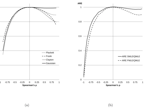
the asymptotic relative efficiency (ARE) of copula based MLE, i.e. the ratio of the asymptotic variance of FMLE to that of QMLE. Joe (2005) shows that ARE depends on the specifica-tion of marginals and copula as well as on the strength of dependence. Moreover, for some asymmetric marginal distributions, e.g., exponential, he finds that ARE for strongly nega-tively dependent data is much larger than for posinega-tively dependent with the same dependence strength. Fig. 1 panel (a) reports the AREs as a function of dependence strength measured by Spearman’s ρ for commonly used copulae, i.e., Gaussian, Clayton, Plackett, Frank. We
report Spearman’sρ in the range from -0.9 to 0.9 as we experienced numerical instability in
the region close to perfect negative or positive dependence for some copulae. Note that the Frank copula can accommodate only positive dependence. These plots confirm that there is a scope for improvement over the QMLE and that the largest gains can be expected in the case of strong negative dependence.
In our simulations we focus on a bivariate DGP with exponential marginals and the Plack-ett copula, which is comprehensive in the sense that it can accommodate the entire range of dependence captured by such measures as Kendall’s τ or Spearman’s ρ. The marginal
dis-tribution parameters (disdis-tribution means µ) are set at 0.5. The copula parameter takes 25
values in the range between 0.001 (Spearman’sρ near -1) and 1,000 (Spearman’s ρnear +1).
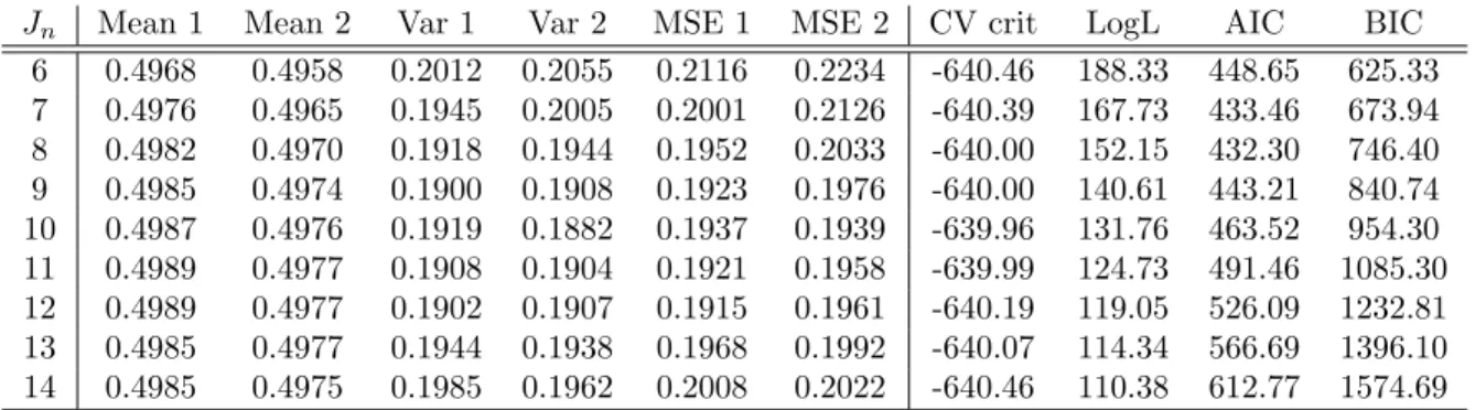
Fig. 1 panel (b) reports the ARE for SMLE and FMLE as a function of Spearman’s ρ
when the data comes from the Plackett copula. The SMLE asymptotic variance is estimated using Eq. (9) for a sample of 200,000 observations, where we use the tensor product sieve with cosine basis functions without the intercept to approximategq. The number of sieve elements
Several observations are interesting in Fig. 1. First, as expected the AREs of both FMLE and SMLE are near one (subject to some estimation noise) in the case of independence, when we expect no gains over QMLE. Second, we observe the lowest ARE, that is the biggest efficiency gains, when Spearman’s ρ approaches -1. This corresponds to extreme negative
dependence and agrees with observations made by Joe (2005). In fact, the ARE of Plack-ett FMLE with copula parameter at 0.001 is 0.035 suggesting a 96.5% improvement over QMLE; the ARE of SMLE for the same strength of dependence is 0.051 suggesting a 94.9% improvement. Third, if we have strong positive dependence then FMLE does not show much efficiency gain over QMLE, which also agrees with Joe (2005). Interestingly, we observe a similar pattern for SMLE.
Joe (2005) provides an explanation for the asymmetry in ARE with respect to ρ. He
observes that the upper and lower limits of dependence correspond to the Fr´echet upper and lower bounds and he derives the constraints on the functional relationship between the two random variables implied by those bounds. Then, efficiency gains of FMLE over QMLE could be obtained only if the parameters of the marginals can be identified from these constraints. It turns out that for the bivariate distribution with exponential marginals under the Fr´echet lower bound the parameters are identified and the ARE goes to zero in the limiting case of strong negative dependence. On the contrary, under the Fr´echet upper bound the parameters of the marginals are not identified and the ARE is approaching one in the limiting case of positive dependence. The simulations summarized in Fig. 1 panel (b) show that similar arguments hold for SMLE.
marginals (not reported here). Interestingly, changing the true values of µ did not affect
the ARE comparisons. This suggests that relative efficiency in estimation of parameters in exponential marginals depends only on the strength of dependence and not on the parameters in the marginals themselves. This isolates the effect of dependence on the ARE and makes exponential marginals particularly attractive for simulation purposes. For non-exponential marginals, the ARE denerally depends on both parameters in the marginals and the depen-dence parameter.
Naturally, the efficiency gains reported in Fig. (1b) using FMLE are higher than those obtained using SMLE. However, in regions close to extreme negative dependence and to independence the gap between the two estimators is diminishing. Also, it is perhaps surprising how close the semiparametric estimator is to a fully parametric one in terms of asymptotic precision. We stress that these results do not depend on the values of parameters in the marginals (other than that they must be identified).
Next we consider the performance of SMLE, FMLE and QMLE for a fixed value of Spear-man’s ρ. We keep exponential marginals and the Plackett copula as the DGP and set the
true parameter value in the marginals at µ1 = µ2 = 0.5 and in the copula at γ = 0.05,
which implies moderate negative dependence with Spearman’s ρ of −0.77. The sample size isN = 1,000 and the number of simulations is R= 1,000.
Table 1 contains the simulation results. We report the mean value of the estimates for each marginal as well as various versions of the variance estimator and the MSE. Under Var, we report sample variance estimates while underAVar, we report estimates of the asymptotic vari-ance obtained using a solution to (9). The number of elements in the Bernstein-Kantorovich
Table 1: Simulated mean and variance for QMLE, SMLE, Plackett copula based FMLE
Parameter µ1 Parameter µ2
FMLE SMLE QMLE FMLE SMLE QMLE Mean 0.5004 0.4987 0.5001 0.4996 0.4976 0.4995
N× Var 0.1720 0.1919 0.2640 0.1740 0.1882 0.2590
N× MSE 0.1721 0.1937 0.2640 0.1741 0.1939 0.2592
N× AVar 0.1580 0.1860 0.2500 0.1580 0.1860 0.2500
Table 2: Optimal number of sieve elements in SMLE
Jn Mean 1 Mean 2 Var 1 Var 2 MSE 1 MSE 2 CV crit LogL AIC BIC
6 0.4968 0.4958 0.2012 0.2055 0.2116 0.2234 -640.46 188.33 448.65 625.33 7 0.4976 0.4965 0.1945 0.2005 0.2001 0.2126 -640.39 167.73 433.46 673.94 8 0.4982 0.4970 0.1918 0.1944 0.1952 0.2033 -640.00 152.15 432.30 746.40 9 0.4985 0.4974 0.1900 0.1908 0.1923 0.1976 -640.00 140.61 443.21 840.74 10 0.4987 0.4976 0.1919 0.1882 0.1937 0.1939 -639.96 131.76 463.52 954.30 11 0.4989 0.4977 0.1908 0.1904 0.1921 0.1958 -639.99 124.73 491.46 1085.30 12 0.4989 0.4977 0.1902 0.1907 0.1915 0.1961 -640.19 119.05 526.09 1232.81 13 0.4985 0.4977 0.1944 0.1938 0.1968 0.1992 -640.07 114.34 566.69 1396.10 14 0.4985 0.4975 0.1985 0.1962 0.2008 0.2022 -640.46 110.38 612.77 1574.69
sieve is 10×10 = 100. This number is picked by cross-validation. A key feature of the table is that SMLE shows substantial improvement over QMLE. The sample variance is close to the asymptotic variance.
Next we look at how the SMLE bias and variance change with the number of sieve el-ements. Table 2 reports means, variances and MSEs for the two estimates as well as the value of log-likelihood and three popular model selection criteria: leave-one-out likelihood cross-validation, AIC and BIC. The value of log-likelihood LogL decreases as sieve
complex-ity grows as expected, while the information criteria AIC and BIC (especially BIC) seem to select an underparameterized model.
4
Application from insurance
We demonstrate the use of SMLE with an insurance application. We have data on 1,500 insurance claims. For each claim, we have the amount of claim payment, or loss, (Y1) and
the amount of claim-related expenses (Y2). The claim-related expenses known as ALAE
(allocated loss adjustment expense) include the insurance company expenses attributable to an individual claim, e.g. the lawyers’ fees and claim investigation expenses. The claim amount variable is censored – there is a dummy variable,d, which is equal to one if a given claim has
surpassed the policy limit and zero if not. For details of the data set, see Frees and Valdez (1998).
The claim amount and ALAE are assumed to be distributed according to the Pareto distribution with parameters (λ1, θ1) and (λ2, θ2), respectively:
Fj(Yj) = 1− λj +Yj λj −θj , j = 1,2. (10)
Interest lies in efficient estimation of the marginal distribution parameters (λ1, θ1, λ2, θ2),
making efficient use of the strong dependence between the claim amount and ALAE. Addi-tional complications arise due to censoring of Y1. The likelihood contributions for censored
observations will not be the same as for the uncensored ones and we need to account for that. Define the marginal pdfs fj(yj), j = 1,2. The QMLE log-likelihood contribution of an
uncensored observation is lnfj(yj), j = 1,2. For a censored observation, the contribution is
claimi is
lQi = (1−di) lnf1(y1i) +diln(1−F1(y1i)) + lnf2(y2i).
Now consider the joint likelihood. Define the joint cdf H(y1, y2) and joint pdf h(y1, y2).
The FMLE contribution of an uncensored observation is lnh(y1, y2) = lnf1(y1) + lnf2(y2) +
lnc(F1(y1), F2(y2)). To derive the contribution of a censored observation we follow Frees and
Valdez (1998) in observing that P rob(Y1 ≥ y1, Y2 ≤ y2) = F2(y2)−H(y1, y2). So the
log-likelihood contribution of a censored observation is f2(y2)−H2(y1, y2), where H2(y1, y2) =
∂H(y1,y2)
∂y2 . But H(y1, y2) = C(F1(y1), F2(y2)) so H2(y1, y2) = C2(F1(y1), F2(y2))f2(y2), where
C2(u1, u2) =
∂C(u1,u2)
∂u2 . Therefore the full log-likelihood contribution for observation i can be
written as
lFi = (1−di)[lnf1(y1) + lnf2(y2) + lnc(F1(y1), F2(y2))]
+di[lnf2(y2) + ln(1−C2(F1(y1), F2(y2)))].
The main difficulty imposed by censoring is that we need to evaluate an additional term involving a copula derivative. For the SMLE, the term is approximated along with lnc.
For the FMLE, the term can be derived analytically for a given copula family or evaluated numerically.
Table 3: QMLE, SMLE, and FMLE for insurance claims and related expenses QML Est. Frank FML Est. G-H FML Est. SML Est. (Rob.St.Er.) (St.Er.) (St.Er.)
λ1 14,443.15 14,562.02 14,040.61 14,631.90 (1,515.09) (1,498.47) (1,351.15) (1,492.36) θ1 1.135 1.115 1.122 1.137 (0.076) (0.073) (0.067) (0.073) λ2 15,133.28 16,708.37 14,223.42 15,421.69 ( 1,744.96) (1,900.49) (1,405.75) (1,663.83) θ2 2.223 2.312 2.119 2.233 (0.183) (0.190) (0.143) (0.172) α - 3.158 -0.791 -(0.171) (0.035) LogL -31,951 -31,778 -31,749 -31,731
the SMLE variance, ˆV, will now be
arg min gq∈AN " N X i=1 (1−di) ( 2 X j=1 ∂lnfj(yji,βˆ) ∂βq + 1 ˆ c(uˆi) ∂ˆc(uˆi) ∂uj ∂Fj(yji,βˆ) ∂βq ! + 1 ˆ c(ˆu1i,uˆ2i) gq(ˆu1i,uˆ2i) ) + N X i=1 di ( ∂lnf2(y2i,βˆ) ∂βq − 1 1−Cˆ2(ˆu1i,uˆ2i) 2 X j=1 ∂Cˆ2(uˆi) ∂uj ∂Fj(yji,βˆ) ∂βq + Z 1 0 gq(s,uˆ2i)ds !)#2 ,
whereβ = (λ1, θ1, λ2, θ2)0, ˆuki =Fk(yki,βˆ) and q= 1, . . . ,4. We will need to evaluate both gq
and its integral over u1.
The three estimators, QMLE, FMLE and SMLE, and their standard errors are given in Table 3. The QMLE is known to be robust in the sense that it is consistent even if independence is a false assumption but to obtain the correct standard errors a “sandwich” formula for variance is needed.
The FMLE estimator is based on a fully specified parametric joint likelihood. We follow Frees and Valdez (1998) and assume the Frank and Gumbel-Hougaard copulas with depen-dence parameter denoted by α, which along with the Pareto marginals completely
param-eterize the model. Consistency of this estimator, sometimes called Pseudo-MLE, relies on correctness of the assumed copula family. If Frank or Gumbel-Hougaard are incorrect copula families then the FMLE will be biased.
The SMLE estimator is robust in the sense that it does not rely on a correctly specified parametric copula family. But it is not as efficient as any fully parametric model. So we should expect SMLE to be close to QMLE in terms of the estimates and to be between FMLE and QMLE in terms of standard errors. To obtain the SMLE, we use the Bernstein-Kantorovich sieve with JN = 10 and to obtain the SMLE standard errors we use the cosine sieve with 9
parameters. The choice of the number of parameters in the Bernstein-Kantorovich sieve is based on cross-validation.
Estimation results support the above intuition. Our FMLE estimates using the Frank and Gumbel-Hougaard copula (which turn out virtually identical to those in Frees and Valdez, 1998) provide evidence of an estimation bias that is not present in QMLE and SMLE, both of which are very close. This supports the robustness (to copula misspecification) argument. The FMLE standard errors are usually smaller than those of QMLE. This indicates higher relative efficiency – a compensation for the lack of robustness. The point we wish to stress is that the SMLE standard errors are smaller than those of QMLE and this gain comes at no robustness cost (but at some computational cost).
5
Concluding Remarks
We have proposed an efficient semiparametric estimator of marginal distribution parameters. This is a sieve maximum likelihood estimator based on a finite-dimensional approximation of the unspecified part of the joint distribution. As such, the estimator inherits the costs and benefits of the multivariate sieve MLE. A major benefit is the increased precision compared to quasi-MLE, permitted by the use of dependence information. Simulations show that potential efficiency gains are huge. The efficiency bound is determined by the dependence strength and we show that our estimator reaches that bound.
The gains come at an increased computational expense. The convergence is slow for the traditional sieves we considered. We found that the Bernstein-Kantorovich polynomial is preferred to other sieves. The running times are greater than the full MLE assuming an “off-the-shelf” parametric copula family but far from being prohibitive (at least for the two dimensional problem we consider). Moreover, simulations reveal a small downward bias in SMLE, which seems to be caused by the sieve approximation error – it decreases as the number of sieve elements increases.
A simple alternative to the proposed method is a fully parametric ML estimation problem. Although simpler computationally, it imposes an assumption on the dependence structure, which, if violated, renders the ML estimates inconsistent. Moreover, robust parametric cop-ulas are often robust because they are redundant. So the proposed estimator seems to offer a unique way of constructing a copula that is robust and generally non-redundant.
Methods to improve computational efficiency of SMLE focus on reducing the effective number of sieve parameters. Such methods involve penalized and restricted estimation and
are particularly appealing for the Bernstein-Kantorovich polynomial where the sparse portions of the sieve parameter space correspond to histogram cells with little or no mass. We leave development of such methods for future work.
References
Ackerberg, D., X. Chen, and J. Hahn(2012): “A Practical Asymptotic Variance Estimator for Two-Step
Semiparametric Estimators,”The Review of Economics and Statistics, 94, 481–498.
Ackerberg, D., X. Chen, J. Hahn, and Z. Liao (2014): “Asymptotic Efficiency of Semiparametric Two-step GMM,”The Review of Economic Studies.
Ai, C. and X. Chen(2003): “Efficient Estimation of Models with Conditional Moment Restrictions
Con-taining Unknown Functions,” Econometrica, 71, 1795–1843.
Amsler, C., A. Prokhorov, and P. Schmidt (2014): “Using copulas to model time dependence in
stochastic frontier models,”Econometric Reviews, 33, 497–522.
Bierens, H. J.(2014): “Consistency and Asymptotic Normality of Sieve ML Estimators under Low-Level Conditions,”Econometric Theory, FirstView, 1–56.
Burda, M. and A. Prokhorov (2014): “Copula based factorization in Bayesian multivariate infinite
mixture models,”Journal of Multivariate Analysis, 127, 200 – 213.
Chen, X.(2007): “Large Sample Sieve Estimation of Semi-Nonparametric Models,” inHandbook of Econo-metrics, ed. by J. J. Heckman and E. E. Leamer, vol. 6, 5549–5632.
Chen, X. and Y. Fan(2006a): “Estimation and model selection of semiparametric copula-based multivariate
——— (2006b): “Estimation of copula-based semiparametric time series models,”Journal of Econometrics, 130, 307–335.
Chen, X., Y. Fan, and V. Tsyrennikov(2006): “Efficient Estimation of Semiparametric Multivariate
Copula Models,”Journal of the American Statistical Association, 101, 1228–1240.
Chen, X. and D. Pouzo(2009): “Efficient estimation of semiparametric conditional moment models with
possibly nonsmooth residuals,”Journal of Econometrics, 152, 46–60.
Frees, E. and E. Valdez(1998): “Understanding relationships using copulas,”North American Actuarial Journal, 2, 1–25.
Ghosal, S.(2001): “Convergence rates for density estimation with Bernstein polynomials,”Annals of Statis-tics, 29, 1264–1280.
Grenander, U.(1981): Abstract Inference, Wiley, New York.
Hafner, C. M. and O. Reznikova (2010): “Efficient estimation of a semiparametric dynamic copula model,”Computational Statistics & Data Analysis, 54, 2609–2627.
Joe, H.(2005): “Asymptotic efficiency of the two-stage estimation method for copula-based models,”Journal of Multivariate Analysis, 94, 401–419.
Kosorok, M.(2008): Introduction to Empirical Processes and Semiparametric Inference, Springer Series in
Statistics, Springer.
Lorentz, G.(1986): Bernstein Polynomials, University of Toronto Press.
Newey, W.(1990): “Semiparametric efficiency bounds,”Journal of Applied Econometrics, 5, 99–135.
Newey, W. K. and J. L. Powell(2003): “Instrumental Variable Estimation of Nonparametric Models,” Econometrica, 71, 1565–1578.
Petrone, S. and L. Wasserman(2002): “Consistency of Bernstein Polynomial Posteriors,”Journal of the Royal Statistical Society. Series B (Statistical Methodology), 64, 79–100.
Prokhorov, A. and P. Schmidt (2009): “Likelihood-based estimation in a panel setting: robustness,
redundancy and validity of copulas,” Journal of Econometrics, 153, 93–104.
Sancetta, A. (2007): “Nonparametric estimation of distributions with given marginals via
Bernstein-Kantorovich polynomials: L1 and pointwise convergence theory,” Journal of Multivariate Analysis, 98, 1376–1390.
Sancetta, A. and S. Satchell (2004): “The Bernstein Copula And Its Applications To Modeling And
Approximations Of Multivariate Distributions,”Econometric Theory, 20, 535–562.
Segers, J., R. v. d. Akker, and B. Werker(2008): “Improving Upon the Marginal Empirical
Distribu-tion FuncDistribu-tions when the Copula is Known,”Tilburg University, Center for Economic Research.
Severini, T. A. and G. Tripathi(2001): “A simplified approach to computing efficiency bounds in semi-parametric models,”Journal of Econometrics, 102, 23–66.
Shen, X.(1997): “On Methods of Sieves and Penalization,”The Annals of Statistics, 25, 2555–2591.
Shen, X. and W. H. Wong(1994): “Convergence Rate of Sieve Estimates,” The Annals of Statistics, 22,
580–615.
Siburg, K. F. and P. A. Stoimenov (2008): “A scalar product for copulas,” Journal of Mathematical Analysis and Applications, 344, 429 – 439.
Sklar, A.(1959): “Fonctions de repartition a n dimensions et leurs marges,” Publications de l’Institut de Statistique de l’Universite de Paris, 8, 229–231.
Stein, C.(1956): “Efficient Nonparametric Testing and Estimation,” Proceedings of Third Berkeley Sympo-sium on Mathematical Statistics and Probability, 1, 187–195.
Tenbusch, A. (1994): “Two-dimensional Bernstein polynomial density estimators,”Metrika, 41, 233–253,
metrika.
Vitale, R.(1975): “A Bernstein polynomial approach to density function estimation,” inStatistical inference and related topics, ed. by M. Puri.
Winkelmann, R. (2012): “Copula bivariate probit models: with an application to medical expenditures,” Health economics, 21, 1444–1455.
Wong, W. H. and T. A. Severini(1991): “On Maximum Likelihood Estimation in Infinite Dimensional Parameter Spaces,”The Annals of Statistics, 19, 603–632.
Zheng, Y.(2011): “Shape restriction of the multi-dimensional Bernstein prior for density functions,” Statis-tics and Probability Letters, 81, 647–651.
6
Appendix
Proof of Theorem 1: Let li(θ) = lnh(yi;θ), l(θ) = N1 P N
i=1li(θ) and 0 < εN = o(N−1/2). We follow
Chen et al. (2006) and consider a continuous pathθ(t) = ˆθ±tεNΠNν∗, t ∈ [0,1], such that θ(0) = ˆθ and
θ(1) = ˆθ±εNΠNν∗.
Under Assumption A2,l(θ) is twice continuously differentiable w.r.t.tand
d l(θ(t)) dt t=τ = 1 N PN i=1 d li(θ(t)) dt t=τ = 1 N PN i=1 d li(θ(τ)) dθ0 [±εNΠNν∗] d2l(θ(t)) dt2 t=τ = 1 N PN i=1 d2l i(θ(τ)) dθ0dθ [±εNΠNν∗,±εNΠNν∗]
By the definition of ˆθ in (4) and the Taylor expansion, 0 ≤ l(ˆθ)−l(ˆθ±εNΠNν∗) =l(θ(0))−l(θ(1)) =− ∂l(∂tθ(t)) t=0− 1 2 ∂2l(θ(t)) ∂t2 t=s, for somes∈[0,1] = ±εN N1 P N i=1 dli( ˆθ) dθ0 [ΠNν∗] +12N1 P N i=1 d2l i(θ(s)) dθ0dθ [±εNΠNν∗,±εNΠNν∗] = ±εN N1 P N i=1 dli( ˆθ) dθ0 [ΠNν∗] +12E d2l i(θ(s)) dθ0dθ [±εNΠNν∗,±εNΠNν∗] +1 2 n 1 N PN i=1 d2l i(θ(s)) dθ0dθ [±εNΠNν∗,±εNΠNν∗]−E d2l i(θ(s)) dθ0dθ [±εNΠNν∗,±εNΠNν∗] o
We follow Chen et al. (2006) and show that
1 N N X i=1 dli(θo) dθ0 [ΠNν ∗−ν∗] =o p(N−1/2) (11)
and that, uniformly overθ(s) in a neighborhood ofθo with||θ(s)−θo||=O(δN),
E d 2l i(θ(s)) dθ0dθ [±εNΠNν ∗,±ε NΠNν∗] =±εNhθˆ−θo, ν∗i ±εNop(N−1/2) (12) and 1 N N X i=1 d2l i(θ(s)) dθ0dθ [±εNΠNν ∗,±ε NΠNν∗]−E d2l i(θ(s)) dθ0dθ [±εNΠNν ∗,±ε NΠNν∗] =εNop(N−1/2) (13)
It will then follow that
0≤l(ˆθ)−l(ˆθ±εNΠNν∗) =±εN N1 P N i=1
dli(θo)
dθ0 [ν∗]±εNhθˆ−θo, ν∗i ±εNop(N−1/2)
And, sinceεN =o(N−1/2)>0, we have
√ Nhθˆ−θo, ν∗i = √1N PN i=1 dli(θo) dθ0 [ν∗]−E dli(θo) dθ0 [ν∗] +oP(1) ⇒ N(0,||ν∗||2), whereEdli(θo) dθ0 [ν∗] = 0 and||ν∗||2=V ardli(θo) dθ0 [ν∗]
of the theorem follows by the Cram´er-Wold device. What remains is to show (11)-(13).
Equation (11) holds by Assumption A4(A), since ||ΠNν∗−ν∗||=o(1). To show (12), note that, under
Assumption A4(B), uniformly overθ(s) in a neighborhood ofθo with||θ(s)−θo||=O(δN),
E d 2l i(θ(s)) dθ0dθ [±εNΠNν ∗,±ε NΠNν∗]≤ hθˆ−θo,±εNΠNν∗i=±εNhθˆ−θo,ΠNν∗i
But, by Assumption A4(A),hθˆ−θo,ΠNν∗−ν∗i=op(N−1/2). Thus,±εNhθˆ−θo,ΠNν∗i=±εNhθˆ−θo, ν∗i ±
εNop(N−1/2). For showing (13), recall that
d2l i(θ(s)) dθ0dθ [±εNΠNν ∗,±ε NΠNν∗] =li(ˆθ±εNΠNν∗)−li(ˆθ)±εN dli(ˆθ) dθ0 [ΠNν ∗]
Now, for someθ(τ) between ˆθand ˆθ±εΠNν∗, writeli(ˆθ±εNΠNν∗)−li(ˆθ) =±εNdlidθ(θ(0τ))[ΠNν∗]. Then, the
left hand side of (13) can be written as
±εN ( 1 N N X i=1 d li(θ(τ)) dθ0 [ΠNν ∗]−Ed li(θ(τ)) dθ0 [ΠNν ∗] ) ±εN ( 1 N N X i=1 d li(ˆθ) dθ0 [ΠNν ∗]−Ed li(ˆθ) dθ0 [ΠNν ∗] ) , which is±εNop(N−1/2).
Proof of Theorem 2: We apply the method of Severini and Tripathi (2001). To make it easier to follow for those who know their method, we use their notation and also specify our equivalents of their objects. For some to > 0 let θ(t) denote a curve from [0, to] into Θ such that θ(0) = θo. The curve we consider is
θ(t) =θo+tν, for anyν∈V. Let ˙θdenote the slope of θ(t) att= 0, i.e. ˙θis tangent to the set Θ atθo. For
our case, ˙θ=ν. LetT(Θ, θo) denote the collection of all such tangents ˙θ0sand let ¯T(Θ, θo) denote the linear
closure ofT(Θ, θo), i.e. the tangent space. In our case, ¯T(Θ, θo) = ¯V.
The objective is to obtain the efficiency bound for estimatingρ(θo) =λ0βo. Stein (1956) is often credited
for being first to suggest that the efficiency bound can be viewed as the upper bound on the asymptotic variance for estimating any one-dimensional subproblem of the original problem. Our one-dimensional subproblem is estimation oft, whose true value is zero. The score for estimatingt= 0 issi= dlidt(θt)
t=0= dlnh(yi;θt) dt t=0=
dlnh(yi;θo)
dθ [ ˙θ]. In our notation, this is just the directional derivative ˙l(θo)[ν] for obsevation i, call it ˙li(θo)[ν].
Then, the Fisher information for estimatingt= 0 is given by||ν||2=Es2
i.
We now look at those one-parameter subproblems that are informative about the feature of interest ρ(θo), specifically, we focus on those curvesθ(t) that satisfy the restrictionρ(θ(t)) =t. This means choosing
among only those ˙θ0sthat satisfy dρ(dtθ(t))
t=0
= 1, or equivalently, only thoseν0s for which ˙ρ(θo)[ν] = 1. A
simplification that applies in our case is that ˙ρ(θo)[ν] = ρ(ν) =λ0νβ. Then, for any consistent estimator ˆt,
AVn√Nρ(θ(ˆt))−ρ(θo) o
=AV(√Nˆt)≥ ||ν||−2. Now to obtain the semiparametric lower bound (SPLB)
for estimating ρ(θo), we look for a ν that maximizes ||ν||−2. As discussed in Severini and Tripathi (2001,
p. 28), the maximization problem can be equivalently written as
SPLB = sup ν∈V¯:ν6=0,λ0ν β=1 ||ν||−2= sup ν∈V¯:ν6=0 ν λ0ν β −2 = sup 06=ν∈V¯ |λ0νβ|2 ||ν||2 = sup ||ν||=1 |λ0νβ|2=||ρ˙(θo)[ν]||2∗,
where||L(ν)||∗ is the norm of a continuous linear functionalL(ν) on the tangent space.
Calculating the norm is usually easier by appealing to the Riesz representation theorem as done in the main text. Basically, instead we look for the representer of the functional. The Riesz representation theorem says that||ρ˙(θo)[ν]||∗=||ν∗||, where ν∗ as defined in (8). Thus, SPLB =||ν∗||2.