Maximum Likelihood Estimation and Uniform Inference with Sporadic Identification Failure

MAXIMUM LIKELIHOOD ESTIMATION AND UNIFORM INFERENCE

WITH SPORADIC IDENTIFICATION FAILURE

By

Donald W. K. Andrews and Xu Cheng

October 2011

COWLES FOUNDATION DISCUSSION PAPER NO. 1824

COWLES FOUNDATION FOR RESEARCH IN ECONOMICS

YALE UNIVERSITY

Box 208281

Maximum Likelihood

Estimation and Uniform Inference

with Sporadic Identi…cation Failure

Donald W. K. Andrews

Cowles Foundation

Yale University

Xu Cheng

Department of Economics

University of Pennsylvania

First Draft: August, 2007

Revised: October 17, 2011

The …rst author gratefully acknowledges the research support of the

National Science Foundation via grant numbers SES-0751517 and

SES-1058376. The authors thank Xiaohong Chen, Sukjin Han, Yuichi

Kitamura, Peter Phillips, Eric Renault, Frank Schorfheide, and Ed

Vytlacil for helpful comments.

Abstract

This paper analyzes the properties of a class of estimators, tests, and con…dence sets (CS’s) when the parameters are not identi…ed in parts of the parameter space. Speci…cally, we consider estimator criterion functions that are sample averages and are smooth functions of a parameter : This includes log likelihood, quasi-log likelihood, and least squares criterion functions.

We determine the asymptotic distributions of estimators under lack of identi…cation and under weak, semi-strong, and strong identi…cation. We determine the asymptotic size (in a uniform sense) of standard t and quasi-likelihood ratio (QLR) tests and CS’s. We provide methods of constructing QLR tests and CS’s that are robust to the strength of identi…cation.

The results are applied to two examples: a nonlinear binary choice model and the smooth transition threshold autoregressive (STAR) model.

Keywords: Asymptotic size, binary choice, con…dence set, estimator, identi…cation, like-lihood, nonlinear models, test, smooth transition threshold autoregression, weak identi-…cation.

1. Introduction

This paper provides a set of maximum likelihood (ML) regularity conditions under which the asymptotic properties of ML estimators and corresponding t and QLR tests and con…dence sets (CS’s) are obtained. The novel feature of the conditions is that they allow the information matrix to be singular in parts of the parameter space. In consequence, the parameter vector is unidenti…ed and weakly identi…ed in some parts of the parameter space, while semi-strongly and strongly identi…ed in other parts. The conditions maintain the usual assumption that the log-likelihood satis…es a stochastic quadratic expansion. The results also apply to quasi-log likelihood and nonlinear least squares procedures.

Compared to standard asymptotic results in the literature for ML estimators, tests, and CS’s, the results given here cover both …xed and drifting sequences of true para-meters. The latter are necessary to treat cases of weak identi…cation and semi-strong identi…cation. In particular, they are necessary to determine the asymptotic sizes of tests and CS’s (in a uniform sense).

This paper is a sequel to Andrews and Cheng (2007a) (AC1). The method of estab-lishing the results outlined above and in the Abstract is to provide a set of su¢ cient conditions for the high-level conditions of AC1 for estimators, tests, and CS’s that are based on smooth sample-average criterion functions. The high-level conditions in AC1 involve the behavior of the estimator criterion function under certain drifting sequences of distributions. In contrast, the assumptions given here are much more primitive. They only involve mixing, smoothness, and moment conditions, plus conditions on the para-meter space.

The paper considers models in which the parameter of interest is of the form = ( ; ; );where is identi…ed if and only if ₆= 0; is not related to the identi…cation of ; and = ( ; ) is always identi…ed. For examples, the nonlinear binary choice model is of the form: Yi = 1(Yi >0)and Yi = h(Xi; ) +Zi0 Ui;where(Yi; Xi; Zi)

is observed and h(; ) is a known function. The STAR model is of the form: Yt =

1+ 2Yt 1+ m(Yt 1; ) +Ut; where Yt is observed and m(; ) is a known function.

In general, the parameters ; ; and may be scalars or vectors. We determine the asymptotic properties of ML estimators, tests, and CS’s under drifting sequences of parameters/distributions. Suppose the true value of the parameter is n = ( n; n; n)

statistics depends on the magnitude of_jj njj:The asymptotic behavior of these statistics

varies across three categories of sequences _f n :n 1g: Category I(a): n= 0 8n 1;

is unidenti…ed; Category I(b): n 6= 0 and n1=2 n !b 2Rd ; is weakly identi…ed;

Category II: _{n !} 0 and n1=2

jj njj ! 1; is semi-strongly identi…ed; and Category

III: _{n! 0 6}= 0; is strongly identi…ed.

For Category I sequences, we obtain the following results: the estimator of is incon-sistent, the estimator of = ( ; )and thet and QLR test statistics have non-standard asymptotic distributions, and the standard tests and CS’s (that employ standard normal or 2 _{critical values) have asymptotic null rejection probabilities and coverage}

probabil-ities that may or may not be correct depending on the model.1 (In many cases, they are not correct). For Category II sequences, estimators and standard tests and CS’s are found to have standard asymptotic properties, but the rate of convergence of the estima-tor of is less thann1=2_{: Speci…cally, the estimators are asymptotically normal and the}

test statistics have asymptotic chi-squared distributions. For Category III sequences, the estimators and standard tests and CS’s have standard asymptotic properties and the estimators converge at rate n1=2_:

We also consider t and QLR tests and CS’s that are robust to the strength of iden-ti…cation. These procedures use di¤erent critical values from the standard ones. First, we consider critical values based on asymptotically least-favorable sequences of distrib-utions. Next, we consider data-dependent critical values that employ an identi…cation-category selection procedure that determines whether is near the value 0 that yields lack of identi…cation of ; and if it is, the critical value is adjusted (in a smooth way) to take account of the lack of identi…cation or weak identi…cation. We show that the ro-bust procedures have correct asymptotic size (in a uniform sense). The data-dependent robust critical values yield more powerful tests than the least favorable critical values.

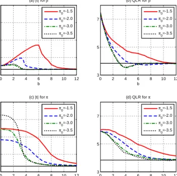
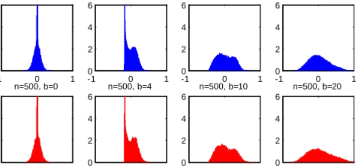
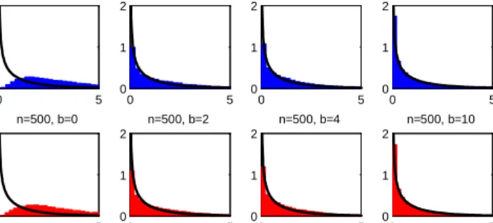
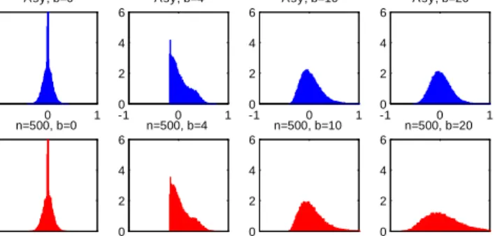
The numerical results for the STAR and nonlinear binary choice models are summa-rized as follows. The asymptotic distributions of the estimators of and are far from the normal distribution under weak identi…cation and lack of identi…cation. The as-ymptotic distributions range from being strongly bimodal, to being close to uniform, to being extremely peaked. The asymptotics provide remarkably accurate approximations to the …nite-sample distributions.

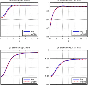
In the STAR model, the standard t and QLR con…dence intervals (CI’s) for have

1_{Here, by “correct”we mean or less for tests and1 or greater for CS’s, where and1 are}

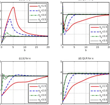
substantial asymptotic size distortions with asymptotic sizes equaling :56 and :72; re-spectively, for nominal :95 CI’s. This is also true for the t and QLR CI’s for ; where the asymptotic sizes are :40 and :84; respectively. Note that the size distortions are noticeably larger for the standardt than QLR CI. In the binary choice model, the stan-dard t and QLR CI’s for have incorrect asymptotic sizes: :68 versus:92; respectively, for nominal :95 CI’s. However, the standard t and QLR CI’s for have small and no size distortion, respectively. In both models, the asymptotic sizes provide very good approximations to the …nite-sample sizes for the cases considered.

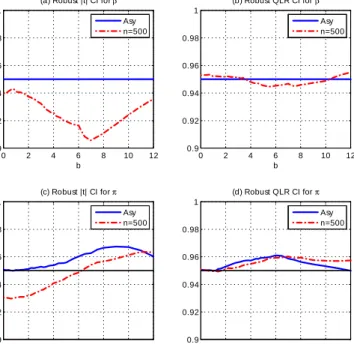
In both models, the robust CI’s have correct asymptotic sizes and …nite-sample sizes that are quite close to the asymptotic size for the QLR CI’s and fairly close for the t

CI’s.

In sum, the numerical results indicate that the asymptotic results of the paper are quite useful in determining the …nite-sample behavior of estimators and standard tests and CI’s under weak identi…cation and lack of identi…cation. They are also quite useful in designing robust tests and CI’s whose …nite-sample size is close to their nominal size. The results of this paper apply when the criterion function satis…es a stochastic quadratic expansion in the parameter : This rules out a number of interesting models that exhibit lack of identi…cation in parts of the parameter space, including regime switching models, mixture models, abrupt transition structural change models, and abrupt transition threshold autoregressive models.2

Now, we brie‡y discuss the literature related to this paper. See AC1 for a more detailed discussion. The following are companion papers to this one: AC1, Andrews and Cheng (2007c) (AC1-SM), and Andrews and Cheng (2008) (AC3). These papers provide related, complementary results to the present paper. AC1 provides results under high-level conditions and analyzes the ARMA(1, 1) model in detail. AC1-SM provides proofs for AC1 and related results. AC3 provides results for estimators and tests based on generalized method of moments (GMM) criterion functions. It provides applications to an endogenous nonlinear regression model and an endogenous binary choice model.

Cheng (2008) provides results for a nonlinear regression model with multiple sources of weak identi…cation, whereas the present paper only considers a single source. However, the present paper applies to a much broader range of models.

Tests of H0 : = 0 versus H1 : 6= 0 are tests in which a nuisance parameter

only appears under the alternative. Such tests have been considered in the literature

starting from Davies (1977). The results of this paper cover tests of this sort, as well as tests for a whole range of linear and nonlinear hypotheses that involve ( ; ; ) and corresponding CS’s.

The weak instrument (IV) literature is closely related to this paper. However, papers in that literature focus on criterion functions that are indexed by parameters that do not determine the strength of identi…cation. In contrast, in this paper, the parameter

; which determines the strength of identi…cation of ; appears as one of parameters in the criterion function. Selected papers from the weak IV literature include Nelson and Startz (1990), Dufour (1997), Staiger and Stock (1997), Stock and Wright (2000), Kleibergen (2002, 2005), Moreira (2003), and Kleibergen and Mavroeidis (2009).

Andrews and Mikusheva (2010) and Qu (2011) consider Lagrange multiplier (LM) tests in a maximum likelihood context where identi…cation may fail, with emphasis on dynamic stochastic general equilibrium models. The results of the present paper apply to t and QLR statistics, but not to LM statistics. The consideration of LM statistics is in progress.

Antoine and Renault (2009, 2010) and Caner (2010) consider GMM estimation with IV’s that lie in the semi-strong category, using our terminology. Nelson and Startz (2007) and Ma and Nelson (2008) analyze models like those considered in this paper. However, they do not provide asymptotic results or robust tests and CS’s of the type given in this paper. Sargan (1983), Phillips (1989), and Choi and Phillips (1992) provide …nite-sample and asymptotic results for linear simultaneous equations models when some parameters are not identi…ed. Phillips and Shi (2011) provide results for a nonlinear regression model with non-stationary regressors in which identi…cation may fail.

The remainder of the paper is organized as follows. Section 2 introduces the smooth sample average extremum estimators, criterion functions, tests, CS’s, and drifting se-quences of distributions considered in the paper. Section 3 states the assumptions em-ployed. Section 4 provides the asymptotic results for the extremum estimators. Section 5 establishes the asymptotic distributions of QLR statistics, determines the asymptotic size of standard QLR CS’s, and introduces robust QLR tests and CS’s, whose asymp-totic size is equal to their nominal size. Section 6 considerst-based CS’s. The nonlinear binary choice model is used as a running example in the previous sections. Section 7 pro-vides results for the smooth transition threshold autoregressive model (STAR) model. Section 8 provides numerical results for the STAR and binary choice models. Appendix A provides proofs of the results given in the paper. Appendix B provides some

mis-cellaneous results. Three Supplemental Appendices to this paper are given in Andrews and Cheng (2007b). Supplemental Appendix C provides additional numerical results for the nonlinear binary choice and STAR models. Supplemental Appendices D and E verify the assumptions for the nonlinear binary choice model and the STAR model, respectively.

All limits below are taken “as n_{! 1}:”Let min(A)and max(A)denote the smallest

and largest eigenvalues, respectively, of a matrixA: All vectors are column vectors. For notational simplicity, we often write (a; b) instead of (a0_{; b}0₎0 _{for vectors a and b: Also,}

for a functionf(c)with c= (a; b) (= (a0_{; b}0₎0_{); we often writef(a; b) instead off(c):Let}

0d denote a d-vector of zeros. Because it arises frequently, we let 0 denote a d -vector

of zeros, where d is the dimension of a parameter : Let R[ 1] = R [ f 1g: Let

R_[p _1]=R[ 1] ::: R[ 1]withpcopies. Let)denote weak convergence of a sequence

of stochastic processes indexed by ₂ for some space :3

2. Estimator and Criterion Function

2.1. Smooth Sample Average Estimators

We consider an extremum estimatorbn that is de…ned by minimizing a sample

cri-terion function of the form

Qn( ) =n 1 n X

i=1

(Wi; ); (2.1)

where _fWi : i ng are the observations and (w; ) is a known function that is twice

continuously di¤erentiable in : This includes ML and LS estimators. The observations fWi : i ng may be i.i.d. or strictly stationary. Formal assumptions are provided in

Section 3 below.

The paper considers the case where is not identi…ed (by the criterion function

Qn( )) at some points in the parameter space. Lack of identi…cation occurs when the Qn( ) is ‡at wrt some sub-vector of : To model this identi…cation problem, is

parti-3_{In the de…nition of weak convergence, we employ the uniform metricdon the spaceE}

vofRv-valued

tioned into three sub-vectors:

= ( ; ; ) = ( ; ); where = ( ; ): (2.2)

The parameter ₂Rd _{is unidenti…ed when = 0 (}

2Rd _{):The parameter = ( ; )}

2

Rd _{is always identi…ed. The parameter}

2 Rd _{does not e¤ect the identi…cation of} :These conditions allow for a wide range of cases, including cases in which reparame-trization is used to convert a model into the framework considered here.

Example 1. This example is the nonlinear binary choice model

Yi = 1(Yi >0) and Yi = h(Xi; ) +Zi0 Ui; (2.3)

where h(Xi; )2 R is known up to the …nite-dimensional parameter 2Rd : Suppose h(x; ) is twice continuously di¤erentiable wrt for any x in the support of Xi and

the …rst- and second-order partial derivatives are denoted by h (x; ) and h (x; );

respectively.

The observed variables are _fWi = (Yi; Xi; Zi) : i = 1; :::; ng: The random variables

f(Xi; Zi; Ui) :i= 1; :::; ngare i.i.d. The distribution of(Xi; Zi)is ;which is an

in…nite-dimensional nuisance parameter. The parameter of interest is = ( ; ; ):Conditional on(Xi; Zi);the distribution function (df) of Ui is L(u): The df L(u) is known and does

not depend on (Xi; Zi): For example, L(u) is the standard normal distribution df in

a probit model and the logistic df in a logit model. We assume that L(u) is twice continuously di¤erentiable and its …rst- and second-order derivatives are denoted by

L0(u) and L00(u); respectively. Suppose L0(u)>0 and 0< L(u)<1₈u₂R:

In this model,

P(Yi = 1jXi; Zi) = P(Ui < h(Xi; ) +Zi0 jXi; Zi) =L(gi( )); where

gi( ) = h(Xi; ) +Zi0 : (2.4)

We estimate = ( ; ; ) by the ML estimator. The sample criterion function is

Qn( ) = n 1 n X

i=1

[YilogL(gi( )) + (1 Yi) log(1 L(gi( ))] (2.5)

standard log-likelihood function so that the estimator minimizes the sample criterion function as in the general set-up of the paper.)

When = 0; gi( ) and Qn( ) do not depend on ;and is not identi…ed.

The true distribution of the observations _fWi : i ng is denoted F for some

parameter ₂ : We let P and E denote probability and expectation under F : The parameter space for the true parameter, referred to as the “true parameter space,”is compact and is of the form:

=_f = ( ; ) : ₂ ; ₂ ( )_g; (2.6)

where is a compact subset of Rd _{and ( )}

8 2 for some compact metric space with a metric that induces weak convergence of the bivariate distributions (Wi; Wi+m) for all i; m 1:4 In unconditional likelihood scenarios, no parameter

appears. In conditional likelihood scenarios, with conditioning variables _fXi : i 1g;

indexes the distribution of _fXi : i 1g: In nonlinear regression models estimated

by least squares, indexes the regression functions and possibly a …nite-dimensional feature of the distribution of the errors, such as its variance, and indexes the remaining characteristics of the distribution of the errors, which may be in…nite dimensional.

By de…nition, the estimatorbn (approximately) minimizes Qn( ) over an

“optimiza-tion parameter space” :5

bn 2 and Qn(bn) = inf

2 Qn( ) +o(n

1

): (2.7)

We assume that the interior of includes the true parameter space (see Assump-tion B1 below). This ensures that the asymptotic distribuAssump-tion of bn is not a¤ected by

boundary constraints for any sequence of true parameters in :The focus of this paper is not on boundary e¤ects.

Without loss of generality (wlog), the optimization parameter space can be written

4_{Thus, the metric satis…es: if !}

0; then (Wi; Wi+m) under converges in distribution to

(Wi; Wi+m)under 0:Note that is a metric space with metricd ( 1; 2) =jj 1 2jj+d ( 1; 2);

where _j= ( j; j)2 forj= 1;2andd is the metric on :

5_Theo(n 1_{)term in (2.7), and in (4.1) and (4.2) below, is a …xed sequence of constants that does}

not depend on the true parameter ₂ and does not depend on in (4.1). Theo(n 1_{)term allows for}

some numerical inaccuracy in practice and circumvents the issue of the existence of parameter values that achieve the in…ma.

as

= _f = ( ; ) : ₂ ( ); _{2 g}; where = _f : ( ; )₂ for some _g and

( ) = _f : ( ; )_{2 g}for ₂ : (2.8)

We allow ( ) to depend on and, hence, need not be a product space between and :For example, this is needed in the STAR model and in the ARMA(1, 1) example in AC1.

Example 1 (cont.). The true parameter space for is

=_{B Z} ; where_B = [ b₁; b₂] R; (2.9)

b₁ 0; b₂ 0; b₁ andb₂ are not both equal to0;_Z ( Rd _{)is compact, and ( R}d ₎

is compact.

The ML estimator of minimizes Qn( ) over 2 : The optimization parameter

space is

=_{B Z} ; where _B= [ b1; b2] R; (2.10)

b1 > b1; b2 > b2; Z ( Rd ) is compact, ( Rd ) is compact, Z 2 int(Z); and

B 2int(_B):

2.2. Con…dence Sets and Tests

We are interested in the e¤ect of lack of identi…cation or weak identi…cation on the extremum estimator bn; on CS’s for various functions r( ) of ; and on tests of null

hypotheses of the formH0 :r( ) =v:

CS’s are obtained by inverting tests. A nominal 1 CS for r( ) is

CSn=fv :Tn(v) cn;1 (v)g; (2.11)

where_Tn(v)is a test statistic, such as the QLR statistic, andcn;1 (v)is a critical value

for testing H0 : r( ) = v: Critical values considered in this paper may depend on the

null value v of r( ) as well as on the data. The coverage probability of a CS forr( ) is

where P ( ) denotes probability when is the true value.

We are interested in the sample size of a CS, which is the smallest …nite-sample coverage probability of the CS over the parameter space. It is approximated by the asymptotic size, which is de…ned as follows:

AsySz = lim inf

n!1 inf2 P (r( )2CSn) = lim infn!1 inf2 P (Tn(r( )) cn;1 (r( ))): (2.13)

For a test, we are interested in the maximum null rejection probability, which is the …nite-sample size of the test. A test’s asymptotic size is an approximation to the latter. The asymptotic size of a test of H0 :r( ) =v is

AsySz= lim sup

n!1

sup

2 :r( )=v

P (_Tn(v)> cn;1 (v)): (2.14)

2.3. Drifting Sequences of Distributions

The uniformity over ₂ for any given sample sizen in (2.13) and (2.14) is crucial for the asymptotic size to be a good approximation to the …nite-sample size. The value of at which the …nite-sample size of a CS or test is attained may vary with the sample size. Thus, to determine the asymptotic size we need to derive the asymptotic distribution of the test statistic_Tn(vn)under sequences of true parameters n = ( n; n)

and vn=r( n) that may depend onn:

As shown in Andrews and Guggenberger (2010) and Andrews, Cheng, and Guggen-berger (2009), the asymptotic size of CS’s and tests are determined by certain drifting sequences of distributions. The following sequences _{f ng}are key:

( ₀) = _{ff n2} :n 1_g: _{n ! 0 2 g}; (2.15) ( ₀;0; b) = n_{f ng 2} ( ₀) : ₀ = 0 and n1=2 _n!b₂Rd_{[ 1]}o; and ( ₀;₁; !0) = f ng 2 ( 0) :n1 =2 jj njj ! 1 and n=jj njj !!0 2Rd ; where 0 = ( 0; 0; 0; 0) and n = ( n; n; n; n):

The sequences in ( ₀;0; b) are in Categories I and II and are sequences for which f ng is close to 0: n ! 0: When jjbjj < 1; f ng is within O(n 1=2) of 0 and the

sequence is in Category I. The sequences in ( ₀;₁; !0)are in Categories II and III and

are more distant from = 0: n1=2

jj njj ! 1:

the true parameters are _f ng 2 ( 0) for any 0 2 ;” “under f ng 2 ( 0;0; b)” to

mean “when the true parameters are _f ng 2 ( 0;0; b) for any 0 2 with 0 = 0and

any b ₂ Rd_{[ 1]};” and “under _f ng 2 ( 0;1; !0)” to mean “when the true parameters

are_{f ng 2} ( ₀;₁; !0) for any 0 2 and any!0 2Rd with jj!0jj= 1:”

3. Assumptions

3.1. Smooth Sample Average Assumptions

This section provides primitive su¢ cient conditions for many of the high-level as-sumptions given in AC1 for the class of sample average criterion functions that are smooth in :Note that the high-level assumptions in AC1 concern limit behavior under drifting sequences of true distributions. In contrast, the assumptions given here concern behavior under …xed true distributions and do not involve the sample sizen:6

In Assumptions S1-S4 below, the true distribution of _fWi : i 1g is F 0: The

conditions in Assumptions S1-S4 are assumed to hold for all ₀ = ( ₀; ₀; 0; 0) 2 :

Let C be a generic …nite positive constant that does not necessarily take the same value when it appears in two di¤erent places. None of the constants that appear in Assumptions S1-S4 depend on 0 2 :

3.1.1. Assumption S1

The …rst assumption is the following.

Assumption S1. Under any _{0 2} ; _fWi : i 1g is a strictly stationary and strong

mixing sequence with mixing coe¢ cients m Cm A for some A > d q=(q d ) and

some q > d 2;or _fWi :i 1g is an i.i.d. sequence and the constantq (that appears

in Assumption S3 below) equals 2 + for some >0:

In Assumption S1, the decay rate of the strong mixing coe¢ cients is used to ob-tain the stochastic equicontinuity of cerob-tain empirical processes using results in Hansen (1996). The WLLN and CLT for strong mixing arrays also hold under this decay rate, see Andrews (1988) and de Jong (1997). In the i.i.d. case, the constantqis smaller than in the strong mixing case, which yields weaker moment restrictions in Assumption S3 below.

Example 1 (cont.). In this example, Assumption S1 holds with q = 2 + for some

>0 because _fWi :i 1g are i.i.d. for each 0 2 :

3.1.2. Assumption S2

The second assumption is as follows.

Assumption S2. (i) For some function (w; )₂R; Qn( ) =n 1Pn_i=1 (Wi; );where (w; )is twice continuously di¤erentiable in on an open set containing ₈w_{2 W}:

(ii) (w; )does not depend on when = 0 ₈w_{2 W}:

(iii) _{8 0 2} with ₀ = 0; E ₀ (Wi; ; ) is uniquely minimized by 0 8 2 :

(iv) _{8 0 2} with _{0 6}= 0; E ₀ (Wi; ) is uniquely minimized by 0:

(v) ( ) is compact _{8 2} ; and and are compact.

(vi) ₈" >0; ₉ > 0 such that dH ( ( 1); ( 2)) < " 8 1; 2 2 with k 1 2k < ;

where dH( ) is the Hausdor¤ metric.

For i.i.d. observations with density f(w; ); the ML estimator is obtained by tak-ing (Wi; ) = logf(Wi; ): For a stationary p-th order Markov process fWi : p+

1 i n_g; we let Wi = (Wi ; :::; Wi p): If the conditional density of Wi given

(W_{i 1}; :::; W_{i p}) is f(w _jW_{i 1}; :::; W_{i p}; ); then the ML estimator is obtained by tak-ing (Wi; ) = logf(WijWi 1; :::; Wi p; ):

Example 1 (cont.). Assumption S2(i) holds in this example with

(Wi; ) =YilogL(gi( )) + (1 Yi) log(1 L(gi( )) (3.16)

by (2.5) and the smoothness conditions on h(Xi; ) and L(u): Assumption S2(ii) holds

becausegi( )does not depend onh(Xi; )when = 0:For brevity, Assumptions S2(iii)

and S2(iv) are veri…ed in Supplemental Appendix D. The argument for Assumption S2(iv) is a standard argument for ML estimators in well-identi…ed scenarios. Assumption S2(v) holds because ( ) =_{B Z}; which does not depend on ; =_{B Z} ;and B; _Z; and are all compact. Assumption S2(vi) holds because ( ) does not depend on :

A class of examples of (w; )functions that satisfy Assumption S2(ii) are functions of the form

x is a sub-vector of w; and a(x; ) and h(x; ) are known functions. In (3.17), (w; ) does not depend on when = 0 because a(x; ) = 0: Examples of a(x; ) include (i) a(x; ) = ; (ii) a(x; ) = exp( ) 1; and (iii) a(x; ) = x0 : Example (i) covers the nonlinear regression example, where is the coe¢ cient of the nonlinear regressor. Example (ii) demonstrates that a(x; ) can be nonlinear in provided a(x; ) = 0 at = 0: Example (iii) covers the weak IV example and the case in which enters the model through a single index. The form in (3.17) does not require a regression model and it allows for complicated structural models by allowing di¤erent functional forms for a(x; ); h(x; ); and (w; ):

Returning now to the general (w; ) case, Assumption S2(vi) holds immediately in cases where ( )does not depend on :When ( )depends on ;the boundary of ( ) is often a continuous linear function of ; as in the STAR model and the ARMA(1,1) model considered in AC1. In such cases, it is simple to verify Assumption S2(vi).

3.1.3. Assumption S3

Let (w; )and (w; ) denote the …rst-order and second-order partial derivatives of (w; ) wrt ; respectively. Let (w; ) and (w; ) denote the …rst-order and

second-order partial derivatives of (w; ) wrt :

We de…ne a matrix B( ) that is used to normalize the second-derivative matrix (w; ) so that its sample average has a nonsingular probability limit. Let

B( ) = " Id 0d d 0d d ( )Id # 2Rd d ; where ( ) = ( if is a scalar jj jj if is a vector : (3.18) We use a di¤erent de…nition of B( ) in the scalar and vector cases because in the scalar case the use of ; rather than _{jj jj};produces noticeably simpler (but equivalent) formulae, but in the vector case _{jj jj} is required.

For ₆= 0; let

B 1( ) (w; ) = y(w; ) and

B 1( ) (w; )B 1( ) = y (w; ) + 1( )"(w; ); (3.19) where y (w; )is symmetric and y(w; ); y (w; );and "(w; ) satisfy Assumption S3 below. The re-scaling matrix B 1_{( )in (3.19) is used to deal with the singularity issue}

that arises when = 0:In particular, the covariance matrix of (Wi; )is singular when

= 0 and close to singular when is close to 0. In contrast, the re-scaled quantity

y_{(Wi; )has a covariance matrix that is not close to being singular even when is close}

to 0. Similarly,E

0 (Wi; )is singular when = 0and close to singular when is close

to0: Re-scaling of (Wi; )yields a quantity y (Wi; )whose expectation is not close

to singular even when is close to 0 plus another term "(Wi; ) that is asymptotically

negligible.

Below we illustrate the form of y(w; ); y (w; );and "(w; )in Example 1 and for (w; )functions as in (3.17), see Section 3.1.4.

Next, de…ne Vy( 1; 2; 0) = 1 X m= 1 Cov ₀( y(Wi; 1); y(Wi+m; 2)); (3.20)

which does not depend on i because the observations are stationary under Assumption S1. Under Assumptions S1 and S3(iii) below, Vy₍

1; 2; 0) exists by a standard strong

mixing inequality.

The form of Assumption S3 di¤ers depending on whether is a scalar or vector. We state Assumption S3 for the scalar case …rst because it is simpler.

Assumption S3 (scalar ). (i) E ₀"(Wi; 0) = 0 and j 0j 1jjE 0"(Wi; 0; )jj

C_jj 0jj 8 0 2 with 0<j 0j< for some >0:

(ii) For all > 0 and some functions M1(w) : W ! R+ and M2(w) : W ! R+;

jj (w; 1) (w; 2)jj+jj y (w; 1) y (w; 2)jj M1(w) andjj y(w; 1) y(w; 2)jj

+_jj"(w; 1) "(w; 2)jj M2(w) ; 8 1; 2 2 with jj 1 2jj ; 8w2 W:

(iii)E ₀sup _{2 fj} (Wi; )j1+ +jj (Wi; )jj1+ +jj y (Wi; )jj1+ +M1(Wi)+jj y(Wi; )jjq

+_jj"(Wi; )jjq+M2(Wi)qg C for some >08 0 2 ;whereq is as in Assumption S1.

(iv) min(E 0 (Wi; 0; )) > 0 8 2 when 0 = 0 and E 0

y _(W

i; 0) is positive

de…nite ₈ 0 2 :

(v) Vy( 0; 0; 0)is positive de…nite 8 0 2 :

In Assumption S3(iii), the last three terms have bounded qth moments in order to establish the stochastic equicontinuity of empirical processes based on y(Wi; ) and "(Wi; ) using Lemma 9.4 in Appendix A.

In Assumptions S1-S3, Assumptions S2(ii), S2(iii), S3(i), S3(iii), S3(iv) and S3(v) are related to the weak identi…cation problem. Assumption S2(ii) implies that the sample

criterion function is ‡at in when = 0;as in Assumption A of AC1. Assumption S2(iii) di¤ers from a standard condition in the sense that the population criterion function is not uniquely minimized by the true value when 0 = 0: The Lipschitz condition

in Assumption S3(i) typically holds because the partial derivative of E

0"(Wi; 0; )

wrt is approximately proportional to _{jj 0jj} when _{jj 0jj} is close to 0: Because parts of

B 1_{( )diverge as converges to 0, the moment conditions for} y_(W

i; )and y (Wi; )in

Assumption S3(iii) are stronger than standard moment conditions on the …rst-order and second-order derivatives. These conditions hold in typical examples, see below, because the partial derivative of (w; ) wrt is small when is close to 0 under Assumption S2(ii). Hence, the rhs moments are uniformly bounded even after the scaling byB 1_{( ):}

In Assumptions S3(iv) and S3(v),E ₀ y (Wi; 0)andVy( 0; 0; 0)typically are positive

de…nite due to the re-scaling in (3.19).

Under Assumptions S1-S3, the criterion functionQn( )has probability limitQ( ; ) = E (Wi; ) under any sequence of parameters n ! :

Example 1 (cont.). In this example, y(Wi; ); y (Wi; ); and "(w; ) are de…ned

as follows. For notational simplicity, let Li( ); L0i( ); and L00( ) abbreviate L(gi( )); L0_(g

i( ));and L00(gi( ));respectively. Let

d ;i( ) = (h(Xi; ); Zi0)0; di( ) = (h(Xi; ); Zi0; h (Xi; )0)0; and Di( ) = 2 6 4 0 01 d h (Xi; )0 0d 1 0d d 0d d h (Xi; ) 0d d h (Xi; ) 3 7 5: (3.21)

The …rst-and second-order partial derivatives of (Wi; ) wrt to and are

(Wi; ) = w1;i( )(Yi Li( ))d ;i( ); (Wi; ) = w1;i( )(Yi Li( ))B( )di( ); (Wi; ) = [w12;i( )(Yi Li( ))2+w2;i( )(Yi Li( ))]d ;i( )d ;i( )0; (Wi; ) = [w21;i( )(Yi Li( ))2+w2;i( )(Yi Li( ))]B( )di( )di( )0B( ) +w1;i( )(Yi Li( ))Di( ); where w1;i( ) = L0 i( ) Li( )(1 Li( )) and w2;i( ) = L00 i( ) Li( )(1 Li( )): (3.22)

The re-scaled partial derivatives in (3.19) take the form y_(W i; ) = w1;i( )(Yi Li( ))di( ); y _(W i; ) = [w12;i( )(Yi Li( ))2+w2;i( )(Yi Li( ))]di( )di( )0; and "(w; ) = w1;i( )(Yi Li( )) 2 6 4 0 01 d h (Xi; )0 0d 1 0d d 0d d h (Xi; ) 0d d h (Xi; ) 3 7 5: (3.23)

To verify Assumption S3(i), note that E ₀(YijXi; Zi) = P 0(Yi = 1jXi; Zi) = Li( 0)

by (2.4). Hence, E ₀(Yi Li( 0)jXi; Zi) = 0 implies E 0"(Wi; 0) = 0 by the law of

iterated expectations (LIE).

Let L0_i = sup _{2 j}L0_i( )_jand L00_i = sup _{2 j}L00_i( )_j:

A mean-value expansion of Li( 0; )wrt around 0 yields

Li( 0; ) Li( 0) = L0i( 0;e)

@gi( 0;e)

@ 0 ( 0)

= L0_i( ₀;_e)h (Xi; 0;e)0 0( 0); (3.24)

where _e is between and 0: To verify the second part of Assumption S3(i), we have

jjE ₀(w1;i( 0; )[Yi Li( 0; )]h (Xi; ))jj = _jjE ₀(w1;i( 0; )[Li( 0) Li( 0; )]h (Xi; ))jj j 0j jj 0jjE 0(w1;iL 0 ih 2 ;i) Cj 0j jj 0jj; (3.25)

for someC <₁;where the equality holds by LIE, the …rst inequality holds using (3.24), and the second inequality holds by the Cauchy-Schwarz inequality and the moment conditions in (3.32).

Similarly, we have

jjE ₀(w1;i( 0; )[Yi Li( 0; )]h (Xi; ))jj Cj 0j jj 0jj (3.26)

for some C < ₁: By (3.23), (3.25), and (3.26), the second part of Assumption S3(i) holds.

When is a vector, i.e., d > 1; we reparameterize as (_{jj jj}; !); where ! =

=_{jj jj} if ₆= 0 and by de…nition ! = 1d =jj1d jj with 1d = (1; :::;1) 2 Rd if = 0:

Correspondingly, is reparameterized as + = (_{jj jj}; !; ; ): Let + = _f + : + = (_{jj jj}; =_{jj jj}; ; ); _{2 g}:

This new parameterization is needed when is a vector because y(w; ); y (w; );

and "(w; ) typically involve =_{jj jj} due to the re-scaling in (3.19) and =_{jj jj} is not continuous in for ₂ :In consequence, the Lipschitz conditions in Assumptions S3(ii) and S3(iii) (scalar ) can not be veri…ed when is a vector. The new parameterization treats _{jj jj} and ! = =_{jj jj} as separate variables. In Assumption S3 (vector ) below, some Lipschitz conditions are speci…ed in terms of + = (_{jj jj}; !; ; ):

In Assumption S3 (vector ), both the original parameterization with and the alternative parameterization with + are employed for convenience. Note that only con-ditions related to y(w; ); y (w; );and"(w; )require the alternative parameterization with +:

Assumption S3 (vector ). (i) E ₀"(Wi; 0) = 0 and jj 0jj 1jjE 0"(Wi;

+₎

jj

C(_jj 0jj +jj! !0jj) 8 + = (jj 0jj; !; 0; ) and 8 0 2 with 0 < jj 0jj <

for some >0:

(ii) For all > 0 and some functions M1(w) : W ! R+ and M2(w) : W ! R+;

jj (w; 1) (w; 2)jj + jj y (w; +1) y (w; + 2)jj M1(w) and jj (w; 1) (w; 2)jj+jj y(w; +1) y(w; + 2)jj+jj"(w; + 1) "(w; + 2)jj M2(w) ; 8 1; 2 2 with _jj 1 2jj ; 8 +1; + 2 2 + with jj + 1 + 2jj ; 8w2 W:

(iii) Assumptions S3(iii)-(iv) (scalar ) hold with the de…nitions of M1(w) and M2(w)

replaced by those given above.

Assumption S3(i) (vector ) typically holds because the partial derivatives ofE ₀"(Wi;

+_{) wrt and ! are approximately proportional to}

jj 0jj:

3.1.4. Forms of y(w; ); y (w; ); and "(w; )

Now, we illustrate the forms of y(w; ); y (w; ); and "(w; ) when (w; ) be-longs to the class speci…ed in (3.17) and show that Assumption S3(i) holds in this case. For simplicity, we assume a(x; ) and h(x; ) are both scalars and no parame-ter appears. Let 0_{( ) and} 00_{( ) abbreviate the …rst- and second-order derivatives of}

(w; a(x; )h(x; )) wrt a(x; )h(x; ): Let a (x; ); a (x; ); h (x; ); h (x; ) de-note the …rst- and second-order partial derivatives of a(x; ) and h(x; ) wrt and :

The …rst and second order partial derivatives of (w; ) wrt to and are

(w; ) = 0( )a (x; )h(x; ); (w; ) = 0( )a(x; )h (x; );

(w; ) = 00( )a (x; )a (x; )0h2(x; ) + 0( )a (x; )h(x; );

(w; ) = 00( )a(x; )h(x; )a (x; )h (x; )0 + 0( )a (x; )h (x; )0; and (w; ) = 00( )a2(x; )h (x; )h (x; )0+ 0( )a(x; )h (x; ): (3.27) In this case, we have

y_{(w; ) =} 0_{( )a}y_{(x; );} y _{(w; ) =} 00_{( )a}y_{(x; )a}y_{(x; )}0_{; where} ay(x; ) = (a (x; )0h(x; );a(x; ) ( ) h (x; ) 0₎0 _and "(w; ) = 0( ) " a (x; )h(x; ) a (x; )h (x; )0 h (x; )a (x; )0 a(x; ) ( ) h (x; ) # : (3.28)

Note that 1a(x; ) is continuous at = 0 in the scalar case. In particular, lim _!0 1a(x; ) =a (x;0)by a mean-value expansion becausea(x;0) = 0 anda(x; )

is continuously di¤erentiable in :In the vector case, lim _!0; =jj jj!!0jj jj

1_{a(x; ) =}

a (x;0)!0:

When "(w; ) takes the form in (3.28), Assumption S3 below implies Assumption S3(i). In Assumption S3 (i), Xi is a sub-vector of Wi that takes the place of x in w:

Assumption S3 . (i) Xi is a vector of weakly exogenous variables such that

E ₀( 0_(W

i; a(Xi; 0)h(Xi; 0))jXi) = 0 a.s. 8 0 2 :

(ii)E ₀sup_{jj jj< ; 2 j} 00_(W

i; a(Xi; )h(Xi; ))j (jjh(Xi; )jj+jjh (Xi; )jj) (jh(Xi; )j+

jjh (Xi; )jj+jjh (Xi; )jj) sup_{jj jj}< jja (Xi; )jj (jja (Xi; )jj+jja (Xi; )jj) C

for some C <₁ and >0 _{8 0 2} :

Several of the derivatives in Assumption S3 (ii) are constants in many examples, which makes the moment condition in Assumption S3 (ii) less restrictive than it may appear. For example, when a(Xi; ) = ; a (Xi; ) = 1 and a (Xi; ) = 0:

Lemma 3.1. Suppose (w; ) belongs to the class in (3.17), where a(x; ) ₂ R and

h(x; ) ₂ R are twice di¤erentiable wrt and ; respectively, and no parameter appears. Then, "(w; ) takes the form in (3.28) and Assumption S3(i) is implied by Assumption S3 in both the scalar and vector cases.

Comment. When (w; ) belongs to the class in (3.17) and a parameter appears, the form of "(w; ) is the same as in (3.28) but with zeros in the rows and columns that correspond to : In this case, Assumption S3(i) is still implied by Assumption S3 provided 0_{( ) and} 00_{( ) in Assumption S3 are adjusted to include ; evaluated at}

0:

See Appendix B for details.

3.1.5. Assumption S4

Next, we state an assumption that controls how the mean E _{0 ;i}( ) changes as the true 0 changes, where 0 = ( 0; 0; 0; 0): De…ne the d d -matrix of partial

derivatives of the average population moment function wrt the true value, 0; to be

K( ; ₀) = @

@ 0₀E 0 (Wi; ): (3.29)

The domain of the function K( ; ₀) is 0; where = f 2 : jj jj < g and 0 =f a = (a ; ; ; )2 : = ( ; ; ; )2 with jj jj< and a 2[0;1]g for some

>0:7

Assumption S4. (i)K( ; ₀)exists ₈( ; ₀)₂ 0:

(ii) K( ; ) is continuous in ( ; ) at ( ; ) = (( ₀; ); ₀) uniformly over ₂ 8 0 2 with 0 = 0; where 0 is a sub-vector of 0:

Assumption S4 is not restrictive in most applications.8

For simplicity, K( ₀; ; ₀) is abbreviated asK( ; ₀):

Example 1 (cont.). It is shown in Supplemental Appendix D that Assumption S4

holds with K( ; ₀) = K( ₀; ; ₀) = E ₀ L 02 i ( 0) Li( 0)(1 Li( 0)) h(Xi; 0)d ;i( ) (3.30) for ₀ = ( 0; 0):

7_{The constant >0is as in Assumption B2(iii) stated below. The set}

0is not empty by Assumption

B2(ii).

8_{Assumptions S1 and S4 imply Assumption C5 of AC1. A set of primitive su¢ cient conditions for}

Assumption C5 of AC1 is given in Appendix A of AC1-SM. These conditions also are su¢ cient for Assumption S4.

3.2. Parameter Space Assumptions

Next, we specify conditions on the parameter spaces and :

De…ne = _{f 2} : _{jj jj} < _g; where is the true parameter space for ; see (2.6). The optimization parameter space satis…es:

Assumption B1. (i)int( ) :

(ii) For some >0; _{f 2}Rd :_{jj jj}< _{g Z}0 _{for some non-empty open}

set _Z0 Rd and as in (2.8). (iii) is compact.

Because the optimization parameter space is user selected, Assumptions B1(ii)-(iii) can be made to hold by the choice of :

The true parameter space satis…es:

Assumption B2. (i) is compact and (2.6) holds.

(ii)₈ >0; ₉ = ( ; ; ; )₂ with 0<_{jj jj} < :

(iii) ₈ = ( ; ; ; ) ₂ with 0 < _{jj jj} < for some > 0; _a = (a ; ; ; ) ₂ 8a₂[0;1]:

Assumption B2(ii) guarantees that is not empty and that there are elements of whose values are non-zero but are arbitrarily close to0;which is the region of the true parameter space where near lack of identi…cation occurs. Assumption B2(iii) ensures that is compatible with the existence of partial derivatives of certain expectations wrt the true parameter around = 0; which arise in (3.29) and Assumption S4.

Example 1 (cont.). Let = ( ; );where is the distribution of(Xi; Zi);and 2 ;

where is a compact metric space with some metric that induces weak convergence. The parameter space for the true value of is

=_f = ( ; ) : ₂ ; ₂ ( )_g; (3.31)

where ( ) _{8 2} :

The parameter space ( ); which must be speci…ed precisely to obtain the uni-form asymptotic results, is de…ned as follows. For notational simplicity, let hi =

sup _{2 j}h(Xi; )j; h ;i= sup ₂ jjh (Xi; )jj; h ;i = sup ₂ jjh (Xi; )jj; w1;i= sup ₂

For any 0 2 ; the true parameter space for is ( 0) = f 0 2 : E 0(h 4q i +h 4q ;i+h 4q ;i+jjZijj4q+w41q;i+w 2+ 2;i ) C jjw1;i( 1) w1;i( 2)jj M1(Wi)jj 1 2jj; jjw2;i( 1) w2;i( 2)jj M2(Wi)jj 1 2jj; jjh (Xi; 1) h (Xi; 2)jj Mh(Wi)jj 1 2jj;

8 1; 2 2 for some functions M1(Wi); M2(Wi); Mh(Wi); E 0(M1(Wi) 4q=3_+M 2(Wi)4=3+Mh(Wi)4q=3) C; E ₀sup 2 j logLi( )j1+ +jlog(1 Li( ))j1+ C; P ₀(a0(h(Xi; 1); h(Xi; 2); Zi) = 0)<1; 8 1; 2 2 with 1 6= 2; 8a2Rd +2

with a₆= 0; E ₀di( )di( )0)is positive de…nite 8 2 g (3.32)

for some C <₁; where di( ) = (h(Xi; ); Zi0; h (Xi; )0)0:9

3.3. Key Quantities

Now, we de…ne some of the key quantities that arise in the asymptotic distribution of the estimatorbn and the test statistics considered. Let S = [Id : 0d d ]denote the d d selector matrix that selects out of : De…ne

( 1; 2; 0) = S Vy(( 0; 1);( 0; 2); 0)S0;

H( ; ₀) = E ₀ (Wi; 0; );

J( ₀) = E ₀ y (Wi; 0); and

V( ₀) = Vy( 0; 0; 0): (3.33)

Example 1 (cont.). The key quantities that determine the asymptotic behavior of the ML estimator in the binary choice model are as follows. The probability limit of the criterion function Qn( ) when the true value is 0 2 is

Q( ; ₀) = E ₀ (Wi; ) = E ₀E ₀( (Wi; )_jXi; Zi)

= E ₀[Li( 0) logLi( ) + (1 Li( 0)) log(1 Li( ))]: (3.34)

9_{In (3.32), the expectationE}

0( )only depends on 0:Because 0 shows up in some other

By calculations given in Section 13.1 of Supplemental Appendix D, we have ( 1; 2; 0) = E 0 L02 i ( 0) Li( 0)(1 Li( 0)) d ;i( 1)d ;i( 2)0; H( ; ₀) = E 0 L02 i ( 0) Li( 0)(1 Li( 0)) d ;i( )d ;i( )0; and J( ₀) = V( ₀) =E ₀ L 02 i ( 0) Li( 0)(1 Li( 0)) di( 0)di( 0)0: (3.35)

3.4. Quadratic Approximations

Here we specify certain quadratic approximations to Qn( ) and related results that

hold under Assumptions S1-S4, B1, and B2. These results help to explain the form of the asymptotic distributions that arise in the results stated below.

(i) Under _f ng 2 ( 0;0; b) (de…ned in (2.15) above), the sample criterion function

Qn( ) (= Qn( ; ))has a quadratic expansion in around the point 0;n = (0; n) for

given for the form:

Qn( ; ) = Qn( 0;n; ) +D Qn( 0;n; )0( 0;n) +

1

2( 0;n)

0_D

Qn( 0;n; )( 0;n) +Rn( ; ); (3.36)

where D Qn( 0;n; ) and D Qn( 0;n; ) denote the vector and matrix of …rst and

second partial derivatives of Qn( ; ) with respect to ;respectively, evaluated at =

0;n; and Rn( ; ) is a remainder term that is small uniformly in 2 for close to

0;n:10

(ii) Under _f ng 2 ( 0;1; !0); the sample criterion function Qn( ) has a quadratic

expansion in around the true value n of the form:

Qn( ) =Qn( n) +DQn( n)0( n) +

1

2( n)D

2_Q

n( n)( n) +Rn( ); (3.37)

where DQn( n) and D2Qn( n)denote the vector and matrix of …rst and second partial

derivatives ofQn( ) with respect to ; respectively, evaluated at = n; and Rn( ) is a

10_{The precise conditions that the remainderR}

n( ; )satis…es are speci…ed in Assumption C1 of AC1.

The quadratic approximation result (i) and results (ii)-(iv) that follow are established in the proof of Theorem 4.1 given in Appendix A.

remainder term that is small for close to n:11

(iii) Under _f ng 2 ( 0;0; b); the recentered and rescaled …rst derivative of Qn( )

wrt satis…es an empirical process CLT:

Gn( ) ) G( ; 0); where Gn( ) = n 1=2 n X i=1 ;i( 0;n; ) E n ;i( 0;n; ) (3.38)

andG( ; ₀)is a mean zero Gaussian process indexed by ₂ with bounded continuous sample paths and covariance kernel ( 1; 2; 0) for 1; 2 2 :

(iv) Under _{f ng 2} ( ₀;₁; !0); the rescaled …rst and second derivatives of Qn( )

satisfy n1=2B 1( _n)DQn( n)!dG ( 0) N(0d ; V( 0)) (3.39) and Jn =B 1( n)D 2 Qn( n)B 1( n)!p J( 0)2R d d 8 0 2 : (3.40)

3.5. Assumptions C6 and C7

In this section, we state assumptions that concern the minimum of the limit of the normalized criterion function after has been concentrated out.12

De…ne a “weighted non-central chi-square” process _f ( ; ₀; b) : _{2 g} and a non-stochastic function _f ( ; ₀; !0) : 2 gby ( ; ₀; b) = 1 2(G( ; 0) +K( ; 0)b) 0_H 1_{( ;} 0) (G( ; 0) +K( ; 0)b) and ( ; ₀; !0) = 1 2! 0 0K( ; 0)0H 1_{( ;} 0)K( ; 0)!0: (3.41)

The process ( ; ₀; b) is the limit under _{f ng 2} ( ₀;0; b) for _jjb_jj < ₁; de…ned in (2.15), and the function ( ; ₀; !0) is the limit under f ng 2 ( 0;0; b) for jjbjj = 1:

Under Assumptions S1-S4, _f ( ; ₀; b) : _{2 g} has bounded continuous sample paths a.s.

To obtain the asymptotic distribution of _bn when n=O(n 1=2)via the continuous

mapping theorem, we use the following assumption.

11_{The precise conditions that the remainderR}

n( ) satis…es are speci…ed in Assumption D2 of AC1.

12_{Assumptions C6 and C7 are the same as in AC1, which is why the numbering starts at C6, rather}

Assumption C6. Each sample path of the stochastic process _f ( ; ₀; b) : _{2 g} in some set A( ₀; b) with P ₀(A( ₀; b)) = 1 is minimized over at a unique point (which may depend on the sample path), denoted ( ₀; b); _{8 0 2} with 0 = 0; 8b with

jjb_jj<₁:

In Assumption C6, ( ₀; b) is random.

Next, we give a primitive su¢ cient condition for Assumption C6 for the case where is a scalar parameter. Let (w; ) = ( (w; )0_{; (w; )}0₎0_{:When = 0; (w; )does}

not depend on by Assumption S2(ii) and is denoted by (w; ): When d = 1 and

0 = 0;de…ne (Wi; 0; 1; 2) = ( (Wi; 0; 1); (Wi; 0; 2); (Wi; 0)0)0 and G( 1; 2; 0) = 1 X m= 1 Cov ₀( (Wi; 0; 1; 2); (Wi+m; 0; 1; 2)): (3.42)

Assumption C6y_{. (i)d = 1 (i.e., is a scalar).}

(ii) G( 1; 2; 0) is positive de…nite 8 1; 2 2 with 1 6= 2;8 0 2 with 0 = 0:

Lemma 3.2. Assumptions S1-S3 and C6y imply Assumption C6:

Example 1 (cont.). For this example, Assumption C6y _{is veri…ed in Supplemental}

Appendix D with the covariance matrix in Assumption C6y(ii) equal to

G( 1; 2; 0) = E 0

L02_(Z0

i 0)

L(Z0

i 0)(1 L(Zi0 0))

hZ;i( 1; 2)hZ;i( 1; 2)0; where

hZ;i( 1; 2) = (h(Xi; 1); h(Xi; 2); Zi0)0: (3.43)

The following assumption is used in the proof of consistency of _bn for the case where

the true parameter _n satis…es _n!0 and n1=2

jj njj ! 1:

Assumption C7. The non-stochastic function ( ; ₀; !0) is uniquely minimized over

2 at 0 8 0 2 with 0 = 0:

In Assumption C7, 0 is non-random. Assumption C7 can be veri…ed using the

Cauchy-Schwarz inequality or a matrix version of it, see Tripathi (1999), whenK( ; ₀) and H( ; ₀)take proper forms, as in our examples.

Example 1 (cont.). Assumption C7 is veri…ed in this example as follows. By (2.4) and (3.35), when 0 = 0; H( ; ₀) = E ₀ L 02_(Z0 i 0) L(Z0 i 0)(1 L(Zi0 0)) d ;i( )d ;i( )0: (3.44) By (2.4) and (3.30), when ₀ = 0; K( ; ₀) = E ₀ L 02_(Z0 i 0) L(Z0 i 0)(1 L(Zi0 0)) h(Xi; 0)d ;i( ): (3.45) Hence, when 0 = 0; K( ; ₀)0H 1( ; ₀)K( ; ₀) E ₀ L 02_(Z0 i 0) L(Z0 i 0)(1 L(Zi0 0)) h2(Xi; 0) (3.46)

by the matrix Cauchy-Schwarz inequality in Tripathi (1999). The “ ” holds as an equality if and only if h(Xi; 0)a+d ;i( )0b = 0 with probability 1 for somea 2R and b ₂Rd +1 _{with (a; b}0_{)6= 0:The “ ”holds as an equality uniquely at =}

0 because for

any ₆= 0; P 0(c

0_(h(X

i; 0); h(Xi; ); Zi0)0 = 0)<1for any c6= 0 by (3.32).

4. Estimation Results

This section provides the asymptotic results of the paper for the extremum estimator

bn:The results are given under the drifting sequences of distributions de…ned in Section

2.3. De…ne a concentrated extremum estimator b_n( ) (₂ ( )) of for given ₂ by

Qn(bn( ); ) = inf

2 ( )

Qn( ; ) +o(n 1): (4.1)

Let Qc_n( ) denote the concentrated sample criterion function Qn(bn( ); ): De…ne

an extremum estimator bn (2 ) by Qc_n(_bn) = inf

2 Q

c

n( ) +o(n 1): (4.2)

We assume that the extremum estimator bn in (2.7) can be written as bn =

(b_n(_bn);bn): Note that if (4.1) and (4.2) hold and bn = (bn(bn);bn); then (2.7)

For n= ( n; n; n; n)2 ;letQ0;n =Qn( 0;n; ); where 0;n= (0; n):Note that Q0;n does not depend on by Assumption S2(ii).

De…ne the Gaussian process _f ( ; ₀; b) : _{2 g} by

( ; ₀; b) = H 1( ; ₀)(G( ; ₀) +K( ; ₀)b) (b;0d ); (4.3)

where (b;0d ) 2 Rd : Note that, by (3.41) and (4.3), ( ; 0; b) = (1=2)( ( ; 0; b) +

(b;0d ))0H( ; 0)( ( ; 0; b) + (b;0d )): Let

( ₀; b) = arg min

2

( ; ₀; b): (4.4)

Theorem 4.1. Suppose Assumptions S1-S4, B1, B2, and C6 hold. Under _{f ng 2}

( ₀;0; b) with _jjb_jj<₁; (a) n 1=2₍b n n) bn ! !d ( ( ₀; b); ₀; b) ( ₀; b) ! ; and (b) n Qn(bn) Q0;n !dinf 2 ( ; 0; b):

Comments. 1. The results of Theorem 4.1 and Theorem 4.2 below are like those of Theorems 5.1 and 5.2 of AC1. However, Theorems 4.1 and Theorem 4.2 are obtained under assumptions that are much more primitive and easier to verify, though less general, than the results in AC1. In particular, Assumptions S1-S4 impose conditions for …xed parameters, not conditions on the behavior of random variables under sequences of parameters. In addition, explicit formulae for the components of the asymptotic results are provided here based on the sample average form of Qn( ) that is considered.

2. De…ne the Gaussian process _f ( ; ₀; b) : _{2 g} by

( ; ₀; b) = S ( ; ₀; b) +b; (4.5)

where S = [Id : 0d d ] is the d d selector matrix that selects out of : The

asymptotic distribution ofn1=2b

n(without centering at n) under ( 0;0; b)withjjbjj<

1 is given by ( ( ₀; b); ₀; b):

3. Assumption C6 is not needed for Theorem 4.1(b). Let

Theorem 4.2. Suppose Assumptions S1-S3, B1, B2, and C7 hold. Under _f ng 2

( ₀;₁; !0);

(a) n1=2B( _n)(bn n)!d J 1( 0)G ( 0) N(0d ; J 1( 0)V( 0)J 1( 0)); and

(b) n(Qn(bn) Qn( n))!d 1₂G ( 0)0J 1( 0)G ( 0):

5. QLR Con…dence Sets

In this section, we consider CS’s based on the quasi-likelihood ratio (QLR) statistic. We establish (i) the asymptotic distribution of the QLR statistic under the drifting sequences of distributions de…ned in Section 2.3, (ii) the asymptotic size of standard QLR CS’s, which often are size-distorted, and (iii) the correct asymptotic size of robust QLR CS’s, which are designed to be robust to the strength of identi…cation. The proofs of the results given here rely on results given in Appendix A and AC1.

5.1. De…nition of the QLR Test Statistic

We consider CS’s for a function r( ) (₂ Rdr_{) of obtained by inverting QLR tests.}

The function r( ) is assumed to be smooth and to be of the form

r( ) = " r1( ) r2( ) # ; (5.7)

where r1( )2Rdr1; dr1 0 is the number of restrictions on ; r2( ) 2R

dr_{2; d}

r2 0 is

the number of restrictions on ; and dr =dr1 +dr2:

For v ₂ r( ); we de…ne a restricted estimator en(v) of subject to the restriction

that r( ) =v: By de…nition,

e_n(v)₂ ; r(en(v)) =v; and Qn(en(v)) = inf

2 :r( )=vQn( ) +o(n

1

): (5.8)

The QLR test statistic for testing H0 :r( ) =v is

QLRn(v) = 2n(Qn(en(v)) Qn(bn))=bsn; (5.9)

where _bsn is a random real-valued scaling factor that is employed in some cases to yield

See Assumptions RQ2 and RQ3 below.

Let cn;1 (v) denote a nominal level 1 critical value to be used with the QLR

test statistic. It may be stochastic or non-stochastic. The usual choice, based on the asymptotic distribution of the QLR statistic under standard regularity conditions, is the 1 quantile of the 2

dr distribution, which we denote by

2

dr;1 :

Given a critical value cn;1 (v); the nominal level 1 QLR CS forr( ) is

CS_r;nQLR =_fv ₂r( ) :QLRn(v) cn;1 (v)g: (5.10)

5.2. QLR Assumptions

Ifr( )includes restrictions on ;i.e.,dr2 >0;then not all values 2 are consistent

with the restriction r2( ) = v2: For v2 2 r2( ); the set of values that are consistent

with r2( ) =v2 is denoted by

r(v2) = f 2 :r2( ) =v2 for some = ( ; )2 g: (5.11)

If dr2 = 0; then by de…nition r(v2) = 8v2 2r2( ):

We assume r( ) satis…es:

Assumption RQ1. (i)r( ) is continuously di¤erentiable on :

(ii)r ( ) (= (@=@ 0)r( )) is full row rank dr 8 2 :

(iii) r( ) satis…es (5.7).

(iv) dH( r(v2); r(v0;2))!0as v2 !v0;2 8v0;2 2r2( ):

(v)Q( ; ; ₀)is continuous in at 0 uniformly over 2 (i.e.,sup 2 jQ( ; ; 0)

Q( ₀; ; ₀)_{j !}0 as _! 0)8 0 2 with 0 = 0:

(vi) Q( ; ₀) is continuous in at 0 8 0 2 with 0 6= 0:

In Assumption RQ1(iv), dH denotes the Hausdor¤ distance. In Assumptions RQ1(iv)

and (v), Q( ; ₀) = E ₀ (Wi; ):

Assumptions RQ1(i) and RQ1(ii) are standard and are not restrictive. Assumption RQ1(iii) rules out the case where any single restriction depends on both and : This is restrictive. But, in some cases, a reparametrization can be used to obtain results for such restrictions, see AC1 for details. Assumption RQ1(iv) is not very restrictive and is easy to verify in most cases. Assumptions RQ1(v) and RQ1(vi) are not restrictive.

Even under strong identi…cation, it is known that the QLR statistic has an asymp-totic 2_dr null distribution only under additional assumptions to those used for Wald and Lagrange multiplier (LM) statistics. The following two assumptions are needed.

Assumption RQ2. (i) V( ₀) = s( ₀)J( ₀) for some non-random scalar constant

s( ₀) _{8 0 2} ; or (ii) V( ₀) and J( ₀) are block diagonal (possibly after reordering their rows and columns), the restrictions r( ) only involve parameters that correspond to one block of V( ₀) and J( ₀); call them V11( 0) and J11( 0); and for this block

V11( 0) =s( 0)J11( 0)for some non-random scalar constant s( 0) 8 0 2 :

Assumption RQ3. The scalar statistic_bsnsatis…esbsn!p s( 0)underf ng 2 ( 0;0; b)

and under _f ng 2 ( 0;1; !0):

For example, Assumptions RQ2(i) and RQ3 hold withs( ₀) =_bsn = 1 for a correctly speci…ed log-likelihood criterion function. For a homoskedastic nonlinear regression model, Assumptions RQ2(i) and RQ3 hold with s( ₀) equal to the error variance 2

and _bsn equal to a consistent estimator of 2; such as the sample variance based on the

residuals.

5.3. QLR Asymptotic Distributions

To obtain the asymptotic size of QLR CS’s, we need to determine the limits of the coverage probabilities of the QLR CS’s under all sequences _f ng 2 ( 0;0; b) and

f ng 2 ( 0;1; !0) when the null hypotheses are true. That is, we need to know

these limits when v = vn = r( n) for n = ( n; n) 8n 1: To obtain these coverage

probabilities, we …rst determine the asymptotic null distributions of the QLR statistic under these sequences.

In the results below, we use the following notational simpli…cations:

QLRn =QLRn(vn)and en =en(vn); wherevn=r( n) and n = ( n; n):13 (5.12)

For notational simplicity, let r;0 = r(v0;2);where v0;2 =r2( 0) and 0 = ( 0; 0)2

:That is, r;0 is the set of values that are compatible with the restrictions on when 0 is the true parameter value.

13_{As a consequence of these de…nitions, the asymptotic results given below for the statisticsQLR}

nand

en under f ng 2 ( 0;0; b)and underf ng 2 ( 0;1; !0)are results that hold when the restrictions

Next, we introduce the limit under _f ng 2 ( 0;0; b) with jjbjj < 1 of the

re-stricted concentrated criterion function after suitable normalization. De…ne the process f r( ; 0; b) : 2 g by r( ; 0; b) = ( ; 0; b) + 1 2 ( ; 0; b) 0_{P ( ;} 0)0H( ; 0)P ( ; 0) ( ; 0; b); where P ( ; ₀) = H 1( ; ₀)r1; ( 0)0 r1; ( 0)H 1( ; 0)r1; ( 0)0 1 r1; ( 0); (5.13)

r1; ( ) = (@=@ 0)r1( )2Rdr1 d ;and ( ; 0; b)is de…ned in (4.3). Thed d -matrix

P ( ; ₀) is an oblique projection matrix that projects onto the space spanned by the rows of r1; ( 0):

The following Theorem shows that the QLR statistic converges in distribution to

QLR( 0)=s( 0) under f ng 2 ( 0;1; !0); where QLR( 0) is de…ned by

QLR( 0) = G ( 0)0J 1( 0)P ( 0)0J( 0)P ( 0)J 1( 0)G ( 0);

P ( ₀) = J 1( ₀)r ( 0)0 r ( 0)J 1( 0)r ( 0)0 1

r ( 0); (5.14)

r ( 0) = (@=@ 0)r( 0); and J( 0) and G ( 0) are de…ned in (3.33) and (3.39),

respec-tively. Thed d -matrix P ( ₀)is an oblique projection matrix that projects onto the space spanned by the rows of r ( 0):

Theorem 5.1. Suppose Assumptions S1-S4, B1, B2, RQ1, and RQ3 hold. (a)Under _{f ng 2} ( ₀;0; b) with _jjb_jj<₁;

QLRn !d2(inf 2 r;0 r( ; 0; b) inf 2 ( ; 0; b))=s( 0):

(b)Under_{f ng 2} ( ₀;₁; !0); QLRn!d QLR( 0)=s( 0)provided Assumption C7also

holds.

Comment. By Theorem 5.1(b) and some calculations, when Assumptions RQ2 also

holds,

QLRn!d QLR( 0)=s( 0) 2

dr: (5.15)

5.4. Asymptotic Size of Standard QLR Con…dence Sets

Here we establish the asymptotic size of a standard nominal1 CS forr( ) ₂Rdr

obtained by inverting the QLR statistic, de…ned in (5.10), using the 2

dr critical value.

Let h= (b; ₀); H =_fh= (b; ₀) :_jjb_jj<₁; _{0 2} with 0 = 0g; and QLR(h) = 2( inf 2 r;0 r ( ; ₀; b) inf 2 ( ; 0; b))=s( 0) (5.16)

for _jjb_jj <₁: Note that QLR(h) is the asymptotic distribution of QLRn under f ng 2

( ₀;0; b) for _jjb_jj < ₁ by Theorem 5.1(a). Let cQLR;1 (h) denote the 1 quantile

of QLR(h) for h₂H:

The asymptotic size results given below use the following df continuity assumption, which typically is not restrictive.

Assumption RQ4. The df of QLR(h) is continuous at (i) 2

dr;1 and (ii) suph2H

cQLR;1 (h); 8h2H:

Theorem 5.2. Suppose Assumptions S1-S4, B1, B2, C7, RQ1-RQ3, and RQ4(i)hold. Then, the asymptotic size of the standard nominal 1 QLR CS is

AsySz = min_finf

h2HP(QLR(h)

2

dr;1 ); 1 g:

Comment. Depending on the distribution of _fQLR(h) : h ₂ H_g; the standard QLR CS has asymptotic size equal to 1 or less than1 : Often, it is less than1 and the standard QLR CS is size distorted.

5.5. Robust QLR Con…dence Sets

In this section, we construct two QLR CS’s that have correct asymptotic size. These CS’s arerobust to the strength of identi…cation. We construct CS’s forr( )by inverting a robust QLR test that combines the QLR test statistic with a robust critical value that di¤ers from the standard strong-identi…cation critical value, which is a 2

dr quantile.

The …rst robust CS uses the least favorable (LF) critical value. The second robust CS is introduced in AC1. It is more sophisticated and uses a data-dependent critical value. It is called a type 2 robust CS. It is smaller than the LF robust CS under strong identi…cation.

5.5.1. Least Favorable Critical Value

The LF critical value is

cLF_QLR;1 = max_fsup

h2H

cQLR;1 (h); 2dr;1 g: (5.17)

The LF critical value can be improved (i.e., made smaller) by exploiting the knowl-edge of the null hypothesis value of r( ): For instance, if the null hypothesis speci…es the value of to be 3; then the supremum in (5.17) does not need to be taken over all h ₂ H; only over the h values for which = 3: We call such a critical value a null-imposed (NI) LF critical value. Using a NI-LF critical value increases the computational burden because a di¤erent critical value is employed for each null hypothesis value.14;15

When part of is unknown underH0 but can be consistently estimated, then a

plug-in LF (or plug-in NI-LF) critical value can be used that has correct size asymptotically and is smaller than the LF (or NI-LF) critical value. The plug-in critical value replaces elements of with consistent estimators in the formulae in (5.17) and the supremum overH is reduced to a supremum over the resulting subset ofH; denotedHbn;for which

the consistent estimators appear in each vector :16

5.5.2. Type 2 Robust Critical Value

Next, we improve on the LF critical value by employing an identi…cation category selection (ICS) procedure that uses the data to determine whetherb is …nite.17

By Theorem 4.2, the asymptotic covariance matrix ofbn under strong identi…cation

is ( ₀) =J 1₍

0)0V( 0)J 1( 0):Let bn=Jbn1(bn)Vbn(bn)Jbn1(bn)denote an estimator

14_{To be precise, let H(v) = fh = (b;}

0) 2 H : jjbjj < 1; r( 0) = vg; where 0 = ( 0; 0): By

de…nition,H(v)is the subset isH that is consistent with the null hypothesis H0:r( 0) =v;where 0

denotes the true value. The NI-LF critical value, denoted cLF

QLR;1 (v);is de…ned by replacing H by

H(v)in (5.17) when the null hypothesis value isr( 0) =v:Note thatvtakes values in the setVr=fv0:

r( 0) =v0 for someh= (b; 0)2Hg:

15_{Whenr( ) = and the null hypothesis imposes that =v; the parameter b can be imposed to}

equal n1=2v:In this case, H(v) =Hn(v) =fh= (b; 0)2H :b=n1=2vg:The asymptotic size results

given below for NI-LF CI’s and NI robust CI’s hold in this case.

16_{For example, if is consistently estimated byb}

n;thenH is replaced byHbn=fh= (b; )2H : =

( ;b_n; ; )_g:If a plug-in NI-LF critical value is employed,H(v)is replaced byH(v)_\Hbn;whereH(v)

is de…ned in a footnote above. Note that the parameterb is not consistently estimable, so it cannot be replaced by a consistent estimator.

17_{When the null hypothesis speci…es the value of ; it is not necesary to use an ICS procedure.}

of ( ₀); where Jbn( ) and Vbn( ) are estimators with probability limits J( ; 0) and

V( ; ₀);respectively, under n! 0 and J( 0) = J( 0; 0)and V( 0) =V( 0; 0):For

brevity, we state the formal consistency Assumptions V1 and V2 concerning Jnb( ) and

b

Vn( ) in Appendix B.

Example 1 (cont.) In this example, we estimate J( ₀) = V( ₀) by Jbn(bn) =Vbn(bn);

where b Jn( ) =Vbn( ) =n 1 n X i=1 L02 i ( ) Li( )(1 Li( )) di( )di( )0: (5.18)

The ICS procedure chooses between the identi…cation categories _IC0 :jjbjj<1and

IC1 :jjbjj=1:The statistic used for identi…cation-category selection is

An= nb 0 nb 1 ;nbn=d 1=2 ; (5.19)

where b ;n is the upper leftd d block of bn: We use An to assess the strength of

identi…cation.

Now, we de…ne the type 2 robust critical value, which provides a continuous transition from a weak-identi…cation critical value to a strong-identi…cation critical value using a transition function s(x): Let s(x) be a continuous function on [0;₁) that satis…es: (i) 0 s(x) 1;(ii)s(x)is non-increasing inx;(iii)s(0) = 1;and (iv)s(x)_!0asx_{! 1}:

Examples of transition functions include (i) s(x) = exp( c x) for somec > 0 and (ii)

s(x) = (1 +c x) 1 _{for somec >0:}18 _{For example, in the binary choice example, we use}

the function s(x) = exp( x=2):

The type 2 robust critical value is

bcQLR;1 ;n = (

cB if An

cS + [cB cS] s(An ) if An> ; where

cB = cLFQLR;1 + 1; cS = 2dr;1 + 2; (5.20)

and 1 0 and 2 0 are asymptotic size-correction factors that are de…ned below.

Here, “B” denotes Big, and “S” denotes Small. When An ; bcQLR;1 ;n equals the

LF critical value cLF_QLR;1 plus a size-correction factor 1: When An > ; bcQLR;1 ;n

18_IfcLF

QLR;1 =1;one should takes(x)to equal0forxsu¢ ciently large and de…ne1 0in (5.20)

to equal0:Then, the critical value_bcQLR;1 ;nis in…nite ifAn is small and is …nite ifAn is su¢ ciently

is a convex combination of cLF_QLR;1 + 1 and d2r;1 + 2; where 2 is another

size-correction factor and the weight given to the standard critical value 2_dr;1 increases with the strength of identi…cation, as measured byAn :

The ICS statistic An satis…es An !d A(h) under f ng 2 ( 0;0; b) with jjbjj < 1;

where A(h) is de…ned by

A(h) = ( ; ₀; b)0 1( ; ₀) ( ; ₀; b)=d 1=2; (5.21) where abbreviates ( ₀; b); ( ; ₀; b)is de…ned in (4.5), and ( ; ₀)is the upper left (1,1) element of ( ₀; ; ₀)for ( ; ₀) =J 1( ; ₀)V( ; ₀)J 1( ; ₀):19;20;21

Under _{n 2} ( ₀;0; b) with _jjb_jj<₁; the asymptotic null rejection probability of a test based on the statisticQLRn and the robust critical value bcQLR;1 ;n is equal to

N RP( 1; 2;h) =P(QLR(h)> cB &A(h) ) +P(QLR(h)> cA(h) &A(h)> )

=P(QLR(h)> cB) +P(QLR(h)2(cA(h); cB] & A(h)> ); where

cA(h) = cS+ (cB cS) s(A(h) ): (5.22)

The constants 1 and 2 are chosen such thatN RP( 1; 2;h) 8h2H:In

par-ticular, we de…ne 1 = suph2H1 1(h); where 1(h) 0 solves N RP( 1(h);0;h) =

(or 1(h) = 0 if N RP(0;0;h)< ); H1 =f(b; 0) : (b; 0)2 H & jjbjj jjbmaxjj+Dg;

bmaxis de…ned such thatcQLR;1 (h)is maximized overh2Hathmax= (bmax; max)2H

for some max 2 ; and D is a non-negative constant, such as 1: We de…ne 2 =

su