Xavier University
Exhibit
Mathematics
Undergraduate
2016
The Optimization behind Support Vector
Machines and an Application in Handwriting
Recognition
Caitlin Snyder
Xavier University - Cincinnati, [email protected]
Follow this and additional works at:
http://www.exhibit.xavier.edu/undergrad_mathematics
Part of the
Computer Sciences Commons, and the
Mathematics Commons
This Article is brought to you for free and open access by the Undergraduate at Exhibit. It has been accepted for inclusion in Mathematics by an authorized administrator of Exhibit. For more information, please [email protected].
Recommended Citation
Snyder, Caitlin, "The Optimization behind Support Vector Machines and an Application in Handwriting Recognition" (2016). Mathematics.Paper 4.
The Optimization behind Support Vector
Machines and an Application in Handwriting
Recognition
Caitlin Snyder
April 29, 2016
Abstract
Support Vector Machines(SVMs) are a unique tool for classification of data and are used for solving real world problems such as image classifica-tion and text analysis. This project explores the underlying mathematics optimization problem behind the algorithm in a Support Vector Machine. The original minimization problem is described and an equivalent maxi-mization formulation is derived. Various two and three dimensional exam-ples are given to illustrate how the optimization gives a useable result with both linearly and nonlinearly separable data. Finally, this tool is applied in a handwriting character recognition problem. Popular SVM kernels are explored and their respective accuracy percentages in identifying between characters are compared.
1
Introduction
My motivation to learn about Support Vector Machines stemmed from my REU over the summer. We used SVMs to classify Implicit Association Test takers as cheaters or non-cheaters. Implicit Association Tests are utilized to determine if a person has a bias by measuring reaction times when classifying objects (terms or pictures). A person is able to cheat the test by slowing down their reaction times if they are aware of how bias is measured. A problem exists with simply looking at reaction times and classifying the slow times as cheaters. People with naturally slower reaction times or those who may become distracted during the test may be incorrectly classified as cheaters. The SVM is useful in this type of classification because it is able to determine a connection between cheaters that a human eye may not see. It is also helpful with Implicit Association Tests because the test taker is asked to classify up to 200 objects and can analyze the times much quicker. For this project, I explore the underlying optimization method and study examples in 2 and 3 dimensions of small data sets. I also focus on a different application for SVMs: handwriting and letter recognition.
2
Background - What is a SVM?
Support Vector Machines are a machine learning tool utlilized for data classifica-tion and regression. The implementaclassifica-tion of a Support Vector Machine requires two sets of data: training and testing. The training data is classified into the correct categories by the user. From this data, a model is produced through an optimization problem. This model creates a hyperplane which linearly separates the testing data set into the correct classifications.
3
Example in 2D with 20 data points
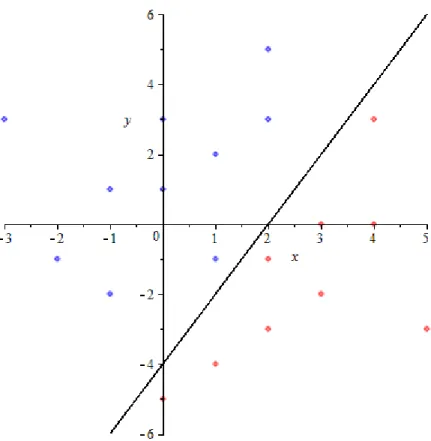
Support Vector Machines are usually applied to large data sets in high dimen-sions that are hard, or impossible, to separate by hand. In order to understand how a SVM works, it is helpful to look at an example that can be solved rela-tively easily. In this example there are 20 data points:
x1= (4,3), y1= 1 x2= (3,0), y2= 1 x3= (4,0), y3= 1 x4= (2,−1), y4= 1 x5= (3,−2), y5= 1 x6= (2,−3), y6= 1 x7= (1,−4), y7= 1 x8= (0,−5), y8= 1 x9= (2,−5), y9= 1 x10= (5,−3), y10= 1 x11= (−3,3), y11=−1 x12= (0,3), y12=−1 x13= (0,1), y13=−1 x14= (1,2), y14=−1 x15= (2,3), y15=−1 x16= (−1,1), y16=−1 x17= (2,5), y17=−1 x18= (−2,−1), y18=−1 x19= (−1,−2), y19=−1 x20= (1,−1), y20=−1
Thexi variables denote the data point and theyi variables denote which cate-gory each point is classified as. It is common practice to use 1 and -1 to denote the two different categories. In a problem existing in the nth dimension, the xi variables will be vectors of lengthn while theyi variables will always be 1 or -1. Each entry in thexi vector will be assigned information. For example, say we would like to separate data points that represent people that make over $75,000 a year and those that make less than $75,000 a year. Theyi would be 1 for those who make over $75,000 and -1 would represent those who make less than $75,000. Each entry in thexivector would represent different information like age, gender, career, location, etc.
In order to separate the data points, a hyperplane is used (discussed in the next section). The data in this example can be separated using the line:
2x−y−4 = 0
Figure 1: Example in 2D with 20 points
4
Hyperplane
The equation for the hyperplane created by the SVM is based on a training data set. The training data set is composed of labeled vectors that are of the form (xi, yi) such thatxiis theithvector in the data set andyi is the label as-sociated withxi. The labelyiindicates which category theithvector belongs in. The equation of a hyperplane comes from a linear discriminant function
f(x) =wTx+b (1)
where b is the bias term and w is the weight vector. When f(x) = 0 we call this the seperating hyperplane because it divides the space into two classes dependent upon the sign of the discriminant function. In two dimensions,w=< w1, w2>andx=< x, y >will result in a line,f(x) =w1x+w2y+b.
Consider the example in Section 3,w=<2,−1>,x=< x, y >, andb=−4. wTx+b= 0 =⇒ 2x−y−4 = 0
This line is the separating hyperplane for this data set. Consider the vectors x1=<4,3>andx11=<−3,3>from this example. Evaluating the
discrimi-nant function with each results in:
f(x1) =f(<4,3>) =<2,−1>T<4,3>−4 = 1
f(x2) =f(<−3,3>) =<2,−1>T<−3,3>−4 =−1
The different signs off(x1) andf(x11) indicate thatx1andx11belong to two
different class, which is true sincef(x1) has the label y1 = 1 and f(x11) has
the labely11=−1.
5
What is the Optimal Hyperplane?
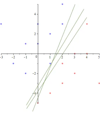
The goal of a SVM is to create a model that produces a hyperplane which will linearly separate a data set into specific categories. However, there are many different hyperplanes that could achieve this goal for any given data set. Figure 2 below illustrates this point for the example described above. The question emerges: which hyperplane is optimal?
5.1
Margin
The margin of a hyperplane [1] is defined as mD(w) = 1
2wˆ
T(x+−x
−) (2)
where wˆ is the unit vector of the weight vector, w, andx+,x−, the support
vectors, are the points closest to the hyperplane. From the definition of the hyperplane,
f(x+) =wTx++b f(x−) =wTx−+b.
Assume thatx+,x− are equidistant from the hyperplane, such thatf(x+) =a
andf(x−) =−afor some postive, constanta. [1]
Set a = 1 by manipulating the data points by a fixed number until this is true (Note: this doesn’t really change the margin, just the units). Subtracting f(x+) andf(x−) leads to the equation:
Figure 2: Many Possible Separating Hyperplanes
buta= 1 so,
wT(x+−x−) = 2
Dividing this equation by||w||results in: w ||w|| T (x+−x−) = 2 ||w||.
By the definition of unit vector and dividing by 2, this simplifies to: 1 2wˆ T(x+−x −) = 1 ||w||. (3)
From the definition of margin (2) and (3) , mD(w) = 1
||w||. (4)
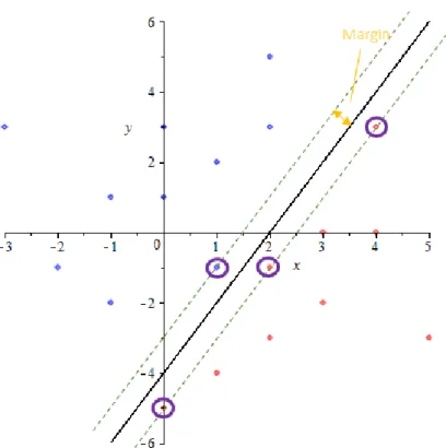
Figure 3 below illustrates the margin of the separating hyperplane in the exam-ple described in Section 3. The circled points indicate the support vectors.
Figure 3: Margin and Support Vectors
5.2
Why do we care about the margin?
The goal of a SVM is to create a model that produces a hyperplane which will linearly separate data into specific categories. An ideal hyperplane would not only separate the training set of vectors but would correctly classify other data sets. The optimal hyperplane will have a maximized margin. If the distance between the closest vector and the hyperplane is large there is a smaller chance that a vector will be incorrectly classified.
Maximizing equation (4) is equivalent to the optimization problem: minimize w,b 1 2||w|| 2 subject to yi(wTxi+b)≥1. (5)
The contraints force every vector to be classified into the correct category (in-dicated byyi’s). Using the definition of the discriminant function (1), we could re-write the constraints to be
The constraints requires the label of the vectors and evaluation of the discrim-inant function to have the same sign. Consider the hyperplane example in Section 4 where f(x) =< 2,−1 >T x−4. Suppose the vector x1 =<4,3 >
has label y1 = −1 and is incorrectly classified. Evaluating the discriminant fuction results inf(x) = f(< 4,3 >) = 1. This violates the constraints since yif(x) =−1 1. Thus incorrectly classifying vectors is impossible with the given constraints.
5.3
Soft-Margin SVM
The requirement of correct classification for every training vector in the opti-mization problem descibed above defines it as a Hard-Margin SVM. The goal of a SVM is to create a model that will linearly separate data sets into correct classifications. The model is created from the training vectors but a good model could be used on other similar data sets. For example, earlier we described a problem where we wanted to classify a person based on if they earning more or less than $75,000. We would input a data set where each person was classified as earning more or less than $75,000 and the SVM would output a model of a hy-perplane to separate them. We already know if each person from the input data set made more or less than $75,000 so it wouldn’t make sense to use this model to classify one of them. The model is actually useful for people that we have no idea how much they make. In this case, we don’t really care if all of the training vectors are classified as correct, just enough to make the model accurate enough. The more commonly used Support Vector Machine, called a Soft-Margin SVM, allows for error in the classification of the training data. It is defined as follows:
minimize w,b 1 2||w|| 2+CX i=1 ξi subject to yi(wTxi+b)≥1−ξi.
where ξi’s are slack variables that allow an example to be in the margin(1 ≥ ξi≥0) or misclassified (ξi≥1) and the constantCsets the relative importance of maximizing the margin and minimizing the amount of slack.
The Soft-Margin SVM requires a balance between not misclassifying too many training vectors and maximizing the margin. The constant C which controls this balance, is one of the user inputs the SVM requires.
6
Kernels
So far we have been looking at data sets that are linearly separable. However, most data sets are not linearly separable in their given form. How does the SVM handle this?
6.1
Kernel Example
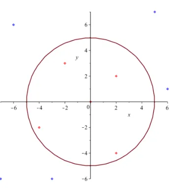
Consider the data points: x1= (0,0), y1= 1 x2= (2,2), y2= 1 x3= (2,−4), y3= 1 x4= (−4,−2), y4= 1 x5= (−2,3), y5= 1 x6= (6,1), y6=−1 x7= (5,7), y7=−1 x8= (−6,6), y8=−1 x9= (−7,−6), y9=−1 x10= (−3,−6), y10=−1
Performing the same optimization process we used for the example in Section 3 will result in a linearly separating hyperplane, a line in this case. As shown in Figure 4, these data points are separated by a circle and a line would incorrecly classify many points.
Figure 4: Kernel Example
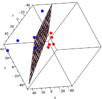
A solution to this problem emerges if we map these 2-dimensional data points into 3 dimensions. Consider the function
φ:R27→R3 φ(x1, x2) = (x21, x 2 2, √ 2x1x2)
x01=φ(0,0) = (0,0,0) x02=φ(2,2) = (4,4,4√2) x03=φ(2,−4) = (4,9,−6 √ 2) x04=φ(−4,−2) = (4,16,−8 √ 2) x05=φ(−2,3) = (16,4,8 √ 2) x06=φ(6,1) = (9,36,18√2) x07=φ(5,7) = (25,49,35√2) x08=φ(−6,6) = (36,1,6 √ 2) x09=φ(−7,−6) = (36,36,−36 √ 2) x010=φ(−3,−6) = (49,36,42 √ 2) Note: The labels,yis, do not change.
The figure below illustrates the points and the hyperplane that separates them.
Figure 5: Projected Points in 3D
6.2
Dual Formulation
For the optimization problem in (5) the Lagrangian is defined as [2]:
L(w, b, α) = 1 2||w|| 2− m X i=1 αi(yi(xTiw+b)−1) (6)
where theαisare the Lagrange multipliers.
The general form of the optimization problem can be defined as: minimize
x f(x)
subject to ci(x)≥0 for alli∈[n].
(7) Theorem 1(Karush-Kuhn-Tucker (KKT) for Differentiable Convex Problems). A solution to the optimization problem (7) with convex, differentiable f, ci is given byx¯, if there exists someα¯∈Rn withα
i≥0 for alli∈[n]such that the following conditions are satisfied:
∂xL(¯x,α¯) =∂xf(¯x) + n X
i=1 ¯
αi∂xci(¯x) = 0 (Saddle Point inx¯) (8) ∂αiL(¯x,α¯) =ci(¯x)≤0 (Saddle Point inα¯) (9)
n X
i=1 ¯
αici(¯x) = 0 (Vanishing KKT-Gap). (10)
From Theorem 1, the Lagrangian (6) must be maximized with respect toαi and minimized with respect tow andb. In other words, from (8)
∂
∂bL(w, b, α) = 0, ∂
∂wL(w, b, α) = 0.
Taking the partial of the Lagrangian with respect tobleads to: ∂ ∂bL(w, b,α) = ∂ ∂b 1 2||w|| 2− n X i=1 (αiyixTiw+αiyib−αi) ! = n X i=1 αiyi Similarly, taking the partial of the Lagrangian with respect towleads to:
∂ ∂wL(w, b,α) = ∂ ∂w 1 2||w|| 2− n X i=1 (αiyixTiw+αiyib−αi) ! =w− n X i=1 αiyixi Setting both to 0 results in:
n X i=1 αiyi= 0 (11) w= n X i=1 αiyixi (12)
Finally, substituting (11) and (12) into the Lagrangian and taking into account we still need to maximize with respect toα, we arrive at the dual form of the optimization problem:
maximize α n X i=1 αi− 1 2 n X i=1 n X j=1 yiyjαiαjxTixj subject to n X i=1 yiαi= 0,0≤αi≤C.
6.3
What is a kernel?
In the example in Section 6.1, each vector inR2 was explicitly mapped to its corresponding vector R3. This is not an issue in problems with smaller data sets like this example. However, when using extremely large data sets in high dimensions this is unrealistic in terms of both memory and computation time. Kernels provide a way around this problem by providing a way to calculate the dot product of two vectors without explicitly mapping them to a specific higher dimension. Consider the dual formulation of the optimization problem. We only care about the dot product of the the training vectors,xiandxj, not
their respective mappings.
A kernel is a fuction K, such that for allx,zX K(x,z) =φ(x)Tφ(z)
whereφis a mapping from X to an (inner product) feature space F.
In the example in Section 6.1, we define the kernel asK(x1,x2) =φ(x1)Tφ(x2)=
(x1Tx2)2. So instead of mapping every training vector toR3, we only have to square the dot product inR2.
6.4
Popular Kernels
Exploring and discovering new kernels is an area of research on its own. There are four popular kernels that are used.
• Linear:
K(xi,xj) =xiTxj • Polynomial:
K(xi,xj) = (γxiTxj+r)d, γ >0 • Radial Basis Function :
K(xi,xj) = exp(−γ||xi−xj||2), γ >0 • Sigmoid:
K(xi,xj) = tanh(γxiTxj+r)
The d, γ, r variables are all parameters the user inputs into the SVM. These variables are chosen based on the characteristics of the input data sets.
7
LIBSVM
LIBSVM is one of the popular Support Vector Machine tools. It was developed by Chih-Chung Chang and Chih-Jen Lin at the National Taiwan University. LIBSVM supports vector classification, vector regression, and one-class SVM. For this research, the vector classification component was utilized. Each of the four kernels described in Section 6.4 are implemented by LIBSVM as well as an option to input a user calculated kernel function.
7.1
Input and Output
LIBSVM requires user input of training and testing data sets. Each data set must be in its own .txt file where each line in the file represents one vector as follows: < label >< index1 >:< value1 >< index2 >:< value2 > .... Each label is theyi associated with the vector while each value is theithcomponent of the vector. Any value of the vector that is 0 is not included in the .txt file. After training the SVM, a model of the separating hyperplane is generated. This model output and the input of the testing vectors results in an output of an accuracy percentage, the number of support vector machines, the number of iterations of the SMO algorithm and other output particular to the SMO algorithm.
7.2
Sequential Minimal Optimization Algorithm
LIBSVM implements the SMO Algorithm in order to solve the dual optimiza-tion problem. The SMO algorithm was designed in order to solve the quadratic programming problem. This problem is characterized by an optimization of a quadratic function with multiple inputs that is constrained by linear restrictions. The dual optimization problem falls into the quadratic programming problem. The SMO algorithm is iterative nature, focusing on the linear constraints, specif-ically the Lagrange multipliers. The main idea is that two Lagrange multipliers, αi and αj, are picked. Then the dual formulation is optimized with respect to αi andαj while the other Lagrange multipliers are held constant. This process is repeated until all the KKT conditions are satisfied.
8
Handwriting Recognition
8.1
Image to LIBSVM Format
Since LIBSVM takes .txt files as inputs, image files must be manipulated into .txt files. Each image utilized in this project was a 100x100 pixels. In order to represent each as a .txt file, each image was first transformed into a bitmap. This results in 10,000 bits for each image and a vector that has length 10,000. In order to decrease the dimension, the entry of each vector represents 8 bits
i.e. a number between 0 to 255. Thus each vector in the training and testing data sets have 1,250 entries.
In order to remove bias when determining which letters would be included into the training and testing data sets, I wrote a program to randomly choose an equal number of A’s and B’s for each data set. This program, as well as the one to transform the images to .txt files, was written in Python.
8.2
Results
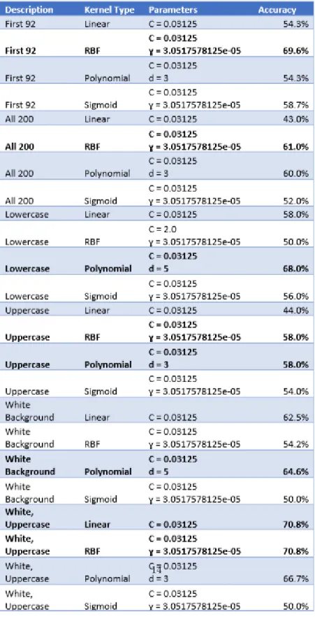
When actually running LIBSVM, I used a total of six different data sets. The first and second data sets had 92 and 200 images respectively. This included lowercase and uppercase A’s and B’s that had a white or black background and were both cursive and print. The third and fourth data sets had 50 images each of lowercase and uppercase A’s and B’s with white and black background. The fifth data sets had 50 images of A’s with white backgrounds and 50 images of B’s with white backgrounds. The final data set had 25 images each of uppercase A’s and B’s with white backgrounds. Each of these data sets was run with the four different kernels supported by LIBSVM. The parameters for each kernel were determined by a cross validation tool supported by LIBSVM.
References
[1] Ben-Hur, A & Weston, J 2010, “A User’s Guide to Support Vector Ma-chines” , Methods in Molecular Biology (Clifton, N.J.), 609, pp. 223-239, MEDLINE with Full Test, EBSCOhost
[2] Schlkopf, Bernhard, and Alexander J. Smola. Learning With Kernels : Support Vector Machines, Regularization, Optimization, And Beyond. n.p.: Cambridge, Mass. : MIT Press, c2002., 2002.
[3] Cristianini, Nello, and John Shawe-Taylor. An Introduction To Support Vector Machines : And Other Kernel-Based Learning Methods.n.p.: Cam-bridge ; New York : CamCam-bridge University Press, 2000., 2000.
[4] Chang, CC, and CJ Lin. “LIBSVM: A Library For Support Vector Ma-chines.” Acm Transactions On Intelligent Systems And Technology 2.3 (2011): Science Citation Index.
[5] Hsu, Chih-Wei, Chang, CC and CJ Lin. “A Practical Guide to Support Vector Machines” National Taiwan University 2010.