Modeling and Diagnosis of the Inter-Turn Short Circuit Fault for the Sensorless Input-Output Linearization Control of the PMSM

(1)

Cite this article as: Maanani, Y., Menacer, A. "Modeling and Diagnosis of the Inter-Turn Short Circuit Fault for the Sensorless Input-Output Linearization Control of thePMSM", Periodica Polytechnica Electrical Engineering and Computer Science, 63(3), pp. 159–168, 2019. https://doi.org/10.3311/PPee.13658

Modeling and Diagnosis of the Inter-Turn Short Circuit

Fault for the Sensorless Input-Output Linearization

Control of the

PMSM

Yacine Maanani1*_{, Arezki Menacer}1

1_{LGEB Laboratory, Department of Electrical Engineering, Faculty of Science and Technology, University of Biskra,}

Biskra University, BP 145, Biskra 07000, Algeria

*_{Corresponding author, e-mail:}_{[email protected]}

Received: 29 December 2018, Accepted: 11 February 2019, Published online: 27 March 2019 Abstract

The purpose of this paper is the inter-turn short circuit fault Modeling and detection for the sensorless input-output linearization control of the permanent magnet synchronous motor (PMSM) based on the Extended Kalman Filter observer (EKF). The fault detection procedures are based through the estimation of the stator resistance variation by the Extended Kalman Filter observer and the Fast Fourier Transformer (FFT) for the stationary state, and the Discrete Wavelet Transform (DWT) analysis of the electrical characteristics of the PMSM, for the non-stationary state. However, the FFT spectral analysis and the DWT is a useful solution to ensure that the

variation of the stator resistance estimation is caused by the inter-turn short circuit fault. The effectiveness of the sensorless control

and the fault detection techniques are presented in a simulation in MATLAB/Simulink environment.

Keywords

permanent magnet synchronous machine (PMSM), inter-turn short circuit, sensorless input-output control, fault detection, extended

kalman filter (EKF), stator resistance estimation, FFT, DWT

1 Introduction

The Permanent Magnet Synchronous Machines (PMSMs) are awarding a high attention in robotics, automotive and

electric traction due to their high efficiency, high power den

-sity and their relevance for high-performance applications by the progress in the permanent magnet materials [1, 2].

For the electric motors, the faults or failures usually lead

to serious consequences, such as intemperate downtimes, prohibitive maintenance costs, and even human casualties. The early fault detection helps in reducing the machine's maintenance cost and time. Therefore, research effort on the PMSM fault diagnosis has been on the rise [3].

The possible fault modes in the PMSM include the elec

-trical and mechanical sources. Statistics demonstrate that

over than 47 % of the electric motor failures are due to

elec-trical faults. Among them, the stator winding faults, which represent the largest portion and the most important causes of faults in the PMSM [4]; hence, an effective fault diagno

-sis is necessary to ameliorate the reliability of such motors. The early methods used noise, temperature, and vibration analysis [5, 6]. However, these methods are quite expen

-sive and its mechanical installation is sensitive to the noise.

The motor current signature analysis (MCSA) method has some advantages, like its simplicity of current measurement and its base on simple signal processing techniques, such as

the Fast Fourier transform (FFT) or similar harmonic

cal-culation procedures [7, 8]. The FFT analysis method is used

to characterize the different kinds of the short-circuit faults,

and it can be applied when the frequency is constant, unlike other algorithms which can be used in a variable speed or in

a transient state, like the Wigner Ville Distribution (WVD)

and the Wavelet Transform (WT) [9, 10].

The Wavelet theory provides a unified framework for a number of techniques which have been developed for various signal processing applications. The DWT is based on the decomposition of the signal on a basis of particu

-lar functions [11, 12]. In a variable speed control drives, the diagnosis is delicate, because the fault may appear as a disturbance for the control-loop, where the used Input-Output Linearization control corrects and compensates the fault effect, and unlike the field oriented control, the non

-linear control permits decoupling and -linearizing the sys

(2)

In the closed-loop case, the diagnosis by the approach model parametric is, therefore, necessary using observers. Multiple structures of observers have been suggested in the literature: MRAS, sliding mode observer, Luenberger observer and Extended Kalman Filter (EKF) [14, 15]. The EKF is a stochastic observer awarding the best opti

-mal estimation of states or parameters for the nonlinear systems. Many researchers have focused their attention on the uses of the EKF observer for the fault detection [16, 17].

The main objective of this paper is the detection of the inter-turn short circuit fault for the permanent magnet syn

-chronous machine driven by the sensorless input-output linearization control using the EKF observer. Three pro

-cedures of diagnosis are considered, the EKF for the sta

-tor resistance estimation while the parameters' variation is considered, the FFT method is applied for the electrical characteristic (quadratic and stator phase current) of the

PMSM in order to check if the variation is caused by the

fault or by a perturbation. Finally, the DWT analysis was introduced to overcome the shortcomings of the FFT spec

-tral analysis. The performance and the effectiveness of the proposed control and diagnosis approaches model have

been investigated through the simulation results using

MATLAB/Simulink software.

2 Dynamic model of the PMSM with an inter-turn short circuit

The stator winding faults indicate an insulation failure

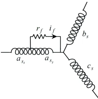
between two windings in the same phase or into different phases of the stator. Fig. 1 shows the inter-turn short circuit

fault in the stator winding of the PMSM, where the fault has

occurred in the phase (a_s) and (r_f) represents the fault resis

-tance. The sub-windings (a_s1) represent the healthy part and

(a_s₂) represent the faulty part of the phase winding [18].

The evolution of the fault resistance between r_f = ∞ and

r_f= 0 is very fast in most insulation materials. It's import

-ant to predict the inter-turn short circuit fault when it is not

highly increasing and the fault resistance is still not very

near to zero. Therefore, in the approach model, the fault

resistance is included and the machine behavior with

var-ious fault resistances is studied.

2.1 Model of the PMSM with an inter-turn short circuit fault in a, b, c coordinates

The voltage equations for the circuit of Fig. 1can be writ-ten as:

V R I L d

dt I E

s =

[ ] [ ]

s . s +

[ ] [ ]

ss s +

[ ]

s . (1)

Where: [V_s], [I_s] and [E_s] are the stator voltage, current,

and back-EMF vectors:

V_s _{= }v v v_{as bs} _cs_T I_s _{= }I I I_as _bs _cs_T E_s _{= }e e e_{as bs cs}_T .

R_s is the phase resistance and [L_ss] is the inductance matrix of the healthy state for the PMSM respectively:

R R R R L L M M M L M M M L s ss s s s s s s

[ ]

=          

[ ]

=           0 0 0 0 0 0 .

Where L_s is the self-inductance phase and M is the

mutual inductance between the phase windings for the healthy state of the PMSM. R_a₂ and L_a₂ represent respec -tively the resistance and the inductance of the faulty sub coil (a_s₂). The parameters M_a1a₂, M_a₂_b, and M_a₂ represent respectively the mutual inductances between the

sub-coil (a_s₂) and the coils (a_s₁), (b_s) and (c_s). The fault cur -rent through the fault resistance r_f is also called i_f. For the machine having one slot per pole and per phase, M_a₂_b can be considered equal to M_a₂_c.

The voltage equation of the faulty loop (a_s₂) is:

0 2 2 2 2 2 1 2 2 = − −

(

+

)

− − − + + R I L M dI dt M dI dt M dI dt e R a as a as a b bs a c cs a a a a rr I L dI dt f f a f

(

)

+ 2 . (2) Fig. 1 Equivalent model of the PMSM with an inter-turn short fault

(3)

The equations of the voltages of the three phases are thus put in the form:

V R R I L L M d dtI M M d dtI as a a b a a as a a a as a b bs =

(

+

)

+

(

+ +

)

+

(

+

)

+ 1 1 1 1 2 1 2 2 2 M M M d dtI e e R I L M d dtI V R I a c cs a f a a a f s a c a a cs 1 2 2 1 2 2 1 2 +

(

)

+

(

+

)

− −

(

+

)

= _ccs _cs _{a c} _as bs a c f s a c cs bs L d dtI M M d dtI e M d dtI M d dtI V R I + +

(

+

)

+ + − = 1 2 2 bbs bs a b as cs a b f a b cs L d dtI M M d dtI e M d dtI M d dtI + +

(

+

)

+ + −        1 2 2              . (3)

The following relations are normally allowed:

R R R R L L L M M M M M M M e e s a a a a a a a a b a b a c a c a a = = + = + + = + = + = + 1 2 1 2 1 2 1 2 1 2 1 2 ee_a2=e_a1+e_f          . (4)

By replacing the above relations Eq. (4) in the electrical equations Eq. (3), the following matrix can be written:

V V V R I I I L L L as bs cs as bs cs s s s s           =           +     0 0 0 0 0 0                 +           − + d dt I I I R I L M M as bs cs a a a a f 2 2 1 2 0 0 aa b a c f M dI dt 2 2           . (5)

2.2 Model of the PMSM with an inter-turn short circuit fault in α, β coordinates

For the star connection of the windings, the zero sequence

component of the stator current is zero. Thus, the transfor

-mation in the stator reference frame is applied:

x x x x x a b c α β       = − − −                       2 3 1 1 2 1 2 0 3 2 3 2 . (6)

In α, β coordinates, the PMSM machine equations with

an inter-turn winding fault are simplified as:

V R I L d dt I e L d dt I s f αβ αβ αβ αβ αβ   =   +     +   − ′

[ ]

0 _{ }−− ′

[ ]

R I0 f . (7)

For the faulty loop (a_s₂), the voltage equation in α, β

coordinates becomes: 0 2 3 2 3 2 1 2 2 2 1 2 2 2 2 2 = − −  + − +   _ − − R I L M M M dI dt M M a as a a a a b a c as a b a c

((

)

− − +

(

+

)

+ dI dt M dI dt e R r I L dI dt bs a c cs a f a f a f 2 2 2 2 . (8) The final equations with an inter-turn fault in α, β refer-ence frame are written as follows:

V V R V V L ddt I I e e R s s a α β α β α β α β       =       +       +      − 2₃₀ 2      − + − +       −

(

)

        I L M M M M M f a a a a b a c a b a c 2 3 2 1 2 2 1 2 2 2 2 2     dI dt f _. (9) or again: V V R R R R R I I I s a s a f f α β α β 0 0 0 0 0 2 2           = − ′ − ′ ′                     +                     + L M L M L d dt I I I e e s s a fa fa f 0 0 0 0 2 α β α β −−           ef . (10) with: ′ = = + = = −  + − +    R R R R r e e M L M M M a a f a f f fa a a a a b a c 2 2 2 2 2 1 2 2 2 2 3 2 3 2 , , _α   =

(

−

)

, . M_fβ M_{a b} M_{a c} 1 2 2 2

(4)

Since the sequence component of the current is zero,

the electromagnetic torque can be written as:

Te=e I e I e If

+ −

α α β β α2

Ω . (11)

2.3 State space form of the fault model of the PMSM

The model of the machine with the inter-turn short circuit fault Eq. (10) can be written in the state space form:

d dt I I I L M L M M L R R f fa f fa s s a s a α β β           =           − ′ − 0 0 0 0 2 1 2 2 2 0 0 0 − ′ − ′                               + − R R R I I I v e s a f f α β α α vv e ef β − β           . (12)

The state vector (x) and the input vector (u) are sup

-posed as: x I I I u v e v e e f f =           = − −           α β α α β β ; . (13)

Thus, the machine fault model Eq. (12) in the state

space form can be written as:

 x Ax Bu= + (14) with: A L M L M M L R R R R R s s a s a s a f fa f fa = −           − ′ − ′ ′    − 0 0 0 0 0 0 0 2 2 2 1 β        =           − , . B L M L M M L s s a fa f fa 0 0 0 2 1 β

3 Input-Output linearization of the PMSM

The linearization condition for checking whether the

non-linear system admits the input-output non-linearization is a rel

-ative degree of the system [19].

The degree relative to the output y x1( ) is:

 

y x

( )

=h x1

( )

=L h x_fd 1

( )

+L h x U_g 1

( )

= +f g V1 _d. (15)

X is the state vector and f, g, h are the analyticfunctions.

The relative degree r₁ = 1 gives:

  y2( )x =h2( )x =L hf 2( )x +L hg 2( )xU f= 3 (16) where : L h x g 2( )=0. Then  y x2

( )

=L h xf 2

( )

= f3.

The second derivative of the output does not involve the input U; it must derive a second time the output:

The derivative of h₂(x) dregs on g are zero, the Eq. (13)

can be written as:

y x2 h x2 L hf x L L hf g x U 2 2 2 2

( )

=

( )

=

( )

+

( )

. with: L h f L L j f L L j j f j L L x p x p x p f f d q d q f g f 2 2 1 2 2 1 3

( )

=

(

−

)

+ 

(

−

)

+        − ϕ hh L p L L j L p L L j p j x x x d d q d d q f 2 2 1 1 1

( )

= −

(

)

₊

(

−

)

+               ϕ               .

The relative degree for y₂ is r₂ = 2 and for the system is

r = r₁ + r₂ = 3.

The system is exactly linearizable (r = n = 3) where n is the order of the system.

Then the input-output relationship model is given by:

  y x y x d dtI d dt A x D x Vd Vq d 1 2 2 2

( )

      =             =

( )

+

( )

 Ω     (17) or: A L L L L x f f p j x f p j x p j f f j d q d q f

( )

= −

(

)

₊

(

−

)

+    _ −      1 1 2 2 1 3 ϕ           

( )

=

(

−

)

(

−

)

+       D g g p L L j g p L L j p j x x x f d q d q 1 1 2 2 1 0 ϕ     .

(5)

If the determinant of the decoupling matrix is not equal to zero, the control condition (NL) is defined by a relation

-ship that connects the new internal inputs (V₁, V₂) to the

physical inputs (V_d, V_q). V V D A V V x x d q       =

( )

−

( )

+            −1 1 2 . (18)

D: is the decoupling matrix.

By replacing the term for the Eq. (14) in Eq. (18), a lin

-earized and decoupled system is obtained:   y x y x d dtI d dt V V d 1 2 2 2 1 2

( )

       =             =      Ω .

4 Non-linear control for the PMSM

For checking whether a nonlinear system admits, an

input-output linearization is one degree of the system [20]:

V K I I d dtI dref d dref 1= 11

(

−

)

+ (19) or again: V K K d dt d dt d dt

dref d dref dref

1 22 21 2 2 =

(

)

+    _ − − Ω Ω Ω Ω . Ω . (20) In closed-loop, the tracking error is:

d dte K d dt e K ddte K e 1 11 2 2 2 21 2 22 2 0 0 + = + + =       (21) with: e I I e dref d ref d 1 2 = − = −     Ω Ω .

The coefficients K₁₁, K₂₁, K₂₂ are chosen so that:

P k P k P k + = + + =     11 2 21 22 0 0 . (22)

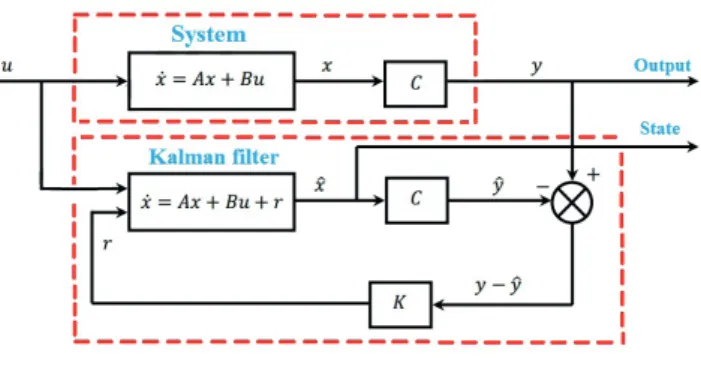
5 Extended Kalman filter observer (EKF)

The Extended Kalman Filter is a mathematical tool capa -ble of determining the quantities of the non-measura-ble

scalable states, or stating the system's parameters from the physical measurable magnitudes. In addition, the state's

measurements must show an uncorrelated noise, such as the

permanent magnet synchronous motor model [21].Fig. 2 shows the structure of the Kalman Filter observer [22].

The nonlinear stochastic systems are described by:

 x f x u w t y Cx v t =

( )

+

( )

= +

( )

    , . (System) (Measurement) (23)

Where: x is the states and u is the input of the system,

w(t) clarifies the disturbances applied to the system's input and output affected by the random noise v(t). It will be pre

-supposed that w(t) and v(t) are not linked and zero-mean

sto-chastic processes. Statistically, the stosto-chastic operation w(t) and v(t) are characterized by the covariance matrices Q and

R respectively. Therefore, Q and R can be expressed as [13]:

Q w E ww R v E vv T T =

( )

=

{ }

=

( )

=

{ }

    cov cov . ₍₂₄₎

6 Simulation of the sensorless input-output linearization control for the PMSM

The Input-Output linearizationcontrol strategy of thePMSM

is used in the simulation in the healthy and faulty states. The characteristics of the motor are given in the Appendix.

Fig. 3 presents the global diagram of the sensorless Input-Output linearization control of the PMSM using

Fig. 3 Global diagram of the sensorless Input-Output linearization

control of the PMSM

(6)

the EKF observer, based on the dynamic model of the

machine in the healthy and faulty states.

6.1 Simulation results and discussion

In order to test the effectiveness and the performance of the sensorless input-output linearization control of the PMSM in the simulation using the EKF observer, diverse tests

have been realized in the healthy and faulty states, such as

the start-up with no load and the load torque application at t = 0.5 s, then at t = 1 s in which the machine operates in

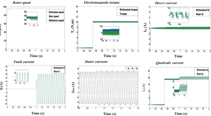
the faulty state with 3 % of the winding turns fault in the phase (a_s) where the fault resistance is r_f = 0 Ω.Fig. 4 shows the characteristics of the sensorless Input-Output lineariza

-tion control of the PMSM in the healthy and faulty states. The speed follows its reference after a transient state which lasts 0.08 s and decreases slightly at the time t = 0.5 s of the load application. A good estimated speed is noticed, where the real and estimated speeds show a perfect superposi

-tion. The electromagnetic torque presents a fast and accu

-rate dynamic, while the three phase currents illust-rate a pure sinusoidal waveform during the load application. The

estimated currents (I_d, I_q) show an accurate estimation also, the I_q current follows the evolution of the electromagnetic torque while I_d is maintained constant. At the time (t = 1 s),

3 % of the winding turns fault in the phase (a_s) where the fault resistance is r_f = 0 Ω. It's noticed that the inter-turn

short circuit fault does not affect the rotor speed and the torque responses, due to the closed-loop control which masks compensates the fault effect. The amplitude of the

fault current if after the fault occurrence is not constant and the quadratic current I_q is affected by the defect through the

appearance of the oscillations.

6.2 Stator resistance estimation via the EKF

The next test is considered for the healthy and faulty states of the PMSM operating at full load. The variation of this parameter can be exploited for the fault detection. Fig. 5

shows the estimation of R_s. The real value of the stator resis -tance decreases according to the fault considered at t = 1 s.

The results show an accurate estimation in the steady

state. Therefore, the decreasing values of the stator resistance are produced by the inter-turn short circuit; therefore, the off-line diagnosis is necessary. The next section shows the FFT analysis of the electrical characteristics of the PMSM.

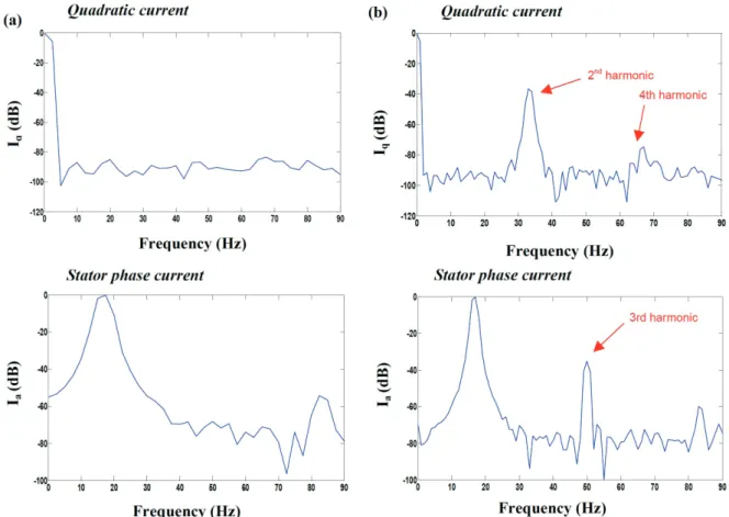
6.3 FFT analysis for the inter-turn fault diagnosis

The Fast Fourier Transformer (FFT) is known as a traditional

method for the rotary machine fault detection. The spectrum analysis is applied to the quadratic and the stator current in the healthy and faulty states of the PMSM Fig. 6. In a station -ary state, the FFT analysis is used to characterize the fault

for different numbers of the inter-turn short circuit.

Fig. 4 The electrical and a mechanical characteristics of the sensorless input-output linearization control of the PMSM in the healthy and faulty states

(7)

The measurements of the harmonic amplitudes of the stator phase current in the healthy and faulty states for the

different values of the fault severity μ = (1 %, 2 %, 3 %),

and the fault resistance r_f = (0 Ω, 5 Ω, 10 Ω) are illustrated in Table 1.

Table 1 shows the amplitudes of the harmonic increases with the severity of the fault and the inversely propor -tional to the values of the fault resistance, it can be said

that the currents became an appropriate quantity for the fault diagnosis.

The spectrum analysis with the FFT for the quadratic

current I_q shows the magnitude of the harmonic at 2 f_s which

correspond to the harmonics of defects, and the 3rd_harmonic

for the stator current increases in the faulty state. The ampli -tude of the harmonic increases with the severity of the fault

and decreases with the values of the fault resistance. Fig. 5 The evolution of the stator resistance estimation and its errors for the PMSM (a) healthy state (b) μ = 3 %, r_f= 0 Ω at t = 1 s.

(8)

6.4 DWT for the Inter-Turn short circuit fault diagnosis

The DWT is an efficient and powerful technique which pro

-vides the time-frequency representation of a non-station -ary signal with a better time resolution than the FFT [23].

Before the application of the DWT, first, we have to select the type of the mother wavelet and the number of the decomposition levels.

6.4.1 Selection of the mother wavelet

There are several wavelet families with different

mathe-matical properties that have been developed.In our case,

we have used Daubechies-44 as the mother wavelet for

the DWT analyses.

6.4.2 Specification of the Number of Decomposition levels

The decomposition level N_f depends on the sampling rate f_s

and on the frequency f. It can be calculated by the expression

N f f f int s log log .      

( )

          + 2 1 (25)

Considering f = 10000 samples/sec and f_s = 50 Hz,

the frequency bands associated with each wavelet signal are shown in Table 2.

The Daubechies wavelets of different orders are used to

decompose the stator current.

Fig. 7 shows the details and the approximation signals (d7, d8, d9, and a12) obtained by db44 in the healthy and faulty states of the machine.

Fig. 7 shows the DWT of the phase stator current, where,

the evolution of the fault is observed in the frequency

bands for the relative signal through the coefficients (a12, d7, d8, and d9). It is shown at the comparison of the details and the approximation signals when the fault resistance is fixed to 0.1 Ω and for the different values of the fault

severity μ = (1 %, 2 %, 3 %) that the amplitude of the coefficients a12 and d9 are increased due to the frequency components located at 3 f_s Table 2. Therefore, the DWT

technique is a very effective tool for the detection of the

inter-turn short circuit in the PMSM.

7 Conclusion

The studied defect in this work is the inter-turn short

cir-cuit fault in the stator winding of the permanent magnet synchronous motor (PMSM). Considering the inter-turn short circuit, a dynamic model has been presented for the control of the machine. The EKF observer is used to esti

-mate the rotor speed in both the healthy and faulty states of the machine. The estimation of the stator resistance has

been done also for the fault detection in the transient and

steady states of the PMSM.

Two signal approaches for the fault diagnosis have been

used, which are the FFT for the stationary state and the

DWT for the non-stationary state. The analyzed quantities using those two approaches are the stator current and the quadratic current. The EKF observer has an accurate esti -mation for the stator resistance R_s in both the healthy and

faulty states.Furthermore, it can be employed as a fault indicator in the transient and steady states.

The FFT and the DWT analyses have been used to

con-firm if the variation of the stator resistance is occurred due to the inter-turn fault or by the load application or any other external disturbances. It should be noted that the stator phase

current and the quadratic current gave good informations

about the presence of the fault, unlike the rotor speed, which has been affected by the closed-loop control regulation.

The FFT analysis has advantages in the steady state

only. Hence, the use of the DWT method is a very effec -tive and reliable technique for the diagnosis and detection of the inter-turn short circuit fault in the PMSM, in which

the failure can be detected while the motor is operating, particularly in the case of the inter-turn fault.

Table 1 The FFT analysis of the stator and quadratic currents for the different values of the severity of the fault and fault resistance Severity of fault with rf = 0.1 Ω Faulty resistances with μ = 3 %

1 % 2 % 3 % 10 Ω 5 Ω 0 Ω 3rd_{harmonic of "}_I sa" in Healthy sate −73.53 −73.53 −73.53 −73.53 −73.53 −73.53 3rd_{harmonic of "}_I sa"in Faulty state −47.42 −34.67 −30.87 −60.53 −55.46 −30.93 2nd_{harmonic of "}_I q" in Healthy state −89.87 −89.87 −89.87 −89.87 −89.87 −89.87 2nd_{harmonic of "}_I q" in Faulty state −49.92 −41.37 −35.29 −73.49 −54.64 −36.55

Table 2The frequency levels of the wavelet coefficients.

Level Frequency band (Hz)

a12 0 – 1.22

d9 09.765 – 19.531

d8 19.531 – 39.062

(9)

Appendix

PMSM parameters used in the simulation results:

P_n Rated power 5 kW

I_n Rated current 19 A

p Number of pole pairs 4

N_s Winding turn no. / slot 40

R_s Stator resistance 0.88 Ω

L_s Stator inductance 2.82 mH

Ω_s Synchronous speed 1000 rpm

J Inertia moment 0.0006 kg.m2 f Coefficient of damping 0.007 Nm/rad/s Φ_f Flux established by rotor 0.108 Wb Fig. 7 The DWT analysis of the stator current envelope: (a) Healthy state, (b) Faulty state μ = 1 %, rf = 0.1 Ω (c) Faulty stateμ = 2 %, rf= 0.1 Ω

(d) Faulty state μ = 3 %, rf = 0.1 Ω

References

[1] Bechkaoui, A., Ameur, A., Bouras, S., Ouamrane, K. "Hybrid Control Using Adaptive Fuzzy Sliding Mode for Diagnosis of Stator Fault in PMSM", Periodica Polytechnica Transportation Engineering, 44(3), pp. 172–180, 2016.

https://doi.org/10.3311/PPtr.8242

[2] Huangfu, Y., Wang, S., Wang, S., Li, H., Yuan, D., Wang, S., Di Rienzo, L. "Macro-modeling and passivity enforcement for PMSM winding", COMPEL - The international journal for com

-putation and mathematics in electrical and electronic engineering, 36(6), pp. 1729–1738, 2017.

https://doi.org/10.1108/COMPEL-12-2016-0572

[3] Kiselev, A., Kuznietsov, A., Leidhold, R. "Model based online

detection of inter-turn short circuit faults in PMSM drives under

non-stationary conditions", In: 2017 11th_{IEEE International} Conference on Compatibility, Power Electronics and Power Engineering, CPE-POWERENG, Cadiz, Spain, 2017, pp. 370–374.

https://doi.org/10.1109/CPE.2017.7915199

[4] Vajsz, T., Számel, L., Rácz, G. "A Novel Modified DTC-SVM Method with Better Overload-capability for Permanent Magnet

Synchronous Motor Servo Drives", Periodica Polytechnica Electrical

Engineering and Computer Science, 61(3), pp. 253–263, 2017.

(10)

[5] Keskes, H., Braham, A. "Recursive Undecimated Wavelet Packet Transform and DAG SVM for Induction Motor Diagnosis", IEEE Transactions on Industrial Informatics, 11(5), pp. 1059–1066, 2015.

https://doi.org/10.1109/TII.2015.2462315

[6] Kalas, D., Pretl, S., Reboun, J., Soukup, R., Hamacek, A.

"Novel Technology for Thermal Testing of Glove", Periodica

Polytechnica Electrical Engineering and Computer Science, 62(4), pp. 165–171, 2018.

https://doi.org/10.3311/PPee.13264

[7] Farkas, B., Veszprémi, K. "Regenerative Cascaded Cell Inverter with Active Filter", Periodica Polytechnica Electrical Engineering and Computer Science, 59(2), pp. 36–42, 2015.

[8] Pálfi, V., Kollár, I. "Limitations of the noise model of round off for the FFT", Periodica Polytechnica Electrical Engineering, 53(3-4), pp. 179–185, 2010.

https://doi.org/10.3311/pp.ee.2009-3-4.09

[9] Wang, Y., Zhang, F., Zhang, S., Yang, G. "A novel diagnostic algorithm for AC series arcing based on correlation analysis of high-frequency component of wavelet", COMPEL - The interna

-tional journal for computation and mathematics in electrical and electronic engineering, 36(1), pp. 271–288, 2017.

[10] Égető, T., Farkas, B. "Model Reference Adaptive System for the Online Rotor Resistance Estimation in the Slip-Ring Machine

Based Test-bench", Periodica Polytechnica Electrical Engineering

and Computer Science, 62(4), pp. 149–154, 2018.

[11] Bessous, N., Zouzou, S. E., Bentrah, W., Sbaa, S., Sahraoui, M.

"Diagnosis of bearing defects in induction motors using discrete

wavelet transform", International Journal of System Assurance Engineering and Management, 9(2), pp. 335–343, 2018.

https://doi.org/10.1007/s13198-016-0459-6

[12] de Alencar, R. J. N., Ferreira, A. M. D. "Transformer Inrush Currents and Internal Faults Identification in Power Transformers Using Wavelet Energy Gradient", Journal of Control, Automation and Electrical Systems, 27(3), pp. 339–348, 2016.

https://doi.org/10.1007/s40313-016-0236-4

[13] Ahmed, M., Karim, F. M. "Input-output linearization and sliding mode control of a permanent magnet synchronous machine fed by a three levels inverter", Journal of electrical engineering, 57(4), pp. 205–210, 2006.

[14] Virosztek, T., Kollár, I. "Theoretical Limits of Parameter Estimation

Based on Quantized Data", Periodica Polytechnica Electrical

Engineering and Computer Science, 61(4), pp. 312–319, 2017.

[15] Ameid, T., Menacer, A., Talhaoui, H., Harzelli, I., Ammar, A. "Simulation and real-time implementation of sensorless field

oriented control of induction motor at healthy state using rotor

cage model and EKF", In: Proceedings of 2016 8th_{International} Conference on Modelling, Identification and Control, ICMIC 2016, Algiers, Algeria, 2017, pp. 695–700.

https://doi.org/10.1109/ICMIC.2016.7804201

[16] Talla, J., Peroutka, J., Blahnik, V., Streit, L. "Rotor and Stator Resistance Estimation of Induction Motor Based on Augmented EKF", In: 2015 International Conference on Applied Electronics (AE), Pilsen, Czech Republic, 2015, pp. 253–258.

[17] Kojabadi, H. M., Abarzadeh, M., Chang, L. "A Comparative Study of Various Methods of IM's Rotor Resistance Estimation", In: 2015 IEEE Energy Conversion Congress and Exposition (ECCE), Montreal, QC, Canada, 2015, pp. 2884–2891.

https://doi.org/10.1109/ECCE.2015.7310064

[18] Vaseghi, B., Takorabet, N. "Modelling and study of PM machines with inter-turn fault dynamic model – FEM model", Electric Power Systems Research, 81(8), pp. 1715–1722, 2011.

https://doi.org/10.1016/j.epsr.2011.03.017

[19] Harnefors, L., Hinkkanen, M. "Stabilization Methods for Sensorless Induction Motor Drives-A Survey", IEEE Journal of Emerging and Selected Topics in Power Electronics, 2(2), pp. 132–142, 2014.

https://doi.org/10.1109/JESTPE.2013.2294377

[20] Titaouine, A., Moussi, A., Benchabane, F., Yahia, K. "Sensorless

Nonlinear Control of Permanent Magnet Synchronous Motor

Using the Extended Kalman Filtre", Asian Journal of Information Ttechnology, 5(12), pp. 1416–1422, 2006. [online] Available at:

http://medwelljournals.com/abstract/?doi=ajit.2006.1416.1422

[Accessed: 05 December 2006]

[21] Janiszewski, D., Muszyński, R. "Sensorless control of PMSM drive with state and load torque estimation", COMPEL - The International Journal for Computation and Mathematics in Electrical and Electronic Engineering, 26(4), pp. 1175–1187, 2007.

https://doi.org/10.1108/03321640710756483

[22] Ameid, T., Menacer, A., Talhaoui, H., Harzelli, I. "Rotor resistance estimation using Extended Kalman filter and spectral analysis for

rotor bar fault diagnosis of sensorless vector control induction

motor", Measurement: Journal of the International Measurement Confederation, 111, pp. 243–259, 2017.

https://doi.org/10.1016/j.measurement.2017.07.039

[23] Sakhara, S., Saad, S., Nacib, L. "Diagnosis and detection of short circuit in asynchronous motor using three-phase model", International Journal of System Assurance Engineering and Management, 8(2), pp. 308–317, 2016.

. https://doi.org/10.3311/PPee.13658