An analysis of deep neural networks for texture classification

(1)

LUIZ GUSTAVO HAFEMANN

AN ANALYSIS OF DEEP NEURAL NETWORKS FOR

TEXTURE CLASSIFICATION

Dissertation presented as partial requisite to obtain the Master’s degree. M.Sc. pro-gram in Informatics, Universidade Federal do Paran´a.

Advisor: Prof. Dr. Luiz Eduardo S. de Oliveira

Co-Advisor: Dr. Paulo Rodrigo Cavalin

CURITIBA 2014

(2)

AN ANALYSIS OF DEEP NEURAL NETWORKS FOR

TEXTURE CLASSIFICATION

Dissertation presented as partial requisite to obtain the Master’s degree. M.Sc. pro-gram in Informatics, Universidade Federal do Paran´a.

Advisor: Prof. Dr. Luiz Eduardo S. de Oliveira

Co-Advisor: Dr. Paulo Rodrigo Cavalin

CURITIBA 2014

(3)

ACKNOWLEDGMENTS

I would like to thank my wife, Renata, for all the love, patience and understanding during the last two years. I also want to thank my parents, for all the support during this time, and during all my life. I would like to thank my research advisor, Dr. Luiz Oliveira, and my co-advisor Dr. Paulo Cavalin, for all the guidance and assistance during this time. Last but not least, I would like to thank Dennis Furlaneto for all the reviews of my dissertation, and for the regular discussions in the coffee area, from where many ideas emerged.

(4)

LIST OF FIGURES

2.1 A single artificial neuron. . . 7

2.2 A neural network composed of three layers. . . 8

2.3 Architecture of a convolution network for traffic sign recognition [36]. . . . 14

2.4 Sample feature maps learned by a convolution network for traffic sign recog-nition [36] . . . 15

2.5 The forward propagation phase of a convolutional layer. . . 16

2.6 The forward propagation phase of a pooling layer. . . 17

2.7 Transfer learning from the ImagetNet dataset to the Pascal VOC dataset . 21 4.1 An overview of the Pattern Recognition process. . . 27

4.2 The zoning methodology used by Costa [56]. . . 30

4.3 The Deep Convolutional Neural Network architecture. . . 33

4.4 The training procedure using random patches . . . 36

4.5 The testing procedure using non-overlapping patches . . . 38

4.6 The training procedure for transfer learning . . . 40

4.7 The testing procedure for transfer learning . . . 41

5.1 Error rates on the Forest Species dataset with Macroscopic images, for CNNs trained with different hyperparameters. . . 43

5.2 Error rates on the Forest Species dataset with Microscopic images, for CNNs trained with different hyperparameters. . . 44

5.3 Random predictions for patches on the Testing set (Macroscopic images) . 45 5.4 Random predictions for patches on the Testing set (Microscopic images) . . 46

5.5 Filters learned by the first convolutional layers of models trained on the Macroscopic images dataset. . . 47

5.6 Filters learned by the first convolutional layer of a model trained on the Microscopic images dataset. . . 47

(8)

5.7 Error rates on the IAM dataset, for CNNs trained with different hyperpa-rameters. . . 50 5.8 Error rates on the BFL dataset, for CNNs trained with different

hyperpa-rameters. . . 51 5.9 Random predictions for patches on the IAM Testing set . . . 52 5.10 Random predictions for patches on the BFL Testing set . . . 52 5.11 Filters learned by the first convolutional layer of a model trained on the

IAM dataset. . . 53 5.12 Filters learned by the first convolutional layer of a model trained on the

BFL dataset. . . 53 5.13 Error rates on the Latin Music Dataset, for CNNs trained with different

hyperparameters. . . 55 5.14 Random predictions for test patches on the Latin Music Dataset . . . 56 5.15 Filters learned by the first convolutional layer of a model trained on the

Latin Music dataset. . . 56 5.16 Error rates on the Brodatz dataset, for CNNs trained with different

hyper-parameters. . . 59 5.17 Random predictions for patches on the Brodatz-32 Testing set . . . 60 5.18 Filters learned by the first convolutional layer of a model trained on the

Brodatz-32 dataset. . . 60 A.1 Sample images from the macroscopic Brazilian forest species dataset . . . . 66 A.2 Sample images from the microscopic Brazilian forest species dataset . . . . 67 A.3 Sample texture created from the Latin Music Dataset dataset. . . 67 A.4 Sample image from the BFL dataset, and the associated texture. [53] . . . 68 A.5 Sample image from the IAM dataset, and the associated texture. [8] . . . . 68 A.6 Sample images from the Brodatz-32 dataset [58] . . . 69

(9)

LIST OF TABLES

3.1 Comparison of top published results on the CIFAR-10 dataset . . . 26

4.1 Summary of the properties of the datasets . . . 31

5.1 Classification on the Macroscopic images dataset . . . 48

5.2 Classification on the Microscopic images dataset . . . 48

5.3 Classification on the IAM dataset . . . 53

5.4 Classification on the BFL dataset . . . 54

5.5 Classification on the Latin Music dataset . . . 57

5.6 Confusion Matrix on the Latin Music Dataset classification (%) - Our method 58 5.7 Confusion Matrix on the Latin Music Dataset classification (%) - Costa et al.[9] . . . 58

5.8 Classification on the Brodatz-32 dataset . . . 61

5.9 Classification on the Macroscopic Forest species dataset . . . 62

(10)

RESUMO

Classifica¸cão de texturas é um problema na área de Reconhecimento de Padrões com uma ampla gama de aplica¸cões. Esse problema é geralmente tratado com o uso de descritores de texturas e modelos de reconhecimento de padrões, tais como Máquinas de Vetores de Suporte (SVM) e Regra dos K vizinhos mais próximos (KNN).

O método clássico para endere¸car o problema depende do conhecimento de especialis-tas no dom´ınio para a cria¸cão de extratores de caracter´ısticas relevantes (discriminantes), criando-se vários descritores de textura, cada um voltado para diferentes cenários (por exemplo, descritores de textura que são invariantes à rota¸cão, ou invariantes ao borra-mento da imagem). Uma estratégia diferente para o problema é utilizar algoritmos para aprender os descritores de textura, ao invés de constru´ı-los manualmente. Esse é um dos objetivos centrais de modelos de Arquitetura Profunda – modelos compostos por múltiplas camadas, que tem recebido grande aten¸cão nos últimos anos. Um desses métodos, cha-mado de Rede Neural Convolucional, tem sido utilizado para atingir o estado da arte em vários problemas de visão computacional como, por exemplo, no problema de reconheci-mento de objetos. Entretanto, esses métodos ainda não são amplamente explorados para o problema de classifica¸cão de texturas.

A presente disserta¸cão preenche essa lacuna, propondo um método para treinar Redes Neurais Convolucionais para problemas de classifica¸cão de textura, lidando com os desafios e tomando em considera¸cão as caracter´ısticas particulares desse tipo de problema. O método proposto foi testado em seis bases de dados de texturas, cada uma apresentando um desafio diferente, e resultados próximos ao estado da arte foram observados para a maioria das bases, obtendo-se resultados superiores em duas das seis bases de dados.

Por fim, é apresentado um método para transferência de conhecimento entre diferen-tes problemas de classifica¸cão de texturas, usando Redes Neurais Convolucionais. Os experimentos conduzidos demonstraram que essa técnica pode melhorar o desempenho dos classificadores em problemas de textura com bases de dados pequenas, utilizando o

(11)

conhecimento aprendido em um problema similar, que possua uma grande base de dados.

Palavras chave: Reconhecimento de padr˜oes; Classifica¸c˜ao de Texturas; Redes Neu-rais Convolucionais

(12)

ABSTRACT

Texture classification is a Pattern Recognition problem with a wide range of applications. This task is commonly addressed using texture descriptors designed by domain experts, and standard pattern recognition models, such as Support Vector Machines (SVM) and K-Nearest Neighbors (KNN).

The classical method to address the problem relies on expert knowledge to build rel-evant (discriminative) feature extractors. Experts are required to create multiple texture descriptors targeting different scenarios (e.g. features that are invariant to image rota-tion, or invariant to blur). A different approach for this problem is to learn the feature extractors instead of using human knowledge to build them. This is a core idea behind Deep Learning, a set of models composed by multiple layers that are receiving increased attention in recent years. One of these methods, Convolutional Neural Networks, has been used to set the state-of-the-art in many computer vision tasks, such as object recognition, but are not yet widely explored for the task of texture classification.

The present work address this gap, by proposing a method to train Convolutional Neural Networks for texture classification tasks, facing the challenges of texture recogni-tion and taking advantage of particular characteristics of textures. We tested our method on six texture datasets, each one posing different challenges, and achieved results close to the state-of-the-art in the majority of the datasets, surpassing the best previous results in two of the six tasks.

We also present a method to transfer learning across different texture classification problems using Convolutional Neural Networks. Our experiments demonstrated that this technique can improve the performance on tasks with small datasets, by leveraging knowledge learned from tasks with larger datasets.

Keywords: Pattern Recognition; Texture Classification; Convolutional Neural Net-works

(13)

CHAPTER 1 INTRODUCTION

Texture classification is an important task in image processing and computer vision, with a wide range of applications, such as computer-aided medical diagnosis [1], [2], [3], clas-sification of forest species [4], [5], [6], clasclas-sification in aerial/satellite images [7], writer identification and verification [8] and music genre classification [9].

Texture classification commonly follows the standard procedure for pattern recogni-tion, as described by Bishop et al. in [10]: extract relevant features, train a model using a training dataset, and evaluate the model on a held-out test set.

Many methods have been proposed for the feature extraction phase on texture clas-sification problems, as reviewed by Zhang et al. [11] and tested on multiple datasets by Guo et al. [12]. Noteworthy techniques are: Gray-Level Co-occurrence Matrices (GLCM), the Local Binary Pattern operator (LBP), Local Phase Quantization (LPQ), and Gabor filters.

The methods above rely on domain experts to build the feature extractors to be used for classification. An alternative approach is to use models that learn directly from raw

data, for instance, directly from pixels in the case of images. The intuition is using such methods to learn multiple intermediate representations of the input, in layers, in order to better represent a given problem. Consider an example for object recognition in an image: the inputs for the model can be the raw pixels in the image. Each layer of the model constitutes an equivalent of feature detectors, transforming the data into more abstract (and hopefully useful) representations. The initial layers can learn low-level features, such as detecting edges, and subsequent layers learn higher-level representations, such as detecting more complex local shapes, up to high-level representations, such as recognizing a particular object [13]. In summary, the term Deep Learning refers to machine learning models that have multiple layers, and techniques for effectively training these models,

(14)

commonly building Deep Neural Networks or Deep Belief Networks [14], [15].

Methods using deep architectures have set the state-of-the-art in many domains in recent years, as reviewed by Bengio in [13] and [16]. Besides improving the accuracy on different pattern recognition problems, one of the fundamental goals of Deep Learning is to move machine learning towards the automatic discovery of multiple levels of represen-tation, reducing the need for feature extractors developed by domain experts [16]. This is especially important, as noted by Bengio in [13], for domains where the features are hard to formalize, such as for object recognition and speech recognition tasks.

In the task of object recognition, deep architectures have been widely used to achieve state-of-the-art results, such as in the CIFAR dataset[17] where the top published re-sults use Convolutional Neural Networks (CNN) [18]. The tasks of object and texture classification present similarities, such as the strong correlation of pixel intensities in the 2-D space, and present some differences, such as the ability to perform the classification using only a relatively small fragment of a texture. In spite of the similarities with object classification we observe that deep learning techniques are not yet widely used for tex-ture classification tasks. Kivinen and Williams [19] used Restricted Boltzmann Machines (RBMs) for texture synthesis, and Luo et al. [20] used spike-and-slab RBMs for texture synthesis and inpainting. Both consider using image pixels as input, but they do not consider training deep models for classification among several classes. Titive et al. [21] used convolutional neural networks on the Brodatz texture dataset, but considered only low resolution images, and a small number of classes.

The similarities between texture classification and object recognition, and the good results demonstrated by using deep architectures for object recognition suggest that these techniques could be successfully applied for texture classification.

1.1 Motivation

There is a considerable set of potential applications for texture recognition, as briefly presented above. However, despite the reported success of classical texture classification techniques in many of these tasks, these problems are still not resolved and are subject

(15)

of active research, with potential to increase recognition rates.

A second motivation is that traditional machine learning techniques often require human expertise and knowledge to hand-engineer features, for each particular domain, to be used in classification and regression tasks. It can be considered that the actual intelligence in such systems is therefore in the creation of such features, instead of the machine learning algorithm that uses them. Therefore, using techniques that do not rely on expert-defined feature extractors can make it easier to develop effective machine learning models for novel datasets, without requiring the test and selection of a large set of possible feature extractors.

1.2 Challenges

Here is a set of challenges in applying deep learning techniques to texture classification problems:

• Image size: The majority of the image-related tasks where deep learning was success-fully applied used images of small size. Examples: MNIST (28x28 pixels), STL-10 (96x96), Norb (108x108), Cifar-10 and Cifar-100 (32x32).

• Model size and Training time: One exception to dataset list above is the ImageNet dataset, which consists in high-resolution images of variable sizes. The best results on this dataset, however, require significant usage of computer resources (such as 16 thousands cores running for three days [22]). The texture datasets commonly consist of higher resolution images, and therefore different techniques need to be tested, in order to classify the textures without using too much computing resources.

1.3 Objectives

The main objective of this research is to test whether or not deep learning models, in particular Convolutional Neural Networks, can be successfully applied for texture classi-fication problems.

(16)

More specifically, we test these methods on multiple texture datasets, developing a method to cope with the high-resolution texture images without requiring models that are too large, or that require too much computing power to train. Six texture datasets were selected for testing, representing different domain problems, and containing different characteristics, such as image sizes, number of classes and number of samples per class. As part of this effort, we assess if it is possible to obtain a generic framework that brings good results for multiple texture problems.

After training the models on each dataset, the accuracy of the deep models are com-pared with the state-of-the-art results achieved using the classical texture descriptors.

Finally, another objective of this research is to evaluate a method of Transfer Learning for texture classification. Transfer Learning consists in using a model trained in one task to improve results on another task. This is particularly interesting when using Deep Neural Networks, as these models often require large datasets to be effectively trained. We investigate the hypothesis that we can leverage a neural network trained on a large dataset to improve the results on other tasks, including tasks with smaller datasets.

1.4 Contributions

In this dissertation, we propose a method to train Convolutional Neural Networks on texture classification datasets. We explore the hypothesis that, for most textures, we can classify a texture using only a small fragment of the image. This allowed us to use datasets with large images and still keep the neural network models with a reasonable size. It also enabled us to use a strategy of classifying parts of the images individually, and subsequently combine the results of multiple predictions of the same texture image, achieving good results. We validated our method using six texture datasets, each one posing different challenges. The proposed method obtained excellent results for some types of tasks (in particular, tasks with large datasets), achieving state-of-the-art performance. We also propose a method to transfer learning across texture classification tasks, using a Convolutional Neural Network. We explore the idea that the weights learned by a Convolutional Neural Network can be used similarly to feature extractors, evaluating the

(17)

hypothesis that the features learned by the model in one dataset can be relevant for other tasks. We explore this idea by using a CNN trained in one dataset to improve the performance on a task with another dataset. We validated this proposal in four experiments, considering both cases where the tasks are from similar domains, and cases where the tasks are from different domains. We found that the method for transfer learning was particularly useful to improve the performance on tasks with small datasets, even when transfer knowledge to a task from a different domain.

The remainder of this dissertation is organized as follows. We present the theoretical background of neural networks and transfer learning in Chapter 2. In Chapter 3 we review the state-of-the-art of using deep neural networks for a similar task: object recognition. In Chapter 4, we present our method for training CNNs for texture classification, and the method to transfer learning across texture classification tasks. The experimental evaluation is presented in Chapter 5, and we conclude our work in Chapter 6. Appendix A lists samples from the texture datasets used in the experimental evaluation.

(18)

CHAPTER 2 THEORETICAL BACKGROUND

To make this document self-contained, this Chapter reviews the theoretical foundations for Deep Neural Networks. The basic concepts of Artificial Neural Networks are presented, starting with the original models that date back from 1943. The concept of Deep Neural networks is then reviewed, with the recent advancements in the field that enabled training Deep Neural Networks successfully. Afterwards, we review the theoretical foundations of other procedures and methods used in the present work: the combination of multiple classifiers, and transferring knowledge across different learning tasks.

2.1 Artificial Neural Networks

Artificial Neural Networks are mathematical models that use a collection of simple compu-tational units, called Neurons, interlinked in a network. These models are used in a variety of pattern recognition tasks, such as speech recognition, object recognition, identification of cancerous cells, among others [23]

Artificial Neural Networks date back to 1943, with work by McCulloch and Pitts [24]. The motivation for studying neural networks was the fact that the human brain was superior to a computer at many tasks, a statement that holds true even today for tasks such as recognizing objects and faces, in spite of the huge advances in the processing speed in modern computers.

2.1.1 Artificial Neuron

The neuron is the basic unit on Artificial Neural Networks, and it is used to construct more powerful models. A typical set of equations to describe Neural Networks is provided in [25], and is listed below for completeness. A single neuron implements a mathematical function given its inputs, to provide an output, as described in equation 2.1 and illustrated

(19)

Figure 2.1.

input 1 output

bias

input 2

Figure 2.1: A single artificial neuron.

f(x) =σ(

n X

i=1

xiwi+b) (2.1)

In this equation, xi is the input i, wi is the weight associated with input i, b is a

bias term and σ is a non-linear function. Common non-linear functions are the sigmoid function (described in 2.2), and the Hyperbolic tangent function (tanh).

σ(x) = 1

1 +e−x (2.2)

More recently, a new and simple type of non-linearity has been proposed, called Recti-fied Linear Units (ReLU). Tests conducted by Krizhevsky in [26] reported convergence 6 times faster by using ReLU activations compared to equivalent networks withtanhunits. This non-linearity is described in equation 2.3

σ(x) =max(0, x) (2.3)

2.1.2 Multi-layer Neural Networks

Models based on a single neuron, also called Perceptrons, have severe limitations. As noted by Minsky and Papert [27], a perceptron cannot model data that is not linearly separable, such as modelling a simple XOR operator. On the other hand, as shown by Hornik et al. [28], Multi-layer Neural Networks are universal approximators, that is: they can approximate any measurable function to any desired degree of accuracy.

(20)

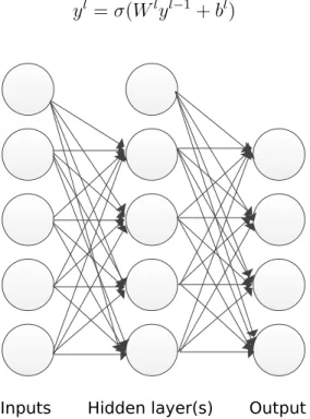
A Multi-layer Neural network consists of several layers of neurons. The first layer is composed of the inputs to the neural network, it is followed by one or morehidden layers, up to a last layer that contains the outputs of the network. In the simplest configuration, each layerl is fully connected with the adjacent layers (l−1 andl+ 1), and produces an output vectoryl _{given the output vector of the previous layer}_yl−1_{. The output of a layer}

is calculated by applying the neuron activation function for all neurons on the layer, as noted in equation 2.4, where Wl is a matrix of weights assigned to each pair of neurons from layer l and l−1, and bl _{is a vector of bias terms for each neuron in layer}_l_.

yl =σ(Wlyl−1+bl) (2.4)

Inputs Hidden layer(s) Output

Figure 2.2: A neural network composed of three layers.

2.1.2.1 Forward Propagation

The phase calledforward propagation consists in applying the neuron activation equation (2.1) starting from first hidden layer, up to the output layer. For classification tasks, the output layer commonly uses another activation function, called Softmax. Softmax is particularly useful for the last layer as the function generates a well-formed probability distribution on the outputs. The softmax equation is defined below (2.5 and 2.6). In

(21)

these equations, zl

i is the output of the layer (for neuron i) before the application of the

non-linearity, yl

i is the output of the layer for the neuron i, Wil is a vector of weights

connecting each neuron on layer l−1 to the neuron i on layer l and bl

i is a bias term for

the neuron. The summation term considers all neuronsj on the layer l.

zli =Wilyl−1+bli (2.5) yil = ezl i P je zl j (2.6)

2.1.2.2 Training Objective

In order to train the model, an error function, also called loss function, is defined. This function calculates the error of the model predictions with respect to a dataset. The objective of the training is to minimize the sum (or, equivalently, minimize the mean) of this error function applied to all examples in the dataset. Commonly used loss functions are the Squared Error function (SE), described in equation 2.7, and the Cross-Entropy error function (CE), described in equation 2.8 (both equations describe the error for a single example in the dataset). As analyzed by Golik et al [29], it can be shown that the true posterior probability is a global minimum for both functions, and therefore a Neural Network can be trained by minimizing either. On the other hand, in practice using Cross-Entropy error leads to faster convergence, and therefore this error function became more popular in recent years.

E = 1 2 X c (y_cl−tc)2 (2.7) E =−X c (tclogycl)2 (2.8)

In these equations, ycl is the output of unit c in the last layer in the model (l), and tc

(22)

tc =        1, if t=c 0, otherwise (2.9)

2.1.2.3 Backpropagation

The error function can be minimized using Gradient-Based Learning. This strategy con-sists in taking partial derivatives of the error function with respect to the model pa-rameters, and using these derivatives to iteratively update the parameters [30]. Efficient learning algorithms can be used for this purpose if these gradients (partial derivatives) can be computed analytically.

The phase called backpropagation consists in calculating the derivatives of the error function with respect to the model’s parameters (weights and biases), by propagating the error from the output layers, back to the initial layers, one layer at a time. Since each layer in the Neural Network consists of simple functions using only the values from the previous layer, we can use the chain rule to easily determine the derivatives analytically. For instance, to calculate the gradient respective to the weights in a layer we have the equation below, as described in [31]:

δE δwhj = δE δyi δyi δzh δzh δwhj (2.10) Where yi is the output of the neuron, zh is the output before applying the activation

function, and whj’s are the weights.

In order to use this strategy, we need to calculate:

1. The derivative of the error with respect to the neurons in the last layer δE δyL

i

2. The derivative of the outputs yi with respect to the outputs before the activation

functionzi, that is δyl

i

δzl i

3. The derivative of zj with respect to the weights wij, that is δzl

j

δwl i,j

4. The derivative of zj with respect to the bias bj, that is δzl

j

δbl j

(23)

5. The derivative of zj with respect to its inputs, that is δzl

j

δyl−1 i

We start with the top layer, calculating the derivative of the error (Cross-Entropy) with respect tozi. In this equation,ti is defined as above (in equation 2.9):

δE δzl i

=yl_i−ti (2.11)

For the derivatives with respect to the weights, we obtain the formula:

δzl j

δwl ij

=y_il−1 (2.12)

For the derivatives with respect to the biases, we obtain the formula:

δzl j

δbl i

= 1 (2.13)

For the derivatives with respect to the inputs, we obtain the formula:

δzl j

δy_il−1 =w

l

ij (2.14)

The equations above are sufficient to compute the derivatives with respect to the weights and biases of the last layer, and the derivative with respect to the outputs of the layer l−1. The other equation necessary is the derivative of the activation function of the layers 1 until l−1 (that don’t use softmax). The derivative for the sigmoid function is described below: δyl i δzl i =y_il(1−yl_i) (2.15)

2.1.2.4 Training algorithm

Training the network consists in minimizing the error function (by updating the weights and biases), often using the Stochastic Gradient Descent algorithm (SGD), or quasi-Newton methods, such as L-BFGS (Limited memory Broyden-Fletcher-Goldfarb-Shanno

(24)

algorithm).

The SGD algorithm, as defined in [32], is described below at a high-level. The inputs are: W - the weights and biases of the network, (X, y) - the dataset, batch size - the number of training examples that are used in each iteration, and α, the learning rate. For notation simplicity, all the model parameters are represented inW. In practice, each layer usually defines a 2-dimensional weight matrix and a 1-dimensional bias vector. In summary, SGD iterates over mini-batches of the dataset, performing forward-propagation followed by a back-propagation to calculate the error derivatives with respect to the parameters. The weights are updated using these derivatives and a new mini-batch is used. This procedure is repeated until a convergence criterion is reached. Common convergence criteria are: a maximum number ofepochs (number of times that the whole training set was used); a desired value for the cost function is reached; or training until the cost function shows no improvement in a number of iterations.

Algorithm 1Stochastic Gradient Descent

Require: W, X, y, batch size, α W ← random values

repeat

x batch, y batch ← next batch size examples in (X, y)

network state ← ForwardProp(W, x batch)

Wgrad ← BackProp(network state, y batch)

∆W ← −αWgrad

W ←W + ∆W

until Convergence Criteria()

One of the potential problems with stochastic gradient descent is having oscillations in the gradient, since not all examples are used for each calculation of the derivatives. This can cause slow convergence of the network. One strategy to mitigate this problem is the use of Momentum. The idea is to take the running average of the derivatives, by incorporating the previous update ∆W in the update for the current iteration. The equation for momentum is defined in equation 2.16 [31]. In this equation ∆wt _{refers to}

(25)

the update to the weights in iteration t, and β is a factor for the momentum, usually taken between 0.5 and 1.0 [31].

∆w(_ijt)=−αδE

(t)

δwi

+β∆w_ij(t−1) (2.16)

2.2 Training Deep Neural Networks

The depth of an architecture refers to the number of non-linear operations that are com-posed on the network. While many of the early successful applications of neural networks used shallow architectures (up to 3 levels), the mammal brain is organized in a deep ar-chitecture. The brain appears to process information through multiple stages, which is particularly clear in the primate visual system[13]. Deep Neural Networks have been in-vestigated for decades, but training deep networks consistently yielded poor results, until very recently. It was observed in many experiments that deep networks are harder to train than shallow networks, and that training deep networks often get stuck in apparent local minima (or plateaus) when starting with random initialization of the network parameters. It was discovered, however, that better results could be achieved by pre-training each layer with an unsupervised learning algorithm [14]. In 2006, Hinton obtained good results using Restricted Boltzmann Machines (a generative model) to perform unsupervised training of the layers [14]. The goal of this training was to obtain a model that could capture patterns in the data, similarly to a feature descriptor, not using the dataset labels. The weights learned by this unsupervised training were then used to initialize neural networks. Similar results were reported using auto-encoders for training each layer [15]. These ex-periments identified that layers could be pre-trained one at a time, in a greedy layer-wise format. After the layers are pre-trained, the learned weights are used to initialize the neural network, and then the standard back-propagation algorithm is used for fine-tuning the network. The advantage of unsupervised pre-training was demonstrated in several statistical comparisons [15], [33], [34], until recently, when deep neural networks trained only with supervised learning started to register similar results in some tasks (like object recognition). Ciresan et al. [18] demonstrate that properly trained deep neural networks

(26)

(with only supervised learning) are able to achieve top results in many tasks, although not denying that pre-training might help, especially in cases were little data is available for training, or when there are massive amounts of unlabeled data.

On the task of image classification, the best published results use a particular type of architecture calledConvolutional Neural Network, which is described in the next section.

2.3 Convolutional Neural Networks

Convolutional networks combine three architectural ideas: local receptive fields, shared (tied) weights and spatial or temporal sub-sampling [30]. This type of network was used to obtain state-of-the-art results in the CIFAR-10 object recognition task [18] and, more recently, to obtain state-of-the-art results in more challenging tasks such as the Ima-geNet Large Scale Visual Recognition Challenge [35]. For both tasks, the training process benefited from the significant speed-ups on processing using modern GPUs (Graphical Processing Units), which are well suited for the implementation of convolutional net-works.

The following sections describe the types of layers that compose a Convolutional Neural Network. To illustrate the concept, Figure 2.3 shows a sample Convolutional Network.

(27)

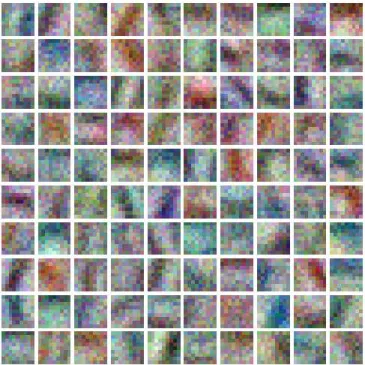
Figure 2.4 provides an example of the filters learned on the first convolutional layer of a network trained for traffic sign recognition, showing that this type of architecture is capable of learning interesting feature detectors, similar to edge detectors.

Figure 2.4: Sample feature maps learned by a convolution network for traffic sign recog-nition [36]

2.3.1 Convolutional layers

Convolutional layers have trainable filters (also called feature maps) that are applied across the entire input[37]. For each filter, each neuron is connected only to a subset of the neurons in the previous layer. In the case of 2D input (such as images), the filters define a small area (e.g. 5x5 or 8x8 pixels), and each neuron is connected only to the nearby neurons (in this area) in the previous layer. The weights are shared across neurons, leading the filters to learn frequent patterns that occur in any part of the image.

The definition for a 2D convolution layer is presented in Equation 2.17. It is the application of a discrete convolution of the inputs yl−1 _{with a filter} _ωl_{, adding a bias} _bl_,

(28)

y_rcl =σ( Fr X i=1 Fc X j=1 y₍l−_r₊1_i₋₁₎₍_c₊_j₋₁₎wl_ij +bl) (2.17) In this equation, yrcl is the output unit at {r, c}, Fr and Fc are the number of rows

and columns in the 2D filter,wl

ij is the value of the filter at position {i, j},y l−1

(r+i−1)(c+j−1)

is the value of input to this layer, at position{r+i−1, c+j−1}, andbl _{is the bias term.}

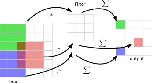
The forward propagation phase of a convolutional layer is illustrated in figure 2.5.

.* X .* X .* X Input Filter output

Figure 2.5: The forward propagation phase of a convolutional layer.

The equation above is defined for all possible applications of the filter, that is, for

r∈ {1, ..., Xr−Fr+ 1} and c∈ {1, ..., Xc−Fc+ 1}, whereXr and Xc are the number of

rows and columns in the input to this layer. The convolutional layer can either apply the filters for all possible inputs, or use a different strategy. Mainly to reduce computation time, instead of applying the filter for all possible{r, c}pairs, only the pairs with distance

sare used, which is called thestride. A strides = 1 is equivalent to apply the convolution for all possible pairs, as defined above.

The inspiration for convolutional layers originated from models of the mammal visual system. Modern research in the physiology of the visual system found it consistent with the processing mechanism of convolutional neural networks, at least for quick recognition of objects [13]. Although being a biological plausible model, the theoretical reasons for the success of convolutional networks are not yet fully understood. One hypothesis is

(29)

that the small fan-in of the neurons (i.e. the number or input connections to the neurons) helps the derivatives to propagate through many layers - instead of being diffused in a large number of input neurons.

2.3.2 Pooling layers

The pooling layers implement a non-linear downsampling function, in order to reduce dimensionality and capture small translation invariances. Equation 2.18 presents the formulation of one type of pooling layer, max-pooling:

y_rcl = max

i,j∈{0,1,...,m}y l−1

(r+i−1)(c+j−1) (2.18)

In this equation,yl

rcis the output for index{r, c},mis the size of the pooling area, and

y₍l−_r₊1_i₋₁₎₍_c₊_j₋₁₎ is the value of the input at the position {r+i−1, c+j−1}. Similarly for the convolutional layer described above, instead of generating all possible pairs of {i, j}, a stride s can be used. In particular, a stride s = 1 is equivalent to using all possible pooling windows, and a stride s = m is equivalent of using all non-overlapping pooling windows. Figure 2.6 illustrates a max-pooling layer with stride=1.

max

Input

output

Figure 2.6: The forward propagation phase of a pooling layer.

Scherer et al. [38] evaluated different pooling architectures, and note that the max-pooling layers obtained the best results. Pooling layers add robustness to the model, providing a small degree of translation invariance, since the unit activates independently on where the image feature is located within the pooling window [16]. Empirically, pooling has demonstrated to contribute to improved classification accuracy for object recognition [37].

(30)

2.3.3 Locally-connected layers

Locally-connected layers only connect neurons within a small window to the next layer, similarly to convolutional layers, but without sharing weights. The motivation for this type of layer is to achieve something similar to one of the benefits of convolutional layers: to reduce the fan-in of the neurons (the number of input connections to each neuron), enabling the derivatives to propagate through more layers instead of being diffused.

y_rcl =σ( m X i=1 m X j=1 W_ijl,rcy₍l−_r₊1_i₋₁₎₍_c₊_j₋₁₎) (2.19) Where: W_ijl,rc is the weight associated with layer l, producing the output unit r, c at position i, j, and y₍l−_r₊1_i₋₁₎₍_c₊_j₋₁₎ is the input at position (r+i−1),(c+j−1).

2.4 Combining Classifiers

We now provide an overview of a strategy used in the present work - the combination of multiple classifiers.

One strategy to increase the performance of a pattern recognition system is to, instead of relying on a single classifier, use a combination of multiple classifiers. This is particu-larly useful when the errors of different classifiers do not completely overlap - suggesting that these classifiers offer complementary information on the examples. Several strate-gies can be used for creating such classifiers, such as using different feature sets, different training sets, etc. [39].

Kittler et al. [39] provide a theoretical framework for combining classifiers, showing different assumptions (on the classifiers’ properties), under which common combination techniques can be derived. The equations for the two most used combination strategies are shown below, simplified for the case where the classes have equal priors:

The Product rule is defined in equation 2.20. It combines the classifiers under the assumption that they are conditionally independent.

(31)

assign Z →ωj if R Y i=1 p(xi|ωj) = m max k=1 R Y i=1 p(xi|ωk) (2.20)

In this equation, Z is the pattern being classified, ωk are the different classes, and

p(xi|ωk) is the probability assigned to classk by the classifier i.

The Sum rule is defined in equation 2.21. It combines the classifiers under the assumption that the classifiers will not deviate dramatically from the prior probabilities.

assign Z →ωj if R X i=1 p(xi|ωj) = m max k=1 R X i=1 p(xi|ωk) (2.21)

Similar to the equation above, Z is the pattern being classified, ωk are the different

classes, and p(xi|ωk) is the probability assigned to classk by the classifier i.

2.5 Transfer Learning

Transfer learning is a strategy that aims to improve the performance on a machine learning task by leveraging knowledge obtained from a different task. The intuition is: we expect that by learning one task we gain knowledge that could be used to learn similar tasks. For example, learning to recognize apples might help in recognizing pears, or learning to play the electronic organ may help learning the piano [40].

In a survey on transfer learning, Pan and Yang [40] use the following notations and definitions for transfer learning: A domain D consists of two components: a feature space X and a probability distribution P(X), where X ={x1, ..., xn} ∈ X. Given a

specific domain, D={X, P(X)}, a task consist of two components: a label spaceY and an objective predictive function f(.), denoted by T = {Y, f(.)}), which is not observed, but that can be learned from training data. The functionf(.) can then be used to predict

(32)

the corresponding label,f(x) of a new instancex. From a probabilistic perspective,f(x) can be written as P(y|x). In an example in the texture classification domain, we use a feature descriptor on the textures to generate the feature space X. A given training sample is denoted by X,X ∈ X, with associated label y, y∈ Y. A model is then trained on a dataset to learn the function f(.) (or P(y|x)).

With this notation, transfer learning can be defined as follows:

Definition 2.5.1 Given a source domain DS and learning task TS, a target domain DT

and learning task TT, transfer learning aims to help improve the learning of the target

predictive function fT(.) in DT using the knowledge in DS and TS, where DS 6= DT, or

TS 6=TT

To illustrate, we can use this definition for texture classification. We can apply transfer learning by using a source task from a different domain D, for example, using a different feature space X (with a different feature descriptor) or using a dataset with different marginal probabilitiesP(X) (i.e. textures that display different properties from the target task). We can also apply transfer learning if the task T is different: for example, using a source task that learns different labels Y or with different objective f(.).

2.5.1 Transfer Learning in Convolutional Neural Networks

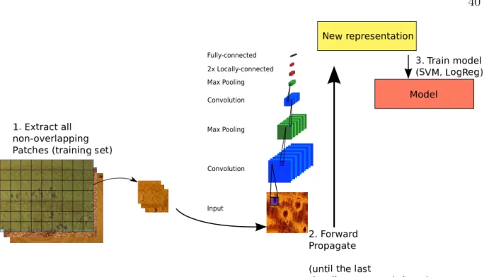
The architecture of state-of-the-art Convolutional Neural Networks (CNN) often contains a large number of parameters, such as the network of Krizhevsky et. al for the ImageNet dataset [26] with 60 million parameters. In this case, the weights are learned from a dataset containing 1.2 million high-resolution images for training. However, directly learning so many parameters from only a few thousand examples is problematic. Transfer learning can assist in this task, by using the internal representation learned from one task, and applying it to another task. As noted by Oquab et. al [41], a CNN can act as a generic extractor of mid-level representations, which can be pre-trained in a source task, and then re-used in other target tasks.

(33)

differ significantly between the source and target tasks. Oquab et. al [41] propose a simple method to cope with this problem, by training an adaptation layer (using the target dataset), after the convolutional layers are learned in the source task. This process is illustrated in Fig 2.7: first a convolutional neural network is trained in the source task (in their case the ImageNet dataset). The parameters learned by network (except for the last layer) are then transferred to the target task (which has a smaller dataset). To compensate for the different distribution of the images, two fully-connected layers are added to the network, and these two layers are then trained using the target dataset. Using this simple transfer learning procedure, Oquab et. al were able to achieve state-of-the-art results on the competitive Pascal VOC dataset.

(34)

CHAPTER 3 STATE-OF-THE-ART

This Chapter reviews the state-of-the-art for Deep Neural Networks applied to a classifica-tion task. Deep models were already successfully used in many domains, including several classification tasks [33], [42], [18], natural language processing [43], acoustic modelling in speech recognition[44] , among others. The present work is focused on texture classifica-tion, and therefore we limited the analysis for image recognition tasks. In particular, one object recognition problem was selected (CIFAR-10) for comparative analysis. The best published results on this dataset are compared, and their similarities are identified.

3.1 Deep learning review on the CIFAR-10 dataset

Deep learning has been a focus of recent research, and a large variety of models have been proposed in recent years [13]. To support the decisions on which strategies to pursue for texture classification, a survey was conducted on the top published results in an object recognition task: CIFAR-10 [17]. Several similarities were found in the models and methodologies used in these papers, which provided insights for the texture classification task. The detailed results of this analysis can be found below, and it is summarized in the next section.

Goodfellow et al. [45] achieved the best published result on the CIFAR-10 dataset. They used an architecture of three convolutional-layers (each followed by a max-pooling layer), followed by one fully-connected layer, and one fully-connected softmax layer. The key difference on this work is the usage of a new type of neuron, called Maxout, instead of using the sigmoid function. A single maxout neuron can approximate any convex func-tion, and in practice the maxout networks not only learn the relationships between hidden neurons, but also the activation function of each neuron. Their model also made usage of a regularization technique called dropout [46], which is described below. With this

(35)

archi-tecture, an accuracy of 90.65% was achieved in this 10-class classification problem. This result was achieved by augmenting the training dataset with translations and horizontal reflections, and using standard preprocessing techniques: Global contrast normalization, and ZCA whitening.

Snoek et al. [47] used the same architecture defined by Krizhevsky in the first tests with the CIFAR-10 dataset [17]. Considering the fact that deep networks have a significant number of hyperparameters (such as the number of layers, and the size of each layer), they developed a Bayesian Optimization procedure for tuning these hyperparameters. The net-work architecture is similar to the one used by Goodfellow, with two convolutional layers, but instead of the maxout neuron, Rectified Linear Units (RELUs) where used. Snoek et al. started training with the best hyperparameters obtained manually (by Krizhevsky), and used their method to fine-tune them. As a result, they were able to achieve 90.5% of accuracy on this task, compared to 82% of accuracy obtained by Krizhevsky. Again, the training dataset was augmented with translations and reflections to achieve this level of accuracy.

Ciresan et al. [18] proposed a method for image classification relying on multiple deep neural networks trained on the same data, but with different preprocessing techniques. The networks are trained separately, and then the results are combined, by averaging the outputs of the different networks. The architecture of the networks consisted of four convolutional layers, followed by a fully-connected layer, and a softmax layer. Training followed this procedure: At first, all images are preprocessed using multiple techniques, obtaining 5 different versions of each image - they used standard image processing tech-niques such as Histogram equalization, and Adaptive Histogram equalization. At the beginning of each epoch, each image in the dataset is randomly translated, scaled and rotated (i.e. the dataset is augmented). This updated dataset is then used to train the networks. During test, the images are pre-processed with the same techniques, and the results are combined by averaging the outputs of all networks. With this architecture, an accuracy of 88.79% was obtained.

(36)

called stochastic pooling. The most common pooling strategy, max-pooling, works by selecting only the largest value of the pooling window. In the proposed method, a proba-bility is assigned to each element in the window, where the larger values within the window are given higher probabilities. One of the values is then stochastically selected using these probabilities. At test time, the values of the window are averaged in a probabilistic form, by multiplying the values by their probability within the window. The network architec-ture contained three convolutional layers, each followed by stochastic pooling, and a local response normalization layer (which normalizes the pooling outputs at each location over a subset of neighboring feature maps). Lastly, a single fully-connected softmax layer is used to obtain the model predictions. With this architecture, an accuracy of 84.87% was obtained.

Hinton et al. [46] introduced a model regularization technique called dropout. The basic idea for dropout is that for each example (or mini-batch) of training, some of the neurons are deactivated (i.e. they are not used in the forward/back-propagation phases). In practice this is equivalent on training an ensemble of networks containing the set of all possible network configurations (i.e. all possible networks obtained by deactivating a given percentage of the neurons in each layer). At test time, the full network is used, which is equivalent to running the input in all possible network configurations, and averaging their result. The model for the CIFAR-10 dataset contained three convolutional layers, each followed by max-pooling and Local Response Normalization. A locally-connected layer is used after the convolutional layers, and a 50% dropout is used in this layer. The last layer is a softmax layer, which produces the model outputs. With this architecture, an accuracy of 84.40% was obtained.

3.1.1 Summary of the CIFAR-10 top results

Table 3.1 provides a summary of the papers reviewed above. The most important simi-larities among the models are the following:

(37)

2. No models used unsupervised pre-training

3. Best results used data augmentation (translation, rotation, scaling)

It is worth noting that none of top five results used unsupervised pre-training, in spite of the fact that such models, using RBMs and autoenconders, were fundamental for obtaining early successful results with deep learning. We can also see that the best results used techniques that expand (augment) the original datasets, such as translations and rotations.

(38)

26

90.65% [45] Deep Convolutional Neural Network with Maxout

- Global contrast nor-malization - ZCA whitening Yes: - Image translations - Horizontal Reflec-tions No CNN with:

- Convolutional maxout layers with max-pooling (x3)

- Fully connected maxout layer - Softmax layer

90.50% [47] Deep Convolutional Neural Network

Mean normalization Yes:

- Image translations - Horizontal Reflec-tions

No CNN with:

- Convolutional layer followed by max-pooling and local contrast normalization (x2)

- Two locally connected layers - Softmax layer

88.79% [18] MCDNN (Multi-column Deep Con-volutional Neural Network) Image processing: - Image Adjustment - Histogram equaliza-tion - Adaptive Histogram Equalization - Contrast Normaliza-tion Yes - Rotation±5◦ - Scaling±15% - Translation ±15%

No Several CNNs trained separately, and aver-aged in a MCDNN. CNNs are trained on data pre-processed using different techniques. - Used large number of wide layers (6 to 10 layers with hundreds of maps)

- Used convolutional layers, with max-pooling

84.87% [48] Deep Convolutional Neural Network

Mean normalization No No CNN with:

- Convolutional layer followed by stochas-tic pooling and local response normalization. (x3)

- Softmax layer 84.40% [46] Deep Convolutional

Neural Network with Dropout

Mean normalization No No CNN with:

- Convolutional layers followed by pooling and local response normalization.(x3)

- One locally-connected layer (where dropout of 50% is applied)

- Softmax layer Table 3.1: Comparison of top published results on the CIFAR-10 dataset

(39)

CHAPTER 4 METHODOLOGY

In this Chapter we propose a methodology to train Convolutional Neural Networks on texture classification problems. We start with a general definition on the learning process, and introduce the texture datasets that we use to evaluate the methodology. We then present our method for training the networks on texture problems, and the method we use to transfer learning between tasks.

From a high-level, the process to train and evaluate the models follows the standard method for pattern recognition problems. The objective is to use a machine learning algorithm to learn a classification model, using a training dataset. We can then use this model to classify new samples, with the expectation that the patterns learned by the model in the training set generalize for new data. This process is illustrated in Figure 4.1.

Machine Learning Algorithm

Figure 4.1: An overview of the Pattern Recognition process.

To evaluate the models, we use a held-out testing set to calculate the accuracy of the model, to verify how the model performs on unseen data:

Accuracy = # correct predictions

# samples in the testing set (4.1) For each dataset, the best architectures are validated using 3-fold cross-validation, that

(40)

is, the dataset is split three times (folds) into training, validation and testing. For each fold, a model is trained using the training and validation sets, and tested in the testing set. We then report the mean and standard deviation of the accuracy and compare them with the state-of-the-art in each dataset.

4.1 Texture datasets

A total of six texture datasets were selected to evaluate the method. These datasets were selected for two main reasons: they represent problems in different domains, and each dataset contain different challenges for pattern recognition. Below is a description of the selected datasets, with the different challenges that they pose. Examples of these datasets can be found in Appendix A

4.1.1 Forest Species datasets

The first dataset contains macroscopic images for forest species recognition: pictures of cross-section surfaces of the trees, obtained using a regular digital camera. This dataset consists in 41 classes, containing high-resolution (3264 x 2448) images for each class. The procedure used to collect the images, and details on the initial dataset (that contained 11 classes at the time) can be found in [49], and the full dataset in [50].

The second dataset contains microscopic images of forest species, obtained using a laboratory procedure. This dataset consists of 112 species, containing 20 images of res-olution 1024x768 for each class. Details on the dataset, including the procedure used to collect the images can be found in [51]. Examples of this dataset are presented in Figure A.2. It is worth noting that the colors on the images are not natural from the forest species, but a result of the laboratory procedure to produce contrast on the microscopic images. Therefore, the colors are not used for training the classifiers.

The main challenge on the two forest species datasets is the image size. Most successful deep network models rely on small image sizes (e.g. 64x64), and these datasets contain images that are much larger.

(41)

4.1.2 Writer identification

We consider two writer identification datasets. The first is the Brazilian Forensic Let-ter Database (BFL), containing 945 images from 315 wriLet-ters (3 images per wriLet-ter)[52]. Hanusiak et al. [53] introduced a method to create textures from this type of image, transforming it into a texture classification problem. This method was later explored in depth by Bertolini [8] in two datasets: The Brazilian Forensic Letter Database, and the IAM Database. The IAM Database was presented by Marti and Bunke[54] for offline handwritten recognition tasks. The dataset includes scanned handwritten forms produced by approximately 650 different writers. Samples of these datasets, and their associated texture can be found in Figures A.4 and A.5. To allow direct comparison with published results on these datasets, we use the same subsets of the data as Bertolini [8]. In partic-ular, we use 115 writers from the BFL dataset, and 240 writers from the IAM dataset. This large number of classes is the main challenge in these datasets.

4.1.3 Music genre classification

The Latin Music Dataset, introduced by Silla et al. [55] contains 3227 songs from 10 different Latin genres, and it was primarily built for the task of automatic music genre classification. Costa et al. [56] introduced a novel approach for this task, using spec-trograms: a visual representation of the songs. With this approach, a new dataset was constructed, with the images (spectrograms) of the songs, enabling the usage of classic texture classification techniques for this task.

The music genre dataset contains a property that distinguishes it from the other datasets: on the other datasets, the textures are more homogeneous, in the sense that patches from different parts of the image have similar characteristics. For this dataset, however, there are differences in both axis: The music change its structure over time (X axis), and different patterns are expected on the frequency domain (Y axis). This suggest that convolutions can be less effective in this dataset, as patterns that are useful for one part of the image may not be useful for other parts. The challenge is to test if convolutions obtain good results in spite of these differences, or adapt the methodology to use a zoning

(42)

division, as described in the work by Costa et al. [56] and illustrated in figure 4.2.

Figure 4.2: The zoning methodology used by Costa [56].

4.1.4 Brodatz texture classification

The Brodatz album is a classical texture database, dating back to 1966, and it is widely used for texture analysis. [57]. This dataset is composed of 112 textures, with a single 640x640 image per each texture. In order to standardize the usage of this dataset for texture classification, Valkealahti [58] introduced the Brodatz-32 dataset, a subset of 32 textures from the Brodatz album, with 64 images per class (64x64 pixels in size), containing patches of the original images, together with rotated and scaled versions of them (see Figure A.6).

The challenge with the Brodatz dataset is the lower number of samples per image. In the original Brodatz dataset, only a single image per texture is available (640x640). Since it is common for Convolutional Networks to have large number of parameters, this type of network usually require large datasets to be able to learn the patterns from the data.

(43)

4.1.5 Summary of the datasets

Table 4.1 summarizes the properties of the datasets used in this research, showing the different challenges (in terms of number of classes, database size, etc.) as mentioned in the previous sections.

The last column of the table counts the number of bytes used to represent the images in a bitmap format (i.e. 1 byte per pixel for grayscale images, 3 bytes per pixel for color images), to give a sense on the amount of information available for the classifier in each dataset. Dataset Num. Classes Num. Samples per Class Total Num. of Samples

Image size Number of bytes Forest species (Macroscopic) 41 37 ∼99 2942 3264 x 2448 (color) ∼65.7 GB Forest species (Microscopic) 112 20 2240 1024 x 768 ∼1.6 GB Music Genre Classification 10 90 900 800 x 513 ∼352 MB Write identifica-tion (BFL) 115 27 3105 256 x 256 ∼194 MB Write identifica-tion (IAM) 240 18 4320 128 x 256 ∼135 MB Brodatz-32 Tex-ture classification 32 64 2048 64 x 64 ∼8 MB

Table 4.1: Summary of the properties of the datasets

4.2 Training Method for CNNs on Texture Datasets

The proposed method for training CNNs on texture datasets is outlined below. The next sections describe the steps in further detail, and provide a rationale for the decisions.

1. Resize the images from the dataset

2. Split the dataset into training, validation and testing 3. Extract patches from the images

(44)

4. Train a convolutional neural network on the patches using the training and valida-tion sets

5. Test the network on the test patches

6. Combine the patches to report results on the whole test images

4.2.1 Image resize and patch extraction

Most tasks that were successfully modeled with deep neural networks usually involve small inputs (e.g 32x32 pixels up to 108x108 pixels). Networks with larger input sizes contain more trainable weights requiring significant more computing power to train, and also requiring more data to prevent overfitting.

In the case of texture classification, it is common to have access to high-resolution texture images, and therefore we need to methods that can explore larger inputs. Instead of simply training larger networks, we explore the hypothesis that we can classify a texture image with only a small part of it, and train a network not on the full texture images, but on patches of the images. This assists in reducing the size of the input to the neural network, and also allows us to combine, for a given image, different predictions made using patches from different parts of the image.

Besides the size of the input to the neural network, another important aspect is the size of the filter (feature map) for the first convolutional layer. The first layer is responsible for the first level of feature extractors, which are closely related to local features in the image. Therefore, the filter size must be adequate for the dataset images (and vice-versa), in the sense that relevant visual cues should be present in image patches of the size of the filter. Considering this hypothesis, we first resize the images so that relevant visual cues are found within windows of fixed filter sizes. We consider different filter sizes for the first layer following the results from Coates et al. [59], that investigated the impact of filter sizes in classification. Coates et al. empirically demonstrated that the best filter sizes are between 5x5 and 8x8. The usage of larger filter sizes would require significantly larger amounts of data to improve accuracy.

(45)

Besides this intuitive approach for choosing the filter size and the factor to resize the images, we also explore a more systematic approach, considering both as hyperparameters of the network, and optimizing them.

4.2.2 CNN architecture and training

The architecture of the neural networks are based on the best results on the CIFAR dataset (as reviewed in Chapter 3). In particular, we use multiple convolutional layers (each followed by max-pooling layers), followed by multiple non-convolutional layers, ending with a softmax layer. This architecture is illustrated in Figure 4.3

Convolution Convolution Max Pooling Max Pooling 2x Locally-connected Fully-connected Input

Figure 4.3: The Deep Convolutional Neural Network architecture. This architecture consists of the following layers, with the following parameters: 1. Input layer: the parameters are dependent on the image resolution and the number

of channels of the dataset;

2. Two combinations of convolutional and pooling layers: each convolutional layer has 64 filters, with a filter size defined for each problem, and stride set to 1. The pooling

(46)

layers consist of windows with size 3x3 and stride 2;

3. Two locally-connected layers: 32 filters of size 3x3 and stride 1;

4. Fully-connected output layer: dependent on the number of classes of the problem. The network has a high number of hyperparameters, such as the number of layers, the number of neurons in each layer, and different parameters in each layer’s configura-tion. In the present work we do not optimize all these hyperparameters. Instead, we started with network configurations that achieved state-of-the-art results on the CIFAR dataset, as described in Chapter 3, and performed tests in one of the texture datasets to select an architecture suitable for texture classification. We fixed the majority of the hyperparameters with this approach, we left the following hyperparameters for tuning:

• Patch Size: The size of the input layer in the CNN (cropped from the input image)

• Filter Size: The size of the filter in the first convolutional layer

• Image size (Resize factor): The size of the image (before extracting its patches), resized from the original dataset. This is a parameter from our training strategy, not a parameter for the Convolutional Network. During initial tests, we found that this parameter is correlated with the Filter size, impacting the network’s performance. For example, when the input image is large and does not contain relevant visual cues in a small area (e.g. 5x5 pixels) it requires larger filters to achieve good performance. To explore the impact of the image sizes together with the filter sizes, we consider both as hyperparameters to be optimized.

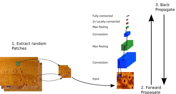
The training algorithm is similar to the Stochastic Gradient Descent algorithm (Al-gorithm 1) described in Chapter 2. The key difference is that the network is trained on random patches of the image - that is, for each epoch, a random patch is extracted for each image. We found that this strategy helps to prevent the model from overfitting the training set, while allowing training of a network with a large number of parameters. This procedure is defined in Algorithm 2 and illustrated in Figure 4.4.

(47)

Algorithm 2Training with Random Patches

Require: dataset, patchsize, batch size, learning rate, momentum factor

repeat

datasetepoch ← empty list

for each image in dataset do

Insert(datasetepoch, Random Image Crop(image, patchsize))

end for

numBatches← size(dataset) / batch size

for batch ←0 to numBatchesdo

datasetbatch ← datasetepoch[batch * batch size : (batch+1) * batch size -1]

model state ← ForwardProp(model, datasetbatch.X)

gradients ← BackProp(model state, datasetbatch.Y)

ApplyGradients(model, gradients, learning rate, momentum factor)

end for

until Convergence Criteria()

Here, Random Image Crop is a function that, given an image and a desired patch-Size, returns a random patch of size (patchSize x patchSize). ForwardProp and Back-Prop are the forward-propagation and back-propagation phases of the CNN training, as defined in Chapter 2. ApplyGradientsupdates the weights using the gradients (deriva-tives), the learning rate and applying momentum. We considered different termination criteria, and good results were obtained by setting a maximum number of iterations with-out improvement in the error function.

We train the Convolutional Neural Networks on a Tesla C2050 GPU, using the cuda-convnet library1_.

4.2.3 Combining Patches for testing

During training, the patches extracted from the images are classified individually, to cal-culate the error function and the gradients. During test, the different predictions on each

(48)

2. Forward Propagate 3. Back Propagate 1. Extract random Patches Convolution Convolution Max Pooling Max Pooling 2x Locally-connected Fully-connected Input

Figure 4.4: The training procedure using random patches

patch that compose an image need to be combined. For each patch, the model predicts the a posteriori probability of each class given the patch image. These probabilities are combined following the classifier combination strategies from Kittler et al. [39], reviewed in Chapter 2.

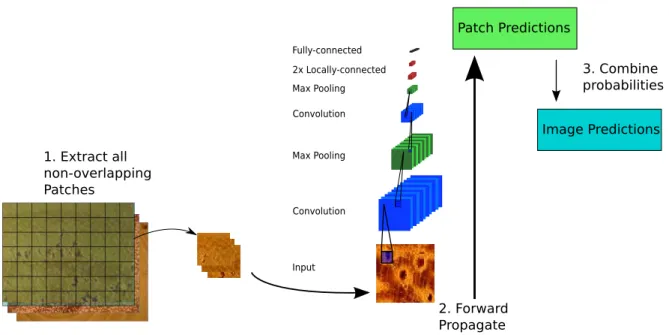
In the present work, we made the decision to use the set of all non-overlapping patches from the image during test (called here Grid Patches). For each image, we extract a list of patches, classify them all, and combine the probabilities from all patches of the image. This procedure is described in Algorithm 3 and illustrated in Figure 4.5.

An analysis of deep neural networks for texture classification

LUIZ GUSTAVO HAFEMANN

AN ANALYSIS OF DEEP NEURAL NETWORKS FOR

TEXTURE CLASSIFICATION

AN ANALYSIS OF DEEP NEURAL NETWORKS FOR

TEXTURE CLASSIFICATION

ACKNOWLEDGMENTS

CONTENTS

LIST OF FIGURES

LIST OF TABLES

RESUMO

ABSTRACT

CHAPTER 1

INTRODUCTION

1.1

Motivation

1.2

Challenges

1.3

Objectives

1.4

Contributions

CHAPTER 2

THEORETICAL BACKGROUND

2.1

Artificial Neural Networks

2.1.1

Artificial Neuron

2.1.2

Multi-layer Neural Networks

2.1.2.1

Forward Propagation

2.1.2.2

Training Objective

2.1.2.3

Backpropagation

2.1.2.4

Training algorithm

2.2

Training Deep Neural Networks

2.3

Convolutional Neural Networks

2.3.1

Convolutional layers

2.3.2

Pooling layers

2.3.3

Locally-connected layers

2.4

Combining Classifiers

2.5

Transfer Learning

2.5.1

Transfer Learning in Convolutional Neural Networks

CHAPTER 3

STATE-OF-THE-ART

3.1

Deep learning review on the CIFAR-10 dataset

3.1.1

Summary of the CIFAR-10 top results

CHAPTER 4

METHODOLOGY

4.1

Texture datasets

4.1.1

Forest Species datasets

4.1.2

Writer identification

4.1.3

Music genre classification

4.1.4

Brodatz texture classification

4.1.5

Summary of the datasets

4.2

Training Method for CNNs on Texture Datasets

4.2.1

Image resize and patch extraction

4.2.2

CNN architecture and training