Estimating the uncertainty of areal precipitation using data assimilation

precipitation using data assimilation

Article

Published Version

Creative Commons: Attribution 4.0 (CC-BY)

Open Access

Merker, C., Geppert, G., Clemens, M. and Ament, F. (2019)

Estimating the uncertainty of areal precipitation using data

assimilation. Tellus A: Dynamic Meteorology and

Oceanography, 71 (1). 1606666. ISSN 1600-0870 doi:

https://doi.org/10.1080/16000870.2019.1606666 Available at

http://centaur.reading.ac.uk/88694/

It is advisable to refer to the publisher’s version if you intend to cite from the

work. See

Guidance on citing

.

To link to this article DOI: http://dx.doi.org/10.1080/16000870.2019.1606666

Publisher: Taylor & Francis

All outputs in CentAUR are protected by Intellectual Property Rights law,

including copyright law. Copyright and IPR is retained by the creators or other

copyright holders. Terms and conditions for use of this material are defined in

the

End User Agreement

.

www.reading.ac.uk/centaur

CentAUR

Central Archive at the University of Reading

Reading’s research outputs online

Full Terms & Conditions of access and use can be found at

https://www.tandfonline.com/action/journalInformation?journalCode=zela20

ISSN: (Print) 1600-0870 (Online) Journal homepage: https://www.tandfonline.com/loi/zela20

Estimating the uncertainty of areal precipitation

using data assimilation

C. Merker, G. Geppert, M. Clemens & F. Ament

To cite this article:

C. Merker, G. Geppert, M. Clemens & F. Ament (2019) Estimating the

uncertainty of areal precipitation using data assimilation, Tellus A: Dynamic Meteorology and

Oceanography, 71:1, 1606666, DOI: 10.1080/16000870.2019.1606666

To link to this article:

https://doi.org/10.1080/16000870.2019.1606666

© 2019 The Author(s). Published by Informa UK Limited, trading as Taylor & Francis Group

Published online: 07 May 2019.

Submit your article to this journal

Article views: 557

View related articles

Estimating the uncertainty of areal precipitation using

data assimilation

By

C. MERKER

, G. GEPPERT

, M. CLEMENS

, and F. AMENT

,

Universit

€

at Hamburg,

Hamburg, Germany;

Department of Meteorology, University of Reading, UK;

National Centre for

Earth Observation, University of Reading, UK;

Max Planck Institute for Meteorology,

Hamburg, Germany

(Manuscript received 2 February 2018; in final form 04 April 2019)

ABSTRACT

We present a method to estimate spatially and temporally variable uncertainty of areal precipitation data. The aim of the method is to merge measurements from different sources, remote sensing and in situ, into a combined precipitation product and to provide an associated dynamic uncertainty estimate. This estimate should provide an accurate representation of uncertainty both in time and space, an adjustment to additional observations merged into the product through data assimilation, and flow dependency. Such a detailed uncertainty description is important for example to generate precipitation ensembles for probabilistic hydrological modelling or to specify accurate error covariances when using precipitation observations for data assimilation into numerical weather prediction models. The presented method uses the Local Ensemble Transform Kalman Filter and an ensemble nowcasting model. The model provides information about the precipitation displacement over time and is continuously updated by assimilation of observations. In this way, the precipitation product and its uncertainty estimate provided by the nowcasting ensemble evolve consistently in time and become flow-dependent. The method is evaluated in a proof of concept study focusing on weather radar data of four precipitation events. The study demonstrates that the dynamic areal uncertainty estimate outperforms a constant benchmark uncertainty value in all cases for one of the evaluated scores, and in half the number of cases for the other score. Thus, the flow dependency introduced by the coupling of data assimilation and nowcasting enables a more accurate spatial and temporal distribution of uncertainty. The mixed results achieved in the second score point out the importance of a good probabilistic nowcasting scheme for the performance of the method.

Keywords: data assimilation, precipitation measurements, uncertainty estimate, rain radar, nowcasting

1. Introduction

Precipitation information with an accurate uncertainty estimate is highly relevant for research areas with special interest in areal precipitation information. The uncer-tainty information is needed for example to generate precipitation ensembles as input for probabilistic hydro-logical modelling (e.g. Krajewski and Ciach, 2006; Germann et al., 2009; Rico-Ramirez et al., 2015; Park et al., 2016) or nowcasting (e.g. Atencia and Zawadzki,

2015; Dai et al.,2015). Furthermore, precipitation obser-vations are a valuable source of information for data

assimilation in numerical weather prediction (e.g. Dowell et al.,2011; Chang et al.,2014; Bick et al.,2016). Recent studies stress the importance of correctly specifying errors in this context (e.g. Waller et al.,2016,2017).

To assess the reliability of any observation, it is crucial to know its uncertainty. For precipitation observations, accurate measurements as well as a reliable estimate of their uncertainty are an ongoing topic of research. Observations from weather radars are of particular inter-est because they provide valuable areal precipitation information with high spatial and temporal resolution, in contrast to in situ observations. However, radar measure-ments are affected by numerous sources of error that diminish the accuracy of the provided precipitation quan-tification, e.g. calibration errors, noise, interferences, clut-ter, and attenuation. Despite the use of correction

Corresponding author. e-mail: [email protected] †_{Present address: Meteoswiss, Zurich, Switzerland€}

‡_{Present address: Deutscher Wetterdienst, Offenbach, Germany} This article has been republished with minor changes. These changes do not impact the academic content of the article.

Tellus A: 2019.#2019 The Author(s). Published by Informa UK Limited, trading as Taylor & Francis Group.

This is an Open Access article distributed under the terms of the Creative Commons Attribution License (http://creativecommons.org/licenses/by-nc/4.0/), which permits unrestricted non-commercial use, distribution, and reproduction in any medium, provided the original work is properly cited.

Citation: Tellus A: 2019,71, 1606666,https://doi.org/10.1080/16000870.2019.1606666

1

Tellus

DYANAMIC METEOROLOGY AND OCEANOGRAPHY

algorithms and filters on radar measurements, residual error remains inherent to the data. In addition, the esti-mation of rainfall intensity from radar data requires a relation between measured reflectivity and rain rate which is empirical and uncertain. Therefore, accurate rainfall precipitation quantification is not possible with radar measurements only. An extensive review of uncertainty sources in single polarisation radar measurements is given in Villarini and Krajewski (2010) and citations therein.

Improvements in the precipitation estimate are achieved by combining measurements from different sources, e.g. radar and rain gauge data, to take advantage of as much information as possible. Since no observation is error-free, they must be weighted with their respective uncertainty in order to obtain a statistically sound combined precipitation product. Many studies investigate the statistical combination of precipitation data. They rely on computing the optimal estimate of precipitation by minimising its error variance. The majority of the applied techniques focus on a static, i.e. time-independent, merging approach, where precipitation measurements are combined for every available time step independently. Most merging approaches use kriging or cokriging schemes to spatially merge radar and rain gauge data (e.g. Krajewski,1987; Creutin et al.,1988; Haberlandt,

2007; Berndt et al., 2014). Kriging methods acknowledge the fact that precipitation observation errors are spatially correlated by the specification of variograms. These vario-grams are modelled based on theoretical considerations, and do not consider the temporal structure of the errors. Less commonly used are variational data assimilation methods that describe the correlation between observation errors through covariance matrices. These methods can easily be extended to include further observations. For example, Bianchi et al. (2013) use a variational approach to estimate precipitation from radar, gauge and microwave link data.

Some studies additionally take into account the tem-poral correlation of precipitation measurement errors while merging radar and gauge data. The temporal struc-ture of the errors can be considered either by modelling spatio-temporal variograms in the kriging approach (e.g. Sideris et al., 2014, Pulkkinen et al., 2016) or by using Kalman filtering that combines knowledge on error var-iances from previous time steps for the current weighting of observations (e.g. Smith and Krajewski, 1991; Chumchean et al.,2006). The latter approach is also used by Grum et al. (2005) with the addition of microwave link data. Even though these methods consider temporal error structures in the merging process, the continuous evolution of the precipitation system is not represented.

Very few studies include a forecast model that evolves the system’s state to take advantage of previous know-ledge of the system. The coupling of a forecasting model can be done using Kalman filtering or variational data

assimilation methods. In addition to the merging of observations, the forecasting component allows for the extrapolation of information to data-void regions. Advection is commonly used as an approximation for the evolution of precipitation systems. Zinevich et al. (2009) and Mercier et al. (2015) present frameworks to estimate areal precipitation from microwave and television satellite links, respectively. Fielding et al. (2014) retrieve three-dimensional cloud properties from cloud radar and radi-ance observations. These studies integrate the temporal evolution of the system into the statistical merging of observations with a focus on retrieving the optimal com-bined estimate of the system’s state. However, they do not focus on an assessment of the uncertainty associated with the resulting precipitation field.

Considering radar precipitation data, uncertainty esti-mation is extensively studied outside the context of com-bined precipitation products. Numerous studies address the quantification of precipitation data uncertainty to overcome the deterministic view on radar precipitation measurements. The basis for the description of areal pre-cipitation measurement errors mostly is an empirical, statistical study of radar and reference surface measure-ments. Some methods only provide static information (Krajewski and Ciach, 2006), while more recent approaches also allow for the description of the spatial and temporal structure of the errors through the descrip-tion of the error covariance (e.g. Ciach et al., 2007; Germann et al.,2009; Villarini and Krajewski, 2009; Dai et al., 2014). Such spatial uncertainty description allows for a probabilistic assessment of precipitation information suitable for applications. However, the resulting error description is neither dynamical nor flow-dependent.

Here, we present a method that connects both aspects: pre-cipitation data merging and probabilistic uncertainty assess-ment. The method allows for the combination of precipitation observations considering their respective uncer-tainty and takes advantage of the additional information pro-vided by the temporal evolution of the system. At the same time, the method yields an areal uncertainty estimate for the resulting precipitation product. Because of the included tem-poral evolution, the uncertainty estimate is variable both in space and time and is flow-dependent. Thus, this method aims at providing both an accurate precipitation product and an improved areal and dynamical uncertainty estimate.

Our approach uses data assimilation as a tool to merge precipitation observations. This study considers radar data with different spatial resolution, but the method can be extended to incorporate any additional source of pre-cipitation observation. Data assimilation techniques allow for statistically combining all available information con-sidering its uncertainty within a temporal evolution model. The Local Ensemble Transform Kalman Filter

(LETKF, Bishop et al., 2001; Ott et al., 2004; Hunt et al.,2007) used here is especially suited for the purpose of this study. Its main feature is the description of uncer-tainty through covariance matrices estimated by an ensemble approach. The additional use of localisation in the LETKF reduces the required number of ensemble members to adequately represent the covariances. Through both the use of an ensemble and the localisa-tion, the LETKF is computationally much more afford-able for our problem size than the standard Kalman filter approach (Kalman, 1960; Kalman and Bucy, 1961; Talagrand, 1997). Furthermore, the ensemble approach can handle non-linear forecast models. In the presented setup, the LETKF is coupled to an ensemble nowcasting model to provide information about the displacement of precipitation over time.

The added value of the presented method is demon-strated in four experiments with observations from an

X-band radar network. The method’s functioning, including the LETKF and the coupled nowcasting scheme, is pre-sented in Section 2, Section 3 briefly presents the data. The performed experiments are introduced in Section 4 and the obtained precipitation product is evaluated in Section 5.

2. Method

The combination of a data assimilation method with a nowcasting method introduces flow dependency to the areal uncertainty estimate, as known uncertainty is propagated in time and space. In this way, the method yields a situation-dependent uncertainty estimate whose structure follows the evolution of the system. The overall functioning of the method is outlined in the flowchart in

Fig. 1. The ensemble data assimilation cycle allows for obtaining a combined precipitation product and a

Fig. 1. Flowchart illustrating the data assimilation cycle of the method for uncertainty estimation. Combined precipitation product and uncertainty estimate are obtained from the analysis ensemble mean and spread, respectively.

corresponding uncertainty estimate from the ensemble mean and spread, respectively. The data assimilation scheme (LETKF) and the coupled nowcasting scheme are introduced in the following.

2.1. The LETKF

Data assimilation aims at combining different sources of information about an observed system, weighted by their respective uncertainty, in order to get the best possible estimate of the system’s true state. The data assimilation method used here is the LETKF that allows to work with an ensemble of moderate size through a localisation approach. It was first introduced by Hunt et al. (2007) based on previous work by Bishop et al. (2001) and Ott et al. (2004). The complete set of LETKF equations (see Hunt et al.,2007for a complete derivation), consisting of the analysis and forecast steps, are given as

Analysis: ^xa_k ¼x^bkþKk yokHkx^bk h i Za k ¼ZbkTLETKFk TLETKF k ¼Ck½InþDk1=2CTk xa k;i ¼x^ a kþ ffiffiffiffiffiffiffiffi l1 p Za k;i Forecast:xb_kþ1;i ¼Mxa_k;i with Kk ¼P~ b kHTk HkP~ b kHTkþRk h i1 and Za_k;b ¼ ffiffiffiffiffiffiffiffi1 l1 p xak;;b1x^ a;b k x a;b k;2x^ a;b k . . .x a;b k;lx^ a;b k ; (1) where Ck is the matrix of eigenvectors of ZbT

k H T kR

1

k HkZbk and Dk is a diagonal matrix with the corresponding eigenvalues. In order to get the analysis ensemble mean after the update, ^xak; the background

ensemble mean before the update, ^xbk; is corrected by a term formed of the gain matrix Kk and the innovation vector yo_kHkx^bk:The gain matrix Kk weights the infor-mation by taking into account the Gaussian observation and background model error covariance matrices,Rk and

~

Pbk;respectively. In the context of the LETKF,P~ b k is the sample covariance matrix obtained from the background ensemble perturbations, i.e. the deviations from the ensemble mean. The innovation vector holds the differen-ces between observations yo_k used for assimilation in the considered time step and the ensemble meanx^bkin obser-vation space. Hk is the observation operator mapping model variables to observation space for comparison. The scaled analysis ensemble perturbations Za_k are obtained from the background ensemble perturbationsZb_k and the transformation matrixTLETKFk :The derivation of TLETKF

k is comprehensively described in Hunt et al. (2007) and Livings et al. (2008). The analysis model ensemble after the update, xa_k;i with i¼1;. . .;l denoting the member, is obtained by adding the new analysis per-turbations, Zak;i;to the analysis ensemble mean. The per-formed steps are summarised in Fig. 1. The analysis is performed independently at each grid point to increase the degree of freedom of the analysis otherwise limited by the low-rank approximation of the ensemble. After per-forming the analysis step, the data assimilation cycle is completed by running a forecast until the next update time step. The forecast is performed by applying the fore-cast model M on every model ensemble member separ-ately, which allows for non-linear forecast processes. In the case of the presented study, the system to be described is areal precipitation information, the forecast model used to predict the areal precipitation evolution is

Fig. 2. Example of input precipitation images for template-matching for the 3 July 2013. (a) 15:23:00 UTC and (b) 15:26:00 UTC and resulting displacement vector field, thinned out to every tenth pixel in each direction in this representation.

the ensemble nowcasting scheme introduced in the follow-ing section.

2.2. Ensemble nowcasting

The nowcasting scheme used for the proof of concept study is a simple approach based on template-matching between time-lagged precipitation images. The original algorithm, the Automated Precipitation Extrapolator (APEX), was developed by van Horne (2003) and is adopted here with some modifications.

The algorithm considers two consecutive precipitation images and computes an estimate of the precipitation dis-placement from the first to the second image. A correl-ation is calculated between the second image and spatially shifted versions of the first image. The spatial shift is performed in every direction and with different amplitudes and the shift yielding the best correlation allows for estimating the displacement of the precipitation structure between both images. The resulting displace-ment vector field indicates the precipitation motion direc-tion and speed, as demonstrated inFig. 2. The computed displacement between both images is then used to extrapolate the precipitation structure to its position at future time steps.

The complete displacement vector field (one vector per pixel in the precipitation field) is used to compute the precipitation forecast. Displacement vector lengths are scaled to the desired forecast time step and the future position of the precipitation field in the second image is predicted accordingly. In order to get a smooth,

continuous precipitation field after the advection, a 33 window of pixels around each pixel is shifted to its new position. If more than one precipitation value is attrib-uted to a pixel of the forecasted precipitation field, values are averaged, as illustrated in Fig. 3. The APEX algo-rithm computes a hierarchical correlation analysis consid-ering first the whole domain of the images and then smaller subregions. Due to the computation of local dis-placement vectors at each pixel covered with precipita-tion, some divergence and rotation is allowed in the vector field. The original precipitation can therefore be distorted during the forecasting process, accounting for some internal variability in the structure of the precipita-tion field. Precipitaprecipita-tion intensity can change compared to the initial field due to the averaging in the forecasting step, but for the sake of simplicity no cell growth and decay model is integrated in the nowcasting scheme. The prediction of the internal evolution of precipitation sys-tems is complex. More elaborated probabilistic nowcast-ing methods which explicitly try to account for the uncertainty arising from growth and decay of precipita-tion cells exist (e.g. Bowler et al., 2006; Atencia and Zawadzki, 2014). In a further step subsequent to this study, it is possible to extend the presented nowcasting method to include this aspect, or even to replace it with a method of choice.

To create an ensemble forecast from the deterministic nowcasting scheme, we generate an ensemble of displace-ment vector fields from the deterministic field by ran-domly perturbing its x- and y-components. The perturbations are multiplicative and drawn from a

Fig. 3. Schematic representation of the forecasting step for three pixels, exemplary. 33 windows of pixels (initial position left) are shifted according to the local motion vectors calculated for the middle pixel. If these pixel windows overlap in the forecast (new position right), pixel values (precipitation intensity or motion velocity) are averaged to get the forecasted field. In this example, light grey pixels are averages over two values, dark grey over three values.

Gaussian distribution with mean 1 and variance 0.4. The aim of the ensemble generation process is to produce a smooth perturbation of the displacement vector field. Therefore, the random noise from which the perturba-tions are built must be spatially correlated to avoid fuzzy and inconsistent displacement vectors. To create the pat-tern of the spatial correlation, areas with high wind speeds are assumed to behave similarly, i.e. perturbations applied to vectors with large displacement magnitude are strongly correlated. In this way, the structure of the pre-cipitation field is reflected in the correlation of the applied random noise. The ensemble size for this study is 50 (results with smaller or larger ensemble size do not dif-fer qualitatively from the results presented here). The detailed procedure as well as a sensitivity study for the chosen variance of the Gaussian noise is described in Merker (2017).

3. Data

This study uses radar reflectivity data from a research radar network. Both the network and the data are thor-oughly described in Lengfeld et al. (2014), together with all applied post-processing algorithms (including calibra-tion and attenuacalibra-tion correccalibra-tion). The radar network com-prises four X-band radars with a range of 20 km. Data are available as single radar product with 1 azimuthal, 60 m radial and 30 s temporal resolution, and in the form of a network composite product. The composite data have the same temporal resolution as the single radar data and a spatial resolution of 250 m250 m on a quasi-Cartesian grid, with a total of 297213 pixels. The quasi-Cartesian grid is computed on rotated spherical

coordinates with rotated pole at 36.0625 E, 170.415 S (refer to Lengfeld et al.,2014for details on the composite generation). The location of the four radars, the domain covered by the radar composite and the position of add-itional micro rain radars (MRR) and gauges for reference purposes are indicated inFig. 4.

The Cartesian composite radar data are used to initial-ise the nowcasting method presented in Section 2.2. For simplicity and because the coordinate system is irrelevant to the presented study, all figures will be presented in rotated coordinates.

Observations considered for assimilation in this study are taken from single radar measurements (X-band radar MOD in Lengfeld et al., 2014, lower centre circle inFig. 4). Observations are thinned to a 5000 m5000 m grid (2020 grid boxes in the nowcasting domain) within the reach of X-band radar MOD, resulting in 52 observation locations (Fig. 5). Each reflectivity observation is selected from the radar’s polar grid by using the nearest neigh-bour method. These observations are illustrative for any additional information about the system and could be extended by e.g. data from a rain gauge network in a fur-ther development. In the setup of this study, observations are treated similarly to radar data, which is most com-monly thinned or superobbed on a spaced, regular grid for direct radar data assimilation. This is done to reduce computational costs and representativity disparity and especially to avoid correlation of observation errors (e.g. Alpert and Kumar, 2007; Simonin et al., 2014; Bick et al.,2016; Waller et al.,2016). In addition, thinning of dense observations is needed to obtain an analysis ensem-ble not completely dominated by the amount of observed values, and to prevent collapsing of the ensemble spread.

Fig. 4. Map of the radar network. X-band radar locations and maximum range in black, MRR locations in orange. X-band radars and associated MRRs are installed at BKM, HWT, MOD and QNS sites. Three MRRs are installed between X-band radars, at sites WST, MST, and OST, from west to east respectively, together with reference rain gauges.

Ground observations are not used here to avoid issues induced by point-to-area differences and the empirical relation between precipitation intensity and radar reflect-ivity. Both would add additional uncertainty to the study and increase the complexity of results to a level that is beyond the scope of the intended proof of concept.

Observation errors on the thinned 5000 m5000 m grid are assumed to be uncorrelated and with constant error variance. This is a simplifying assumption, espe-cially for radar data. The estimation of the full radar observation error statistics is a complex and ongoing topic of research (e.g. Xu et al., 2007; Berenguer and Zawadzki,2008; Waller et al.,2016). Recent studies show the benefits of more sophisticated error models, which allow for less thinning or superobbing of the data and can significantly improve the quality of the analysis as shown for example in Jacques and Zawadzki (2014,

2015). However, the use of uncorrelated error statistics still is a state-of-the-art procedure (e.g. Chung et al.,

2009; Simonin et al.,2014; Bick et al.,2016) and will also be applied here. The error variance of the radar data is estimated by comparing data from the network presented in Lengfeld et al. (2014) to reference measurements from MRR in order to get an error variance specific to the radar data used. The error variance is found to be 11.32 dB2_.

We focus on reflectivity data to avoid additional uncertainty coming from the empirical conversion from reflectivity to rain rate. The logarithmic reflectivity unit dBZis used throughout the study. For reference, a differ-ence of 1 dB translates approximately to a factor 1.25, and 2 dB to a factor 2 difference in non-logarithmic

reflectivity Z. For rain rate in mm h–1, these differences correspond to roughly a factor of 1.15 and 1.54, respect-ively. Following the example of Bick et al. (2016), the‘no rain’ value is set to 5 dBZ, approximately 0.07 mm h–1_,

and all reflectivity data are thresholded accordingly throughout the study.

4. Experiments

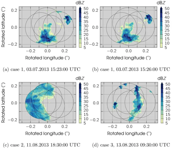
To assess the uncertainty estimate obtained by the method introduced inSection 2, we run coupled nowcast-ing-assimilation experiments using reflectivity data pre-sented in Section 3. The experiment setup and the detailed evaluation of the method in the following Section 5is first presented based on a precipitation event monitored by the radar network on 3 July 2013 between 15:30:00 UTC and 16:00:00 UTC (case 1), in which a non-stratiform cell passes through the radar network area. Thereafter, results from three additional precipita-tion events are included in the evaluaprecipita-tion to cover rele-vant regimes. Stratiform rain dominates on the 11 August 2013 (18:30:00 UTC–19:00:00 UTC, case 2), convective precipitation characterise the event on the 13 August 2013 (09:30:00 UTC–10:00:00 UTC, case 3) and the last case on the 17 August 2013 (03:30:00 UTC–04:00:00 UTC, case 4) features a frontal passage. An impression of these precipitation events is given inFig. 6.

As presented in Section 3, the ensemble forecast for the data assimilation experiment is initialised with radar composite data. Considering the first case of the study, forecast start is 15:26:00 UTC. The displacement vector field for the forecast is computed between composite

Fig. 5. Locations of thinned precipitation observations created for assimilation from data of the X-band radar at MOD site (Lengfeld et al.,2014) on a 5000 m5000 m grid (dots) and locations for verification on a 5000 m5000 m grid shifted by 2500 m north and east (crosses).

Fig. 6. X-band radar network composite reflectivity data (Lengfeld et al.,2014) for the four cases presented in the study: Case 1 on the 3 July 2013 15:23:00 UTC (a) and 15:26:00 UTC (b), case 2 on the 11 August 2013 18:30:00 UTC (c), case 3 on the 13 August 2013 09:30:00 UTC (d) and case 4 on the 17 August 2013 03:30:00 UTC (e).

radar images at 15:23:00 UTC (Fig. 6a) and 15:26:00 UTC (Fig. 6b). The determined global displacement is three pixels towards the east and four pixels towards the north, i.e. u¼ 4.2 m s–1 and v¼ 5.6 m s–1 respectively. The speed of the precipitation cell is thus estimated to be 7 m s–1. The forecast is performed for 50 ensemble mem-bers until 16:00:00 UTC in time steps of 2 min.

Observations used for assimilation are selected from single radar data and thinned to a 5000 m5000 m grid, as indicated in Section 3. We assimilate observations at the 52 locations resulting from the radar data thinning every 4 min, i.e. every two time steps, from 15:30:00 UTC to 16:00:00 UTC. This assimilation frequency is similar to the temporal resolution of 5 min of the C-band radar data made available operationally by the German Meteorological Service (DWD) and the assimilation fre-quency used in Bick et al. (2016). The data assimilation cycle ends with a new ensemble nowcast started after the analysis step. For this new nowcast, we compute displace-ment vector fields from the precipitation fields at the cur-rent and the previous analysis time for each ensemble member, without applying additional perturbations.

The LETKF further requires the specification of an observation influence radius. During the analysis step, model grid points are affected by all observations within the influence radius. Other observations are ignored. We use an influence radius of 4000 m, which ensures a com-plete coverage of grid points within X-band radar MOD reach. Therefore, every grid point in this area is affected by the update during data assimilation which favours a smooth precipitation analysis. An analysis of the sensitiv-ity of the system with respect to different observation influence radii can be found in Merker (2017).

To illustrate the system’s behaviour, the performed data assimilation cycle is shown in Fig. 7 for one arbi-trary observation point in the model domain, indicated by a cross in Fig. 8. The uncertainty of the ensemble

mean is indicated by the ensemble spread, which is defined here as the ensemble standard deviation. During the data assimilation cycle, the analysis ensemble spread depends on the forecast uncertainty described by the background error covariance matrix, and on the observa-tion uncertainty described by the observaobserva-tion error covariance matrix. The forecast uncertainty results from the errors associated with the extrapolation scheme used for the precipitation forecast. The ensemble spread is zero at the beginning of the forecast because all ensemble members are initialised with the same reflectivity field

(Section 2.2). After one time step, ensemble members

start to diverge and the standard deviation of reflectivity at the considered location increases. At time steps where observations are available, the assimilation pulls the ensemble mean towards the observation and reduces the ensemble spread at grid points influenced by the observa-tions. The flow-dependent background error covariance matrixP~b and the observation error covariance matrixR (Eq. 1) determine the effect of this new information on the ensemble at affected grid points. The observation error covariance used for assimilation is constant in this study and was derived from statistical data analysis (Section 3). After the assimilation step, the ensemble evolves according to the forecast model until the next assimilation is performed. The model ensemble and its spread are subject to the forecast and therefore the uncer-tainty information contained in the ensemble spread develops a flow dependency. In this way, the presented method allows for a physically consistent propagation of uncertainty in time.

5. Verification

The spatial structure and temporal evolution of the uncertainty information is the main asset of the method presented here. The structure and evolution of the

Fig. 7. Reflectivity ensemble mean evolution (dark blue line) and uncertainty range (light blue envelope, ± one ensemble standard deviation) throughout the data assimilation cycle at observation grid point 0.041E,–0.053N (indicated by a cross inFig. 8) and observations (orange whiskers, ± observation error standard deviation).

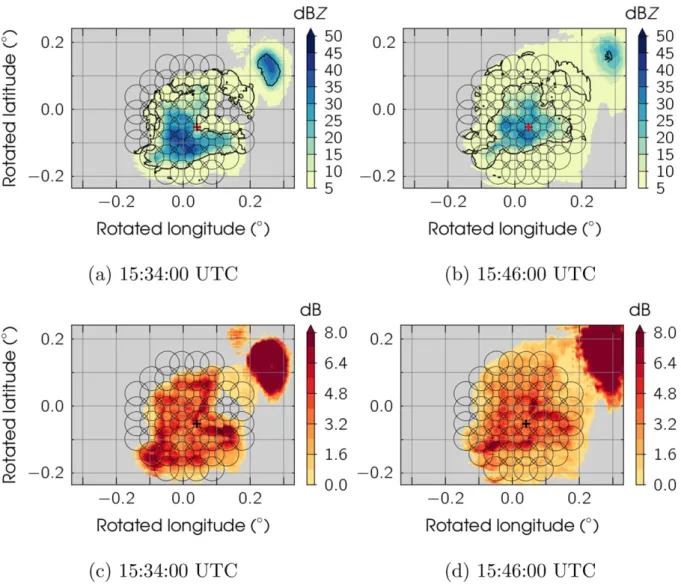
uncertainty is described by the ensemble spread at ana-lysis time, which is shown together with the ensemble mean as an example for two time steps in Fig. 8. The potential of this uncertainty estimate is demonstrated in the following. The new uncertainty estimate is shown to be more accurate than a constant benchmark value, which assumes a constant uncertainty to be representative for the precipitation system. Prior to that, a short verifi-cation of first-order statistics is performed based on pre-cipitation case 1.

Verification is performed at locations selected on a 5000 m5000 m grid, similar to the assimilation loca-tions. The verification grid is shifted by 2500 m in each direction with respect to the assimilation grid in order to select independent observation locations for assimilation

and verification (Fig. 5). The verification grid consists of 47 grid points within X-band radar MOD range. Reflectivity forecasts and observations are compared at verification grid points at each of the eight assimilation time steps, after the update step. Thus, the comparison comprises 376 data points in total.

The overall root mean square error (RMSE) of the forecast ensemble mean for case 1 amounts to 4.49 dB and the bias, defined here as the mean error of the ensemble mean compared to the observations, to 1.54 dB. These forecast statistics can be improved slightly using the probabilistic ensemble information and applying a 80% precipitation probability threshold to the forecast data, i.e. setting the ensemble mean for grid points with precipitation probability lower than 80% to the‘no rain’

Fig. 8. Spatial distribution of the reflectivity ensemble mean (with contour highlighting the region in which 80%of the ensemble members show precipitation above 5 dBZ, top row) and spread (bottom row), i.e. ensemble standard deviation, for the analysis at (a, c) 15:34:00 UTC and (b, d) 15:46:00 UTC on the 03 July 2013. Circles indicate observation influence radii, the cross indicate the location of the observation location used as an example inFig. 7.

value of 5 dBZ. Then, RMSE and bias decrease to 4.44 dB and 1.14 dB, respectively, showing a slight improvement over using model ensemble mean without integrating probabilistic information. The bias indicates an overestimation of precipitation by the forecast model. This is an expected feature considering the simple extrapolation scheme used for the study. Cells can be spread over different regions among the ensemble

members. Especially cell maxima then lead to an overesti-mation of the precipitation by the ensemble mean com-pared to colocated observations. The bias is small compared to the random uncertainty reflected by the RMSE and will have little impact on the results of the proceeding data assimilation experiments. The RMSE of 4.44 dB is approximately 1 dB larger than the estimated accuracy of the original radar data of 3.36 dB (Section 3).

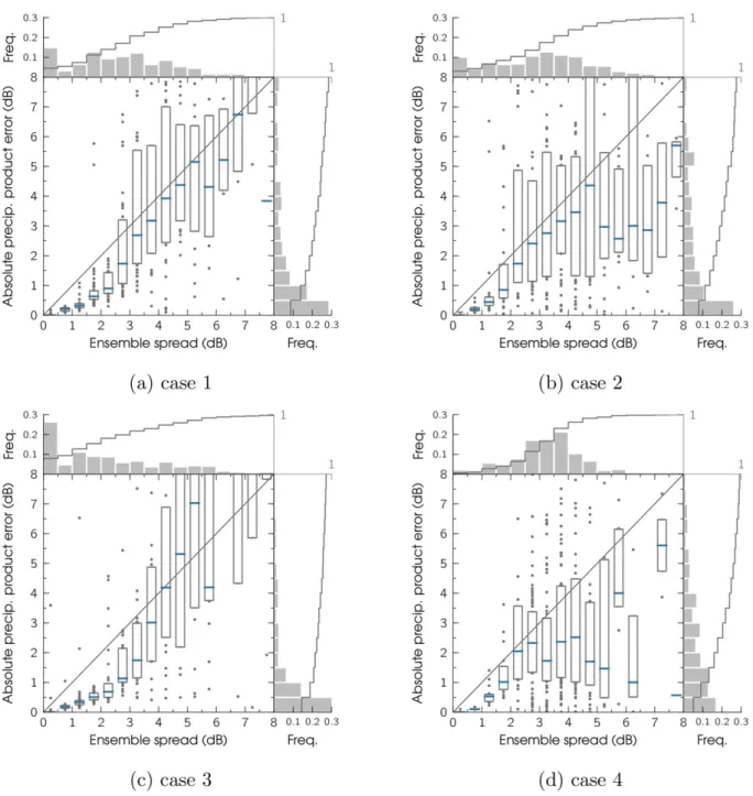
Fig. 9. Comparison of absolute precipitation product (model ensemble mean) error and ensemble spread (model ensemble standard deviation) at the available 47 verification grid points and eight analysis time steps for (a) case 1, (b) case 2, (c) case 3 and (d) case 4. Ensemble spread values are divided into bins of 0.5 dB width, boxes indicate the median (blue line) and the first and third quartiles. Data distribution is shown in frequency histograms, the solid grey lines show the cumulative distribution function.

Considering the simplicity of the nowcasting scheme used here and the forecast range of 30 minutes, results of the forecast ensemble mean are found to be reasonable.

To characterise the quality of the areal uncertainty estimate of the combined precipitation, we analyse the statistical relation between forecasted uncertainty, i.e. the ensemble standard deviation, and the actual error, i.e. the deviation between forecasted and observed reflectivity. In a so-called spread-skill diagram, the perfect relation between forecast uncertainty and forecast error is a one-to-one relation. The uncertainty forecast perfectly describes the uncertainty of the system if, statistically, the actual forecast error equals its forecasted uncertainty (Leutbecher and Palmer, 2008). For all verification grid points, absolute forecast error and corresponding ensem-ble spread are compared in a spread-skill diagram (Fig. 9). Ensemble spread is binned into classes of 0.5 dB width from 0 to 8 dB. Statistics of the absolute forecast error distribution within these classes are described by the median and the first and third quartiles.

Most data points show ensemble spread and absolute product error below 0.5 dB. This category is dominated by grid points without precipitation, both in the forecast and the observations. Overall, there is a clear correlation between ensemble spread and absolute product error, especially for cases 1 and 3, hinting at a good uncertainty representation by the ensemble spread. In the range between 0 and 3 dB ensemble spread, the forecast model ensemble is overdispersive because ensemble spread is substantially larger than the median of the absolute prod-uct error distributions (median below the one-to-one line). This is due to non-zero model forecast values at grid points outside the observed (true) location of the

precipitation cell. Most of the ensemble members cor-rectly predict no precipitation for those grid points, but some have higher reflectivity values because of the differ-ently predicted displacements of the cell. The ensemble standard deviation is more strongly impacted by these few high reflectivity values than the ensemble mean. Therefore, the ensemble standard deviation is larger than the deviation between ensemble mean and observation.

Two scores are defined to quantify the potential of the ensemble spread to correctly represent the uncertainty of the precipitation product in time and space. The aim is to prove that the spatial and temporal structure of the uncertainty estimate is not random, but actually provide valuable additional information. The first score indicates the amount of data points for which the absolute product error falls within the uncertainty range predicted by the ensemble spread—the percentage of ‘hits’. The ensemble spread is interpreted as the tolerated margin of error. The score REL¼100 N XN i¼1 1; ifeiri 0; otherwise (2) represents the reliability of the product uncertainty esti-mate, where ei andriare the absolute forecast error and

the uncertainty estimate for each available verification data point i, respectively. The second score measures the deviation from the perfect spread-skill relation, i.e. from a one-to-one relationship. It is calculated following the definition of the root mean square deviation between ensemble spread and absolute model error at the verifica-tion grid points,

DEV¼ ffiffiffiffiffiffiffiffiffiffiffiffiffiffiffiffiffiffiffiffiffiffiffiffiffiffiffiffiffiffi 1 N XN i¼1 eiri ð Þ2 v u u t _{: (3)}

To assess the areal uncertainty estimate for the com-bined precipitation product, above scores are computed with the spatially and temporally variable product uncer-tainty described by the ensemble spread after the update step at all available verification grid points. The reliability RELvar is computed with ri¼rvar;i; where rvar;i is the product ensemble spread, andei;the corresponding abso-lute difference between forecast ensemble mean and observations from X-band radar MOD at the same grid points and time. For the spread-skill deviationDEVvar;it

is taken into account that the relation between ensemble spread and forecast skill is a statistical one. Therefore, the ensemble spread rvar;i is binned into j classes of 0.5 dB width with class centre rbin;j; as shown in Fig. 9. DEVvar is then computed using rbin;j and the median of the model error distributions in each class, ebin;j: This also reduces the effect of outliers on theDEV score.

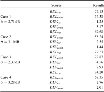
Table 1. Results forREL(%) andDEV(dB) scores for variable uncertainty estimatervarand the constant benchmark valuer:

Scores Results RELvar 77.13 Case 1 RE_Lconst 56.38 r¼2.71 dB DEVvar 1.25 DE_Vconst 3.17 RELvar 69.68 Case 2 RE_Lconst 58.24 r¼3.10dB DEVvar 2.55 DE_Vconst 1.44 RELvar 79.23 Case 3 RE_Lconst 72.87 r¼2.37 dB DEVvar 4.56 DEVconst 7.93 RELvar 74.20 Case 4 RELconst 68.35 r¼3.28 dB DEVvar 2.76 DEVconst 2.01

The benchmark against which the spatially and tem-porally variable uncertainty estimate gained by the flow-dependent ensemble spread is evaluated is a constant uncertainty estimate valid for all grid points at all-time steps. Constant uncertainty information still is most com-mon for precipitation data from radar or other sources (e.g. Tong and Xue,2005; Bick et al.,2016). To facilitate the comparison, the constant uncertainty should conserve the total amount of uncertainty given by the variable uncertainty estimate among the considered data points. In this way, the focus of the analysis is on the ability of the presented method to correctly distribute the available amount of uncertainty information in space and time. Therefore, the chosen reference uncertainty estimate is a mean ensemble spread of the system,r;calculated as an average over the ensemble standard deviation at verifica-tion grid points, including all analysis time steps. In order to compare the spatially and temporally variable uncer-tainty estimate of the combined precipitation product rvar;i to the benchmark, RELconst andDEVconst are

com-puted fromEqs. 2 and3by replacing riby the constant

value forr:

Both scores are summarised in Table 1 for the four precipitation events introduced in Section 4: case 1 with

r¼2.71 dB (convective), case 2 withr¼3.10 dB (strati-form), case 3 with r¼ 2.37 dB (convective) and case 4 with r¼ 3.28 dB (frontal). The reliability REL of the uncertainty forecast improves for all four cases when using the areal uncertainty estimate provided by the data assimilation cycling method compared to using constant benchmark uncertainty estimates. RELvar improves by

36.80 (19.64, 8.73, 8.56) percentage points compared to RELconst for case 1 (case 2, case 3, case 4). This means

that estimate rvar;i provides a more accurate distribution of uncertainty among the system than the reference r: The resulting information on the reliability of the precipi-tation product is therefore improved in all analysed cases, i.e. the tolerated margin of error represented byriis

sat-isfied more often.

The results of theDEV score do not show such a clear signal. DEVvar is reduced by 1.92 dB (3.37 dB), i.e. by

more than a factor of two (one and a half), compared to DEVconst for case 1 (case 3). For case 2 (case 4), theDEV

score does not perform better when usingrbin;jinstead of

r:This is due to areas where the ensemble is overdisper-sive, i.e. where large uncertainty is predicted (ensemble spread) but the error of the precipitation product is mod-erate (exemplarily in the right half ofFig. 9b for case 2). These values occur in a minority of cases but have a large impact on the DEV score after the binning. The large spread among the ensemble members in those few cases may be due to the fact that both events presented in cases 2 and 4 cover a large part of the considered area and

have moderate spatial gradients in the measured precipi-tation fields, which complicates the derivation of displace-ment vectors for the nowcast. An improvedisplace-ment of the results is therefore expected by using a more physically-based probabilistic nowcasting scheme that yields more adequate ensemble members.

6. Summary and conclusions

This article presents a method to estimate spatially and temporally variable uncertainty for a combined areal pre-cipitation product. The method makes use of data assimi-lation to merge precipitation measurements from different sources and an ensemble nowcasting method to evolve the uncertainty estimate over time. The potential of the areal uncertainty estimate provided by the method is demonstrated in a proof of concept study.

Requirements for this improved uncertainty estimate are an accurate representation of the actual error of the initial product, an adjustment to additional observations merged into the product through data assimilation, and flow dependency. In this study, a research network of four X-band weather radar provides reflectivity data for four precipitation cases. Reflectivity can be converted to rain rate using empirical relations that are not part of the analysis.

An ensemble data assimilation method, the LETKF, is used to statistically merge precipitation observations and is coupled to an extrapolation-based nowcasting scheme. The implemented nowcasting scheme computes the cross-correlation between subsequent radar composite images and extrapolates the evolution of the precipitation field using the deduced displacement. The nowcast is started from composite data of the research radar network and a probabilistic forecast is generated using an ensemble tech-nique. The ensemble is generated by stochastic perturb-ation of the computed precipitperturb-ation displacement vectors.

Four data assimilation experiments are performed to test the presented method with emphasis on its potential to provide an improved spatial and temporal uncertainty estimation. We use an ensemble precipitation nowcast and continuously merge observations into the forecast using the LETKF, generating a combined precipitation product. The uncertainty of the precipitation product is estimated by the ensemble spread of the nowcast after each update step of the data assimilation cycle. Two scores are introduced for the assessment of the method. Both are based on the definition of a perfect uncertainty estimate, for which the actual observed error statistically corresponds to the predicted uncertainty. The first score describes the reliability,REL;of the uncertainty estimate. It indicates the percentage of cases in which the actual error of the precipitation product lies within the

estimated uncertainty range. The second score measures the deviation of the uncertainty estimate from a perfect spread-skill relation, DEV; as a root mean square devi-ation between actual error and uncertainty estimate.

The scores are computed at verification grid points selected on a regular grid and for all available analysis time steps. The potential of the obtained areal uncertainty estimatervar;i is assessed by comparison to a benchmark which must be outperformed. The benchmark for this study is defined as the mean spread of the system. In this way, the ability of the method to correctly distribute the available mean uncertainty of the system over time and space can be studied.

The reliability of the uncertainty forecast, REL; is improved by the presented method. The number of hits, i.e. how often the error of the precipitation product is within the tolerated margin of error dictated by the pre-dicted uncertainty range, is increases in all analysed cases. The spread-skill deviation,DEV;is improved in two out of four cases. This score yields unsatisfying results when the spread of the forecast ensemble is large compared to the error of the obtained precipitation product. The large ensemble spread is most likely caused by difficulties in predicting a good sample of displacement fields and large gradients in the precipitation at the edges of the cells in some cases. We expect the results to improve for those cases with a more elaborated probabilistic nowcasting scheme. Despite mixed results for the DEV score, the clear improvement of the uncertainty forecast visible throughout the analysed precipitation events already show that the presented areal uncertainty estimate allows for a more accurate spatial and temporal distribution of the uncertainty information. Since we assume a large impact of the nowcasting scheme on the results for the DEV score, we therefore see potential for further improvement by implementing a more sophisti-cated scheme.

The evaluation of both considered scores demonstrates that the provided areal uncertainty estimate outperforms constant benchmark uncertainty values, but that the method is sensitive to the quality of the probabilistic nowcasting. In subsequent work, the next logical step would therefore be the use of a more sophisticated now-casting tool. Nevertheless, the proof of concept shows the potential of the developed method and establishes the groundwork for further studies. The possible applications of the method are numerous in hydrology, nowcasting or data assimilation. It provides the combination of areal and point measurements for comprehensive precipitation products and additionally yields probabilistic information allowing for the estimation of the product reliability and ensemble generation.

Acknowledgements

Gernot Geppert was supported by the Natural Environment Research Council (Agreement PR140015 between NERC and the National Centre for Earth Observation). We would also like to acknowledge the contributions of the reviewers which led to a significant improvement of the manuscript.

Disclosure statement

No potential conflict of interest was reported by the authors.

References

Alpert, J. C. and Kumar, V. K. 2007. Radial wind super-obs from the WSR-88D radars in the NCEP operational assimilation system.Mon. Weather Rev.135, 1090–1109. doi: 10.1175/MWR3324.1

Atencia, A. and Zawadzki, I. 2014. A comparison of two techniques for generating nowcasting ensembles. Part I: Lagrangian ensemble technique. Mon. Weather Rev. 142, 4036_–4052. doi:10.1175/MWR-D-13-00117.1

Atencia, A. and Zawadzki, I. 2015. A comparison of two techniques for generating nowcasting ensembles. Part II: analogs selection and comparison of techniques.Mon. Weather Rev.143, 2890–2908. doi:10.1175/MWR-D-14-00342.1

Berenguer, M. and Zawadzki, I. 2008. A study of the error covariance matrix of radar rainfall estimates in stratiform rain.

Weather Forecast.23, 1085–1101. doi:10.1175/2008WAF2222134.1 Berndt, C., Rabiei, E. and Haberlandt, U. 2014. Geostatistical

merging of rain gauge and radar data for high temporal resolutions and various station density scenarios. J. Hydrol.

508, 88_–101. doi:10.1016/j.jhydrol.2013.10.028

Bianchi, B., van Leeuwen, P. J., Hogan, R. J. and Berne, A. 2013. A variational approach to retrieve rain rate by combining information from rain gauges, radars, and microwave links.J. Hydrometeorl.14, 1897–1909. doi:10.1175/ JHM-D-12-094.1

Bick, T., Simmer, C., Tromel, S., Wapler, K., Hendricks€ Franssen, H.-J. and co-authors. 2016. Assimilation of 3D radar reflectivities with an ensemble Kalman filter on the convective scale.Q. J. R. Meteorol. Soc.142, 1490–1504. doi: 10.1002/qj.2751

Bishop, C. H., Etherton, B. J. and Majumdar, S. J.2001. Adaptive sampling with the ensemble transform Kalman filter. Part I: theoretical aspects. Mon. Weather Rev. 129, 420–436. doi: 10.1175/1520-0493(2001)129<0420:ASWTET>2.0.CO;2

Bowler, N. E., Pierce, C. E. and Seed, A. W. 2006. STEPS: a probabilistic precipitation forecasting scheme which merges an extrapolation nowcast with downscaled NWP. Q. J. R. Meteorol. Soc.132, 2127_–2155. doi:10.1256/qj.04.100

Chang, W., Chung, K.-S., Fillion, L. and Baek, S.-J. 2014. Radar data assimilation in the Canadian high-resolution ensemble Kalman filter system: performance and verification

with real summer cases.Mon. Weather Rev. 142, 2118–2138. doi:10.1175/MWR-D-13-00291.1

Chumchean, S., Seed, A. and Sharma, A.2006. Correcting of real-time radar rainfall bias using a Kalman filtering approach. J. Hydrol.317, 123–137. doi:10.1016/j.jhydrol.2005.05.013

Chung, K.-S., Zawadzki, I., Yau, M. K. and Fillion, L.2009. Short-term forecasting of a midlatitude convective storm by the assimilation of single-doppler radar observations. Mon. Weather Rev.137, 4115–4135. doi:10.1175/2009MWR2731.1 Ciach, G. J., Krajewski, W. F. and Villarini, G.2007.

Product-error-driven uncertainty model for probabilistic quantitative precipitation estimation with NEXRAD data. J. Hydrometeorl.8, 1325–1347. doi:10.1175/2007JHM814.1 Creutin, J. D., Delrieu, G. and Lebel, T. 1988. Rain

measurement by raingage-radar combination: a geostatistical approach.J. Atmos. Oceanic Technol.5, 102_–115. doi:10.1175/ 1520-0426(1988)005<0102:RMBRRC>2.0.CO;2

Dai, Q., Han, D., Rico-Ramirez, M. and Srivastava, P. K.2014. Multivariate distributed ensemble generator: a new scheme for ensemble radar precipitation estimation over temperate maritime climate. J. Hydrol. 511, 17_–27. doi:10.1016/ j.jhydrol.2014.01.016

Dai, Q., Rico-Ramirez, M. A., Han, D., Islam, T. and Liguori, S.2015. Probabilistic radar rainfall nowcasts using empirical and theoretical uncertainty models. Hydrol. Process. 29, 66_–79. doi:10.1002/hyp.10133

Dowell, D. C., Wicker, L. J. and Snyder, C. 2011. Ensemble Kalman filter assimilation of radar observations of the 8 May 2003 Oklahoma City Supercell: influences of reflectivity observations on storm-scale analyses.Mon. Weather Rev.139, 272_–294. doi:10.1175/2010MWR3438.1

Fielding, M. D., Chiu, J. C., Hogan, R. J. and Feingold, G. 2014. A novel ensemble method for retrieving properties of warm cloud in 3-D using ground-based scanning radar and zenith radiances.J. Geophys. Res. Atmos. 119, 10912–10930. doi:10.1002/2014JD021742

Germann, U., Berenguer, M., Sempere-Torres, D. and Zappa, M. 2009. REALEnsemble radar precipitation estimation for hydrology in a mountainous region.Q. J. R. Meteorol. Soc.

135, 445–456. doi:10.1002/qj.375

Grum, M., Kraemer, S., Verworn, H.-R. and Redder, A.2005. Combined use of point rain gauges, radar, microwave link and level measurements in urban hydrological modelling.

Atmos. Res.77, 313–321. doi:10.1016/j.atmosres.2004.10.013 Haberlandt, U. 2007. Geostatistical interpolation of hourly

precipitation from rain gauges and radar for a large-scale extreme rainfall event. J. Hydrol.332, 144–157. doi:10.1016/ j.jhydrol.2006.06.028

van Horne, MP.2003. Short-Term Precipitation Nowcasting for Composite Radar Rain Fields. Master_’s Thesis, MIT. Hunt, B. R., Kostelich, E. J. and Szunyogh, I. 2007. Efficient

data assimilation for spatiotemporal chaos: a local ensemble transform Kalman filter. Physica D 230, 112–126. doi: 10.1016/j.physd.2006.11.008

Jacques, D. and Zawadzki, I.2014. The impacts of representing the correlation of errors in radar data assimilation. Part I: experiments with simulated background and observation

estimates. Mon. Weather Rev. 142, 3998–4016. doi:10.1175/ MWR-D-14-00104.1

Jacques, D. and Zawadzki, I.2015. The impacts of representing the correlation of errors in radar data assimilation. Part II: model output as background estimates. Mon. Weather Rev.

143, 2637_–2656. doi:10.1175/MWR-D-14-00243.1

Kalman, R. E. 1960. A new approach to linear filtering and prediction problems. J. Basic Eng. 82, 35–45. doi:10.1115/ 1.3662552

Kalman, R. E. and Bucy, R. S. 1961. New results in linear filtering and prediction theory.J. Basic Eng. 83, 95_–108. doi: 10.1115/1.3658902

Krajewski, W. F.1987. Cokriging radar-rainfall and rain gage data.

J. Geophys. Res.92, 9571–9580. doi:10.1029/JD092iD08p09571 Krajewski, W. F. and Ciach, G. J. Towards Probabilistic

Quantitative Precipitation WSR-88D Algorithms: Data Analysis and Development of Ensemble Generator Model: Phase 4. Technical report, NOAA, 02 2006.

Lengfeld, K., Clemens, M., M€unster, H. and Ament, F. 2014. Performance of high-resolution X-band weather radar networks—the PATTERN example. Atmos. Meas. Tech. 7, 4151–4166. doi:10.5194/amt-7-4151-2014

Leutbecher, M. and Palmer, T. N. 2008. Ensemble forecasting.J. Comput. Phys.227, 3515_–3539. doi:10.1016/j.jcp.2007.02.014 Livings, D. M., Dance, S. L. and Nichols, N. K.2008. Unbiased

ensemble square root filters. Physica D237, 1021_–1028. doi: 10.1016/j.physd.2008.01.005

Mercier, F., Barthes, L. and Mallet, C. 2015. Estimation of finescale rainfall fields using broadcast TV satellite links and a 4DVAR assimilation method. J. Atmos. Oceanic Technol.

32, 1709–1728. doi:10.1175/JTECH-D-14-00125.1

Merker, C. 2017. Estimating the Uncertainty of Areal Precipitation using Data Assimilation. PhD thesis, Universit€at Hamburg.

Ott, E., Hunt, B. R., Szunyogh, I., Zimin, A. V., Kostelich, E. J. and co-authors. 2004. A local ensemble Kalman filter for atmospheric data assimilation. Tellus A 56, 415–428. doi: 10.1111/j.1600-0870.2004.00076.x

Park, T., Lee, T., Ahn, S. and Lee, D.2016. Error influence of radar rainfall estimate on rainfall-runoff simulation.Stoch. Environ. Res. Risk Assess.30, 283–292. doi:10.1007/s00477-015-1090-9

Pulkkinen, S., Koistinen, J., Kuitunen, T. and Harri, A.-M. 2016. Probabilistic radar-gauge merging by multivariate spatiotemporal techniques. J. Hydrol. 542, 662–678. doi: 10.1016/j.jhydrol.2016.09.036

Rico-Ramirez, M. A., Liguori, S. and Schellart, A. N. A.2015. Quantifying radar-rainfall uncertainties in urban drainage flow modelling. J. Hydrol. 528, 17–28. doi:10.1016/ j.jhydrol.2015.05.057

Sideris, I. V., Gabella, M., Erdin, R. and Germann, U. 2014. Real-time radarrain-gauge merging using spatio-temporal co-kriging with external drift in the alpine terrain of Switzerland.

Q. J. R. Meteorol. Soc.140, 1097–1111. doi:10.1002/qj.2188 Simonin, D., Ballard, S. P. and Li, Z. 2014. Doppler radar

radial wind assimilation using an hourly cycling 3D-Var with a 1.5 km resolution version of the Met Office Unified Model

for nowcasting.Q. J. R. Meteorol. Soc.140, 2298–2314. doi: 10.1002/qj.2298

Smith, J. A. and Krajewski, W. F.1991. Estimation of the mean field bias of radar rainfall estimates.J. Appl. Meteorol. 30, 397–412. doi:10.1175/1520-0450(1991)030<0397:EOTMFB>2.0.CO;2 Talagrand, O.1997. Assimilation of observations, an introduction.J.

Meteorol. Soc. Jpn75, 191–209. doi:10.2151/jmsj1965.75.1B_191 Tong, M. and Xue, M. 2005. Ensemble Kalman filter

assimilation of Doppler Radar data with a compressible nonhydrostatic model: OSS experiments.Mon. Weather Rev.

133, 1789–1807. doi:10.1175/MWR2898.1

Villarini, G. and Krajewski, W. F. 2009. Empirically based modelling of radar-rainfall uncertainties for a C-band radar at different time-scales. Q. J. R. Meteorol. Soc. 135, 1424–1438. doi:10.1002/qj.454

Villarini, G. and Krajewski, W. F.2010. Review of the different sources of uncertainty in single polarization radar-based estimates of rainfall.Surv. Geophys.31, 107–129. doi:10.1007/ s10712-009-9079-x

Waller, J. A., Dance, S. L. and Nichols, N. K. 2017. On diagnosing observation error statistics with local ensemble data assimilation. Q. J. R. Meteorol. Soc. 143, 2677–2686. doi:10.1002/qj.3117

Waller, J. A., Simonin, D., Dance, S. L., Nichols, N. K. and Ballard, S. P.2016. Diagnosing observation error correlations for Doppler radar radial winds in the met office UKV model using background and observation-minus-analysis statistics. Mon. Weather Rev. 144, 3533–3551. doi: 10.1175/MWR-D-15-0340.1

Xu, Q., Nai, K. and Wei, L. 2007. An innovation method for estimating radar radial-velocity observation error and background wind error covariances. Q. J. R. Meteorol. Soc.

133, 407–415. doi:10.1002/qj.21

Zinevich, A., Messer, H. and Alpert, P. 2009. Frontal rainfall observation by a commercial microwave communication network. J. Appl. Meteorol. Climatol. 48, 1317–1334. doi: 10.1175/2008JAMC2014.1