UNLV Theses/Dissertations/Professional Papers/Capstones
12-2011
Parallel machines scheduling with applications to
Internet ad-slot placement
Shaista Lubna
University of Nevada, Las Vegas
Follow this and additional works at:http://digitalscholarship.unlv.edu/thesesdissertations Part of theDatabases and Information Systems Commons, and theNumerical Analysis and Scientific Computing Commons
This Thesis is brought to you for free and open access by Digital Scholarship@UNLV. It has been accepted for inclusion in UNLV Theses/ Repository Citation
Lubna, Shaista, "Parallel machines scheduling with applications to Internet ad-slot placement" (2011).UNLV Theses/Dissertations/ Professional Papers/Capstones.Paper 1406.
PARALLEL MACHINES SCHEDULING WITH APPLICATIONS TO INTERNET AD-SLOT PLACEMENT
By
Shaista Lubna
Bachelor of Engineering in Computer Science and Information Technology
JNTU University, India May 2006
A thesis submitted in partial fulfillment of the requirements for the
Master of Science Degree in Computer Science School of Computer Science
Howard R. Hughes College of Engineering The Graduate College
University of Nevada, Las Vegas December 2011
THE GRADUATE COLLEGE
We recommend the thesis prepared under our supervision by
Shaista Lubna
entitled
Parallel Machines Scheduling with Applications to Internet Ad-Slot
Placement
be accepted in partial fulfillment of the requirements for the degree of
Master of Science in Computer Science
School of Computer Science
Wolfgang Bein, Committee Chair Ajoy Datta, Committee Member
Lawrence Larmore, Committee Member
Emma Regentova, Graduate College Representative
Ronald Smith, Ph. D., Vice President for Research and Graduate Studies and Dean of the Graduate College
ABSTRACT
Parallel machines scheduling with applications to Internet ad-slot placement.
by
Shaista Lubna
Dr. Wolfgang Bein, Examination Committee Chair Professor, Department of Computer Science
University of Nevada, Las Vegas
We consider a class of problems of scheduling independent jobs on identical, uniform and unrelated parallel machines with an objective of achieving an optimal schedule. The primary focus is on the minimization of the maximum completion time of the jobs, commonly referred to as Makespan (Cmax ). We survey and present examples of uniform machines and its applications to the single slot and multiple slots based on bids and budgets.
The Internet is an important advertising medium attracting large number of advertisers and users. When a user searches for a query, a search engine returns a set of results with the advertisements either on top of the page or on the right hand side. The assignment of these ads to positions is determined by an auction using the ad-slot placement. The algorithmic approach using the level algorithm (which constructs optimal preemptive schedules on uniform parallel machines) is taken into consideration for assigning bidders to the slots on the Internet.
ACKNOWLEDGEMENTS
I would like to thank Dr. Wolfgang Bein for chairing my committee and advising this work. I am thankful for his continuous guidance and help to deepen my work. Without his generous help this thesis would not have had such a rich content. I am thankful to Dr. Ajoy K Datta for his moral support and guidance through my Masters program and help on my thesis. I would also like to specifically thank Dr. Lawrence Larmore and Dr. Emma Regentova for serving on the committee. For this and for being generous with their time when I needed it, I am deeply indebted to them. I would like to thank the faculty at the School of Computer Science, University of Nevada, Las Vegas for the formal education along with generous financial support.
I would also like to extend my appreciation towards my family for being there for me through thick and thin and always encouraging me to strive for the best. Without their endless support I would never be able to reach to the place I’m standing today in my life. Last but not the least; I thank my friends, for their support in the successful completion of this work.
TABLE OF CONTENTS
ABSTRACT...iii
ACKNOWLEDGEMENTS...iv
LIST OF FIGURES...vi
CHAPTER 1 INTRODUCTION...1
CHAPTER 2 PARALLEL MACHINES...6
2.1 Identical Parallel Machines...7
2.1.1 P | pmtn | Cmax ...8
2.1.2 P | pmtn |ri Lmax ...9
2.2 Unrelated Parallel Machines...14
2.2.1 R || Σci ...14
2.2.2 R | pmtn | Cmax, R | pmtn| Lmax and R | pmtn; ri | Lmax ...15
2.3 Uniform Parallel Machines...18
2.3.1 Q | pmtn | Cmax ...18
CHAPTER 3 Application of Level Algorithm...23
CHAPTER 4 Slot Scheduling Theory...39
4.1 Ad slot scheduling...39
4.2 Single-slot...43
4.2.1 Single-slot with budgets- only...43
4.2.2 Single-slot with bids and budgets...45
4.3 Multiple-Slot...48
4.3.1 Multiple-Slot with budgets-only...50
4.3.2 Multiple-Slot with bids and budgets...53
CHAPTER 5 CONCLUSION AND FUTURE WORK...56
BIBLIOGRAPHY...58
LIST OF FIGURES
Figure 1 Machine and Job oriented Gantt charts...2
Figure 2 Optimal schedule for an instance of P | pmtn | Cmax ...7
Figure 3 A network for problem P | pmtn | ri Lmax...11
Figure 4 Example of network for problem P | pmtn | ri Lmax...13
Figure 5 Schedule for problem P| pmtn | ri Lmax...13
Figure 6 Application of the level algorithm...21
Figure 7 Processing 6 jobs jointly on 3 machines...22
Figure 8 Plotting the graph with processing time and speeds....25
Figure 9 Intersection of job 4 and job 5...26
Figure 10 Intersection of job 3, job 4 and job 5...26
Figure 11 Intersection of job 1 and job 2...27
Figure 12 Intersection of all jobs...27
Figure 13 Completion time of all jobs...28
Figure 14 Optimal schedule for 5 jobs...28
Figure 15 Plotting the graph with processing time and speeds....31
Figure 16 Intersection of job 1 and job 2...31
Figure 17 Intersection of job 4 and job 5...32
Figure 18 Intersection of job 3, job 4 and job 5...33
Figure 19 Intersection of all jobs...33
Figure 20 Completion time of all jobs...34
Figure 21 Optimal schedule for 5 jobs...34
Figure 22 Harmonic series diverges …...38
Figure 23 Screen shot of user query with the search results on the left hand the ads on the right...40
Figure 24 Single-slot D clicks...44
Figure 25 Allocation of D clicks...45
Figure 26 Single-slot with budgets and bidders 1,2 and 3...48
Figure 27 Multiple-Slots...51
Figure 28 Allocation of multiple slots with budgets...52
CHAPTER 1 INTRODUCTION
In most manufacturing systems, a decision-making process that plays a crucial role consists in allocating the time at which a particular task is to be processed by a given resource in order to optimize the requirements set by the customer. This function is referred to as scheduling. Indeed, the current economic and commercial market pressures (the growing consumer demand for variety, reduced product life cycle, changing markets with global competition, rapid development of new processes and technologies, etc...) emphasize the need for a system which requires only small inventory levels, minimizes waste production but is able to maintain customer satisfaction by delivering the required goods at the specified time. This requires efficient, effective and accurate scheduling, which is a complex operation in almost all production environments. The importance of scheduling is exemplified by an investigation carried out in the United States mechanical industrial sector which shows that the machines spend about 80% of their total processing time in waiting for the tasks.
Scheduling theory is generally concerned with the optimal allocation of scarce resources to activities over time. More formally, scheduling problems involve jobs that must be scheduled on machines subject to
certain constraints to optimize some objective function. A schedule is for each job an allocation of one or more time intervals to one or more machines [2]. Schedules may be represented by Gantt charts as shown in Figure 1.
A Gantt chart is a type of bar chart that illustrates a project schedule and may be machine oriented or job oriented [2]. (a) and (b) denote the Machine and job oriented Gantt charts respectively.
Graham et al. (1979) introduced the standard α | β | γ notation for representing scheduling problems. This notation embodies the three main elements which define the scheduling problem: the machine environment, the job characteristics, and the optimization criterion. In
the sequel, we briefly detail these three fields. In the considered scheduling models, the number of machines and the number of jobs are assumed to be finite and fixed.
There are several machine environments (represented by the field α) which are summarized in the following:
• Single machine ( α = 1): The process of assigning various jobs to one machine.
• Parallel machines (α = P or Q or R): Each job requires a single operation to be performed on one out of a set of available machines. • Flow shop (α = F ): There are several machines in series. Each job has to be processed on each one of the machines. All jobs have the same routing.
• Job shop (α = J): This model is similar to the flow shop, with the only difference that each job has its own route to follow.
• Open shop (α = O): Likewise the job shop, each job has to be processed on each one of the machines. However, there is no restriction on the routing of each job. The scheduler is allowed to determine the route of any job [1].
Several possible job characteristics (represented by the field β) may modify the scheduling environment. Some of these characteristics are:
• Preemption (pmtn): The processing of any operation may be interrupted and resumed at a later time.
• Precedence constraints (prec): A precedence relation between jobs requires that one or more jobs have to be completed before another job is allowed to start its processing.
• Release dates or heads (rj ): No job can start its processing before its release date.
• Delivery times or tails (qj ): After finishing its processing, each job has to spend an amount of time before exiting the system [1].
The goal of a scheduling algorithm is to produce a ”good” schedule, but the definition of ”good” will vary depending on the application. Therefore, an optimization criterion (represented by the field γ) has to be specified. The most commonly chosen criteria involve the minimization of:
• Makespan (Cmax ): The completion time of the last job to leave the system.
• Maximum lateness (Lmax ): The worst violation of the due dates. The job lateness is non-negative if it is completed late and negative otherwise.
• Maximum tardiness (Tmax ): The difference between tardiness and lateness is that tardiness equals zero if the job is completed early (i.e. Tmax = max(0, Lmax )).
• Maximum flow time (Fmax ): The flow time of a job denotes the time elapsed between its entry to its exit from the system.
• Total (weighted) completion time ( Cj or wjCj ):The sum of the
(weighted) completion times. It indicates the total holding (or inventory) costs incurred by the schedule. This criterion is equivalent to the total (weighted) flow time criterion.
• Total (weighted) tardiness ( Tj or wjTj ): It is a more general cost function than the total (weighted) completion time .
• (Weighted) Number of tardy jobs ( U j or wjUj ): A job is considered as tardy if it is completed after its due date [1].
Thesis Overview: In chapter 2 we survey the types of Parallel machines and approximation algorithms. The applications of the level algorithm is presented in detail in Chapter 3, with suggestive examples. Ad-slot mechanism is reviewed in Chapter 4 with single slot and multiple slots and its illustration. We finish with concluding remarks in Chapter 5.
CHAPTER 2 PARALLEL MACHINES
Given a set of n jobs Jii=1,.. . , n to be processed on m parallel machines M j j=1,. . . , m . Each job Ji has a processing requirement Pii=1,.. . , n and every machine has a speed Sjj=1,. . . , m . Each job requires a single operation to be performed on one out of a set of available machines. The goal is to attain an optimal schedule that specifies when and on which machine each job is to be executed.
The following examples illustrate the role of parallel machines in two different real-life situations.
Example 2.1: Consider the central processing unit of a computer that must process a sequence of programs (jobs) that arrive over time. In what ordering should the programs be processed in order to minimize the average completion time?
Example 2.2: Consider a factory that produces paper bags for cement, charcoal, dog food, and so on. The basic raw material for such an operation is rolls of papers. The production process consists of three stages: printing the logo, gluing the side of the bag, and sewing up one end or both ends. The different bags require different amounts of processing times on different machines. The factory has orders for batches of bags; each order has a date by which it must be completed.
In what ordering should the machines work on different bags in order to ensure that the factory completes as many orders as possible on time?
Parallel Machines can be divided into three classes:
•Identical parallel machines (α = P): All the available machines have the same speed.
•Uniform parallel machines (α = Q): The machines have different
speeds, but these speeds are independent of the jobs.
•Unrelated parallel machines (α = R): The machines have different
speeds, but these speeds are dependent of the jobs [1].
2.1 Identical Parallel Machines :
We consider the problem of scheduling independent jobs on identical parallel machines. Formally there are n jobs Jii=1,.. . , n with processing times pii=1,... , n to be processed on m identical parallel machines M1, . . . , Mm [2].
Mc Naughtons wrap around rule : Compute D=max{max pi,1/mpi} . Assign the jobs in any order from time 0 until time D on machine. If a jobs processing extends beyond time D, preempt the job at time D, and continue its processing on next machine, starting at time 0. Repeat this process until all jobs are assigned [7][18].
2.1.1 P | pmtn | Cmax
Theorem 1: Mc Naughtons wrap around rule is optimal for P | pmtn | Cmax [7].
Proof: It is clear that D is a lower bound for the optimal schedule length. If we can show that wrap around rule can always generate a feasible schedule in the time interval [0,D],then the schedule must be optimal.
i) D≥max{Pi} no jobs can overlap i.e.; simultaneously execute on more than one machine.
ii) mD≥{Pj} as there is enough capacity in the time interval [0,D] to
schedule all jobs.
Thus a wrap around rule can always generate a feasible schedule can be constructed in O(n) time.
2.1.2 P | pmtn; ri | Lmax
Each job Ji has a release time ri and a due date di with ri≤di . To find a preemptive schedule on m identical machines such that the maximum lateness Li is defined as maxni=1{Ci−di} is minimized.
Taking in to account the decision version of the problem: Given some threshold value L there exist a schedule such that
maxin=1L
i=maxi=1
n
{Ci−di}L (1) The above relation holds if and only if
CidiL:=Ld
i for all i=1,. .., n.
All jobs i must finish before the modified due dates diL and cannot
start before the release times ri , i.e. each job Ji must be
processed in an interval [ri, diL] associated with Ji . These intervals are called time windows [2]. We approach the general problem of finding a preemptive schedule for jobs Jii=1,..., n on m identical machines such that all jobs Ji are processed within their interval or time windows [ri, di] by reducing to a maximum flow problem in a network constructed as follows.
Let
t1t2...tr
be the ordered sequence of all different ri values and di values. Consider the intervals
IK:=[tK, tK1]of length TK=tK1−tK for K=1,..., r−1.
We associate a job vertex with each job Ji and an interval vertex with each interval. In addition to the existing nodes we add two dummy vertices source node 's' and target node 't'. Between these vertices, arcs and capacities for these arcs are defined as follows. From s we have an arc to each job vertex Ji with capacity pi and from each interval vertex IK we have an arc to t with capacity mTK .
There exists an arc from Ji to IK if job Ji can be processed in
IK , i.e. iff ritK and tK1di . The capacity of this arc is TK . It is not difficult to prove that there exists a schedule respecting all time windows if and only if the maximum flow in N has the value i=n 1pi . If this is the case, the flow xi on the arc Ji, IK corresponds with the time period in which job Ji is processed in the time interval IK and we have
K=1
r−1
xiK=pi for i=1,. .., n. (2) in=1xiK≤mTK for K=1,..., r−1. (3)
Therefore each job is completely processed and the total amount of processing time in IK is at the most mTK , which is the capacity of m machines.
Furthermore, xiK≤TK for all ( Ji , IK ) ∈ A. (4)
Then there exists a maximal flow satisfying, a feasible solution for the scheduling problem with time windows is constructed by scheduling partial jobs JiK with processing times xiK0 in the intervals IK on m identical machines.
For each K, this is essentially a P | pmtn | Cmax problem, which has a solution with Cmax≤TK because of (3) and (4).
Because network N has at the most O(n) vertices, the maximum flow problem can be solved in O(n3) time. Furthermore, the schedule
respecting the windows can be constructed in O(n2) time. Thus, the window problem can be solved in O(n3) steps [2].
Example: Consider the problem P | ri | Lmax on three machines. Given are processing times p1 = 2, p2 = 2, p3 = 3, p4 = 2. r1 = 0, r2 = 1, r3 =4, r4 = 1. d1 = 5, d2 = 8, d3 = 6, d4 = 8. and let the threshold value L be 3. Use the network flow method with time windows to see if there exists a feasible schedule for the problem L=3. If yes, Draw the schedule.
Solution:
(i) Modify the due dates by dL = L + di . We have d1 = 5 + 3 = 8.
d2 = 8 + 3 = 11. d3 = 6 + 3 = 9. d4 = 8 + 3 = 11.
(ii) Unions of Release times and due dates are 0, 1, 4, 8, 9, 11. The time windows derived are [0,1] [1,4] [4,8] [8,9] [9,11].
IK := [tK , tK+1 ] of length TK = tK+1 − tK for K = 1, . . . r. There exists an arc between Ji and Ik iff job Ji can be processed in Ik i.e; iff ri ≤ Tk and Tk+1 ≤ di. The capacity is Tk.
flow [J1 , I1 ] = 1 flow [J1 , I2 ] = 1 flow [J2 , I2 ] = 2 flow [J3 , I3 ] = 3 flow [J4 , I3 ] = 2 Pi = 2 + 2 + 3 + 2 = 9 The Optimal Schedule is
2.2 Unrelated Parallel Machines
We have n independent jobs i = 1, . . . , n to be processed on m machines. The processing time of job i on machine Mj is pij (i = 1, . . . , n; j = 1, . . . , m). This model is a generalization of the uniform machine model we get by setting pij = pi /sj which is explained in the next section.
2.2.1 R || Ci
R || Ci is reduced to an assignment problem[2]. If i1 , i2 , . . . , ir is the sequence of jobs processed at machine Mj, then the contribution of these jobs in the objective function is
r pi1jr−1pi2j...1pirj
We define a position of a job on a machine by considering the job processed last on the first position, the job processed second from last on the second position, etc. To solve problem R || Ci we have to assign the jobs i to positions k on machines j. The cost of assigning job i to (k, j) is kpij . Note that an optimal solution of this assignment problem has the following property: if some job i is assigned to position k > 1 on machine j, then there is also a job assigned to position k − 1 on machine j. Otherwise, scheduling job i in position k − 1 would improve the total assignment cost (provided that pij > 0). Thus,
solution of the assignment problem always yields an optimal solution of our scheduling problem.
2.2.2 R | pmtn | Cmax , R | pmtn | Lmax and R | pmtn; ri | Lmax
We solve problem R | pmtn | Cmax in two steps. In the first step we formulate a linear program to calculate for each job i and each machine j the amount of time tij machine j works on job i in an optimal schedule. In a second step, a corresponding schedule is constructed. First we give the linear programming formulation. Problem R | pmtn | Cmax is given by nm positive integers pij , which represents the total processing time of job i on machine Mj. Let tij be the processing time of that part of job i which is processed on Mj. Then tij /pij is the fraction of time that job i spends on machine j, and the equation
mj=1 tij pij
= 1
must hold in order for job i to be completed (i = 1, . . . , n). This leads to the following formulation of the problem:
minimize Cmax subject to mj=1 tij pij = 1, i = 1...n. (a) mj=1tij≤Cmax i = 1. ..n. (b) in=1tij≤Cmax j = 1...m. (c)
tij ≥ 0 i = 1. ..n ; j = 1. ..m.
The left-hand side of (b) represents the time job i (i = 1, . . . , n) spends on all machines. The left-hand side of (c) represents the total time machine Mj (j = 1, . . . , m) spends processing jobs. Note that for an optimal solution of this linear program we have
Cmax=max{maxin=1 j=1
m t
ij, maxmj=1in=1tij
The problem of finding a corresponding schedule is equivalent to the problem of finding a solution to the preemptive open shop problem with processing times tij (i = 1, . . . , n; j = 1, . . . , m) which has a Cmax value given by (4). We conclude that problem R | pmtn | Cmax is polynomially solvable.
A similar approach may be used to solve R | pmtn | Lmax. We formulate a linear programming problem to minimize Lmax.
Assume that the jobs are numbered in nondecreasing due date order, i.e. d1 ≤ d2 ≤ . . . ≤ dn.
Let tij1 be the total amount of time that machine Mj spends on job i
in time period I1 = [0, d1 + Lmax ]. Furthermore, for k = 2, . . . , n let tijk be the total amount of time that machine M
j spends on job i within the time period Ik = [dk−1 + Lmax , dk + Lmax ]. Then we have to solve minimize Lmax subject to
mj=1 ki=1 ti j k
mj=1 tij1 ≤ d 1Lmax, i=1,...n j=1 m tij k ≤ dk−dk−1, i=1,. ..n ; k=2,. ..n i=1 n tij 1 ≤ d1Lmax, j=1,. ..m i=kn tijk ≤ d k−dk−1, j=1,...m ; k=2,...n tkij ≥0, j = 1,..., m ; i , k = 1,...n.
Given an optimal solution of this linear programming problem, an Lmax optimal schedule can be obtained by constructing for each of the time periods Ik (k = 1, . . . , n) a corresponding schedule using the data given by the matrix Tk = tijk
. We again conclude that problem
R|pmtn | Lmax is polynomially solvable. In a similar way, we may solve problem R | pmtn; ri | Lmax by considering intervals [tk , tk+1 ], k = 1, . . . , r − 1, where
t1 < t2 < . . . < tr
is the ordered sequence of all ri values and di + Lmax values. In this case, we have the variables tijk and L
max where tkij is the processing time of job i on Mj within the interval [tk , tk+1 ] [2].
2.3Uniform Parallel Machines
We now consider n jobs Ji (i = 1, . . . , n) to be processed on m parallel uniform machines Mj (j = 1, . . . , m). The machines have different speeds sj (j = 1, . . . , m) but the speed of each machine is constant and does not depend on the job. Every job Ji has a processing requirement pi (i = 1, . . . , n). Execution of job Ji on machine Mj requires pi / sj time units. If we set sj = 1 for j = 1, . . . , m. we have m parallel identical machines. All problems with parallel identical machines which are NP-hard are also NP-hard if we replace the machines by uniform machines. Therefore, we consider problems with preemptions. We also assume that 1 = s1 ≥ s2 ≥ ... ≥ sm and p1 ≥ p2 ≥ . . . ≥ pn [2].
2.3.1 Q | pmtn | Cmax
Initially we will present a lower bound ω for the objective value of problem Q | pmtn |Cmax. In the latter step, we will give an algorithm which constructs a schedule of length ω (i.e. an optimal schedule). Let Pi = p1 + . . . + pi and Sj = s1 + . . . + sj for i = 1, . . . , n and j = 1, . . . , m. Furthermore, we assume that n ≥ m. If n < m, we only have to consider the n fastest machines. A necessary condition for processing all jobs in the interval [0, T ] is
Pn = p1 + . . . + pn ≤ s1 T + . . . + sm T = Sm T or
Similarly,the condition Pj /Sj ≤ T should also be for j = 1, . . . , m−1 because Pj /Sj is a lower bound on the length of a schedule for the jobs J1 , . . . , Jj.
Thus,
:=max{maxm−j=11P
j/Sj, Pn/Sm} is a lower bound for the Cmax − values.
Now we will construct a schedule which achieves this bound. The corresponding algorithm is called the level algorithm. Given a partial schedule up to time t, the level pi (t) of job i at time t is the portion of pi not processed before t. At time t, the level algorithm calls a procedure assign (t) which assigns jobs to machines. The machines run with this assignment until some time s > t. A new assignment is done at time s, and the process is repeated [2].
Algorithm level
1: t := 0;
2: WHILE there exist jobs with positive level DO BEGIN
3: Assign(t);
4: t1 := min{s > t | a job completes at time s };
5: t2 := min{s > t | there are jobs i, j with pi (t) > pj (t) and pi (s) = pj (s) };
END
7: Construct the schedule.
The procedure assign(t) is given by
Assign (t)
1. J := { i | pi (t) > 0 }; 2. M := { M1 , . . . , Mm };
3. WHILE J≠ and M≠ DO
BEGIN
4. Find the set I ⊆ J of jobs with highest level;
5. r := min {| M |, | I |};
6. Assign jobs in I to be processed jointly on the r fastest
machines in M;
7. J :=J∖I
8. Eliminate the r fastest machines in M from M
END
The example with 5 jobs to be processed on 4 machines presented below in the figure shows how the algorithm works.
Initially, the four jobs 1,2,3,4 with the largest processing times are processed on machines M1 , M2 , M3 , M4 , respectively. At time t1 job 4 has a level which is equal to the processing time of job 5. Thus, from time t1 jobs 4 and 5 are processed jointly on machine M4. Due to the fact that job 1 is processed on a faster machine than job 2 at time t2 , we reach the situation that p1 (t2 ) = p2 (t2 ). Therefore, jobs 1 and 2 are processed jointly on both M1 and M2 .
To process r jobs 1, . . . , r jointly on l machines M1 , . . . , Ml (r ≥ l) during some time period T, we process each job during a period of T /r time units on each of the machines. A corresponding schedule is shown in the above figure ( 6 jobs 3 machines) for the case r = 6 and l = 3 [2].
CHAPTER 3
Application of the Level Algorithm
EXAMPLE 1: Consider the problem Q | pmtn |Cmax with 5 jobs and 4 machines. Given are the processing times and speeds
P1=5 ; P2=4 ; P3=3 ; P4=2 ; P5=1 .
Harmonic progression is a progression formed by taking the reciprocals of an arithmetic progression. In other words, it is a sequence of the form
a , 1a d ,
a
12d ,
a
13d where -1/d is not a natural number.
(Note: Speeds are in a harmonic progression a=1 and d=1) .
S1=1 ; S2= 1 2 ; S3= 1 3 ; S4= 1 4 .
Construct the optimal schedule using level algorithm and find the value of Cmax ?
Solution: Initially we will present a lower bound for the objective
value of problem Q | pmtn |Cmax.
Let ' n ' be the number of jobs and ' m' be the number of machines. If n < m, we only have to consider the n fastest machines.
A necessary condition for processing all jobs in the interval [0,T] is
Similarly we must have Pj/SjT for j=1,...,m-1 because Pj/Sj is a
lower bound on the length of a schedule for the jobs . Thus J1, . . . , Jj.
:=max{maxmj=−11P
j/Sj, Pn/Sm}
is a lower bound for the Cmax values.
Pn/Sm=54321/10.500.330.25⇒15/2.08⇒7.2115
Similarly for Pj/Sj for j=1,...,m-1. Here m=4 so j = 1, 2, 3
=max{max{5/1,[54/10.5],[543/10.500.33]},7.2115};
=max{max{5, 6, 6.55},7.2115}
=7.2115
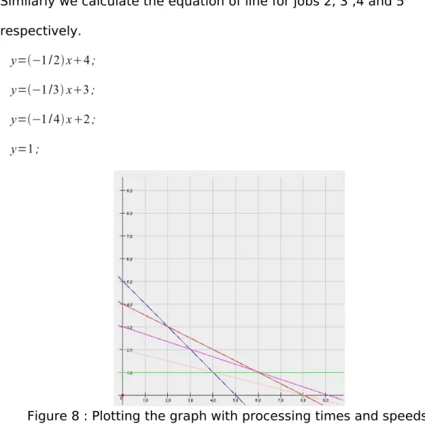
We now plot the graph considering the jobs and speeds on Y- axis and X- axis respectively which results in the t values.
The slope of a line for a job i is considered to be the speed Si . The straight line equation for slope intercept form:
b is the y-intercept and m is the slope.
To find the equation of line that passes through the point (5,0) with a slope of 1 for job J1 is y=−x5
Similarly we calculate the equation of line for jobs 2, 3 ,4 and 5 respectively.
y=−1/2x4; y=−1/3x3; y=−1/4x2; y=1;
Figure 8 : Plotting the graph with processing times and speeds. The first point of intersection is between job 1 and job 2 at (2 , 3) we get t1=2.0 . At this point of time job 1 and 2 are done jointly on machine 1and machine 2.
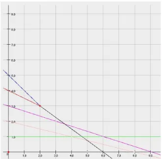
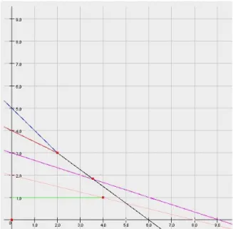
Figure 9 : Intersection of job 4 and job 5.
Similarly at t2 job1, job 2 and job 3 intersect at (3.571, 1.821) the value of t2=3.571
At t2 job 1 , job 2 and job 3 are done jointly on machine 1 ,2 and 3. We now re-plot the graph with the jointly performed jobs J1, J2, J3 .
t3 is the point of time where job 4 and job 5 are done jointly on machine 4 the point of intersection of job 4 and job 5 is (4.0 ,1.0). The value of t3=4.0 .
Figure 11: Intersection of job 1 and job 2.
t4 is the point of intersections of job 1 , job 2 and job 3 with job 4 and job 5 i,e ( 5.422, 0.822). Hence the value of t4=5.422
To calculate t5 we re-plot the graph with the t4 as the point of intersection of (1,2,3,4,5) and slope is considered to be the average of speeds of machines 1,2,3 and 4.
The value of t5=7.9
Final Graph is plotted with t1, t2, t3, t4 and t5 .
Figure 13 : Completion time of all jobs. We now draw the optimal schedule for these jobs.
Example with same processing times but with different speeds. Consider the problem Q | pmtn |Cmax with 5 jobs on 4 machines. Given are the processing times and speeds
P1=5 ; P2=4 ; P3=3 ; P4=2 ; P5=1 .
Harmonic progression is a progression formed by taking the reciprocals of an arithmetic progression. In other words, it is a sequence of the form
a , 1a d ,
a
12d ,
a
13d where -1/d is not a natural number.
Note: Speeds are in a harmonic progression with a=1 and d=0.5 S1=1 ; S2= 1 10.5⇒0.666 ; S3= 1 11⇒0.5 ; S4= 1 11.5⇒0.4 .
Construct the optimal schedule using level algorithm and find the value of Cmax .
Solution: Initially we will present a lower bound for the objective value of problem Q | pmtn | Cmax.
Let ' n ' be the number of jobs and ' m ' be the number of machines. If nm , we only have to consider the n fastest machines.
Pn/SmT
Similarly we must have Pj/SjT for j=1,. .., m−1 because Pj/Sj is a lower bound on the length of a schedule for the jobs J1,..., Jj .
Thus
:=max{maxmj=−11Pj/Sj, Pn/Sm}
Pn/Sm=54321/10.660.50.4⇒15/2.56⇒5.859375
Similarly for Pj/Sj for j=1,. ..m−1
Here m=4 so j = 1, 2, 3
=max{max5/1,[54/10.66],[543/10.660.50],5.859375¿; =max{max{5, 5.4216,5.555},5.8593}
=5.8593
We now plot the graph considering the jobs and speeds on Y- axis and X- axis respectively which results in the t values.
The slope of a line for a job i is considered to be the speed Si . The straight line equation for slope intercept form:
y=m xb where b is the y-intercept and m is the slope.
To find the equation of line that passes through the point (5,0) with a slope of 1 for job J1 is
y=−x5
Similarly we calculate the equation of line for jobs 2, 3 ,4 and 5 respectively.
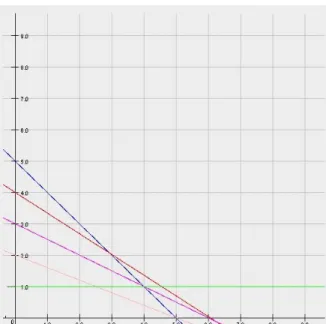
y=−0.666x4; y=−0.5x3; y=−0.4x2; y=1;
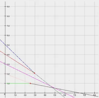
Figure 15: Plotting the graph with processing times and speeds. The first point of intersection is between job 4 and job 5 at (2.5 , 1) we get t1=2.5 . After time t1 job 4 and 5 merge and are processed jointly.
Similarly at t2 job1, job 2 intersect at (2.94, 2.05) the value of
t2=2.94 .
At t2 job 1 and job 2 are done jointly on machine 1 and 2.
We now re-plot the graph with the jointly performed jobs J1 and J2
Figure 17 : Intersection of job 1 and job 2.
t3 is the point of time where job 1,2 and job 3 are done jointly on machine 1, 2 and 3 the time (point)of intersection of all these jobs is (4.5454, 0.7272).The value of t3=4.5454 .
Figure 18 : Intersection of job 1 , job 2 and job 3.
At time t4 job 1,2,3 and 4,5 intersect (4.761 , 0.547) and the value of
t4=4.761
Job 1, 2 and Job 3 are combined with job 4 and 5 and are performed on Machines 1, 2, 3 and 4 and completed at 5.8
Hence the value of t5=5.8 .
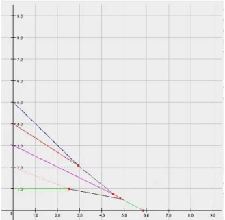
Final Graph is plotted with t1, t2, t3, t4 and t5 .
Figure 20 : Completion time of all jobs. We now draw the optimal schedule for these jobs.
Theorem 2: Algorithm level constructs an optimal schedule for problem Q∣pmtn∣Cmax [2].
Proof :Because
:=max{maxmj=−11P
j/Sj, Pn/Sm}
is a lower bound for the schedule length, it is sufficient to show that the schedule constructed achieves this bound.
Assume that at the beginning of the level algorithm we have p10≥p20≥...≥pn0 . This order does not change during the algorithm, i.e. we have
p10≥p20≥. . .≥pn0 for all t.
We assume that the algorithm always assigns jobs to machines in this order. To prove the desired property, we first assume that no machine is idle before all jobs are finished, say at time T. Then
Ts1...sm=p1p2...pn or T=Pn/Sm
Thus bound is achieved by the algorithm. If a machine is idle before the last job finishes, then for the finishing times f1,..., fm of machines M1,..., Mm we have
Or Else, if fifi1 for some 1≤i≤m−1 , the level of the last job
processed on Mi at some time fi− , where 0 is sufficiently small, is smaller than the level of the last job on Mi1 at the same time. This is a contradiction. Furthermore, in the above equation we have at least one strict inequality.
Assume that T:=f1=f2=...=f jf j1 with jm . The jobs finishing at time T must have been started at time 0. If this is not the case, then we have a job i which starts at time t0 and finishes at time T. This implies that at time 0 at least m jobs, say jobs 1,..., m. are started and processed together on all machines. We have
p10≥...≥pm0≥pi0 , which implies
p1T− ≥...≥pmT−≥piT−0 for all with 0T−t .
Thus, until time T no machine is idle, which is a contradiction. We conclude T=Pj/Sj .
The level algorithm calls the procedure assign(t) at the most O(n) times. The computational effort for assigning jobs to machines after each call is bounded by O(nm). Thus, we get a total complexity of On2m (the total work for calculating all t values is dominated by this).
Theorem 3 : Given a set of parallel machines ‘m ‘ with speeds in harmonic series and jobs ‘n’ with processing times all jobs complete together.
Instead of a formal proof we provide motivation:
We assume that n ≥ m and m = n-1. If n < m, we only have to consider the n fastest machines.
Similarly the speeds of the machines ‘M ‘ are in harmonic series a , 1a
d , a
12d ,
a
13d where -1/d is not a natural number.
To prove that all jobs complete together we use that concept of divergent series.
One way to prove divergence is to compare the harmonic series with another divergent series:
Each term of the harmonic series is greater than or equal to the corresponding term of the second series, and therefore the sum of the harmonic series must be greater than the sum of the second series. However, the sum of the second series is infinite:
It follows that the sum of the harmonic series must be infinite as well. More precisely, the comparison above proves that
for every positive integer k
It can also be proved by the integral test that harmonic series diverges very slowly.
Figure 22 : Harmonic series diverges.
Harmonic series have terms that overlap with the adjacent term there by diverging.
Using the level algorithm and obtaining an optimal schedule with speeds in harmonic progression we observe that the optimal schedule leads to the completion of all jobs at the same time.
CHAPTER 4
Slot Scheduling Theory
As discussed in Chapter 3, the level algorithm produces an optimal schedule. This chapter is divided in two sections. We first discuss the ad-slot scheduling mechanism. In the second part we discuss the application of the level algorithm in Internet ad-slot placement.
4.1Ad-slot scheduling
One of the more visible means by which the Internet has disrupted traditional activity is the manner in which advertising is sold. Offline, the price for advertising is typically set by negotiation or posted price. Online, much advertising is sold via auction. Most prominently, Web search engines like Google and Yahoo! auction space next to search results, a practice known as sponsored search.
Sponsored search is a form of advertising typically sold at auction where merchants bid for positioning along side web search results. Web search engines monetize their service by auctioning off advertising space next to their standard algorithmic search results [27]. For example, Pepsi or sunkist may bid to appear among the advertisements usually located above or to the right of the algorithmic results whenever users search for “soda “.
Figure 23 : Screen shot of user query with the search results on the left and the ads on the right.
These sponsored results are displayed in a format similar to algorithmic results: as a list of items each containing a title, a text description, and a hyperlink to the advertiser’s Web page. We call each position in the list a slot.
Basically, there are three parties involved in sponsored search[22]. • The first party is the advertisers who have multiple objectives in seeking to place advertisements. Some advertisers want to develop their brand, some seek to make sales, and yet others advertise for defensive purposes on specific keywords central to their business. Some have budget constraints, while others are willing to spend as
much as it takes to achieve their goal. Some seek to obtain many clicks and eyeballs, yet others attempt to optimize their return on investment. So, in general, advertisers are of varied types [22].
• The second party is the auctioneer, in this case, the search engine. The search engines have to balance many needs. They must maintain useful search results and have advertisements enhance, rather than interfere with, the search experience. They need to make sure the advertisers get their needs fulfilled, and at the same time ensure that the market the advertisers participate in is efficient and conducive to business.
• The third party is perhaps the most important in the game: these are search users. Users come to search engines for information and pointers. In addition, they also come to discover shopping opportunities, good deals, and new products. There are millions of users with different goals and behavior patterns with respect to
advertisements [22].
Ad slot is a premium ad sales platform used by publishers to increase revenue and significantly reduce cost of sales. The process of choosing and charging the advertisers is a daunting algorithmic and engineering task. The search engines typically take in to consideration several factors including the search key word, the demographics of the user,
the frequency of the keyword, as well as the bid, budget and click through rate of the advertisers for each of these decisions.
We consider the Ad Slot Scheduling problem, where advertisers must be scheduled to sponsored search slots during a given period of time. Advertisers specify a budget constraint, as well as a maximum cost per click, and may not be assigned to more than one slot for a particular search [5].
A natural mechanism for Ad Slot Scheduling is the following: Find a feasible schedule and a set of prices that maximizes revenue, subject to the bidders’ constraints. It is straightforward to derive a linear program for this optimization problem, but unfortunately this is not a truthful mechanism. However, there is a direct truthful mechanism— the price-setting mechanism that results in the same outcome as an equilibrium of the revenue-maximizing mechanism.
Jon et al. [5] derive this mechanism (and prove that it is truthful) by starting with the single-slot case, where two extreme cases have natural, instructive interpretations. With only bids (and unlimited budgets), a winner-take-all mechanism works; with only budgets (and unlimited bids) the clicks are simply divided up in proportion to budgets. Combining these ideas in the right way results in a natural descending-price mechanism, where the price (per click) stops at the point where the bidders who can afford that price have enough budget to purchase all of the clicks.
Generalizing to multiple slots requires understanding the structure of feasible schedules, even in the special budgets-only case. We solve the budgets-only case by characterizing the allowable schedules in terms of the solution (level algorithm) to the problem of Q | pmtn | Cmax. The difficulty that arises is that the lengths of the jobs in the scheduling problem actually depend on the price charged. Thus, we in corporate the scheduling algorithm into a descending-price mechanism, where the price stops at the point where the scheduling constraints are tight; at this point a block of slots is allocated at a fixed uniform price (dividing the clicks equally by budget) and the mechanism iterates.
4.2 Single slot
In this section we consider only one advertising slot with some number of clicks. As mentioned earlier we consider two cases single slot with budgets only and single slot with bids and budgets. We represent the bids as b1,...., bn , budgets as B1,… , Bn and ' D ' as the number of clicks.
4.2.1 Single-slot with budgets-only
Our input in this case is a set of budgets B1,..., Bn , and consider all bids as bi=∞ we are supposed to allocate D clicks with no ceiling on the per-click price. We apply the principle of Proportional sharing
(Proportional Share Scheduling is a type of scheduling which
B
= ∑i Bi. Now to each bidder i, allocate (Bi /B
)D clicks. Set all prices the same: pi = p =B
/D. The mechanism guarantees that each bidder exactly spends his/her budget, thus no bidder will report Bi'Bi . Now suppose some bidder reports Bi'
=Bi− ∆ , for ∆ > 0. Then this bidder is allocated D(Bi − ∆ ) / (
B
− ∆ ) clicks, which is less than D(Bi /B
), since n > 1 and all Bi > 0 [5] [22].Example 1: Suppose there are three bidders and D = 100 clicks in a single slot. Bidder 1 has a budget B1=$25 , bidder 2 has B2 = $15 and bidder 3 has B3= $10. Allocate the number of clicks to each bidder.
Solution: Let us calculate
B
= ∑i BiB
= 25+15+10 = 50.The price for all bidders is p =
B /
D = 50 / 100 => 0.5Allocating the number of clicks for bidder 1 c1 =D *( B1 /
B
) c1 = 100 * ( 25 /50)c1 = 50 clicks.
Similarly, allocating the number of clicks for bidder 2 c2 =D *( B2 /
B
) c2 = 100 * ( 15 /50)c2 = 30 clicks.
Allocating the number of clicks for bidder 3 c3 = D *( B3 / B ) c3 = 100 * ( 10 /50)
c3 = 20 clicks.
4.2.2 Single-slot with bids and budgets.
Let us first assume all budgets Bi = ∞. Then, our input amounts to bids b1 > b2 > . . . >bn. The obvious mechanism is simply to give all the clicks to the highest bidder. We charge bidder 1 her full price p1 = b1. A simple argument shows that reporting the truth is a weakly dominant strategy for this mechanism. The losing bidders cannot gain from decreasing bi. The winning bidder can lower her price by lowering bi, but this will not gain her any more clicks, since she is already getting all D of them. We incorporate the price setting mechanism essentially the descending price mechanism: the price stops descending when the bidders willing to pay at that price have enough budget to purchase all the clicks. We have to be careful at the moment a bidder is added to the pool of the willing bidders; if this new bidder has a large enough budget, then suddenly the willing bidders have more than enough budget to pay for all of the clicks. To compensate, the mechanism
decreases this “threshold” bidder’s effective budget until the clicks are paid for exactly.
Price-Setting (PS) Mechanism (Single Slot with bids and budgets)
• Assume wlog that b1b2. . .bn≥0 .
• Let k be the first bidder such that bk1≤∑ik=1B
i/D . Compute price p=min{∑i=k 1B
i/D , bk} .
• Allocate Bi/p clicks to each i ≤ k −1 . Allocate B
k/p clicks to
bidder k, where B
k=pD− ∑i=1
k −1B
i .
Example 2 : Suppose there are four bidders with b1 = $3, b2 = $2, b3 = $1, b4 = $0.25 and B1 = $20, B2 = $60, B3 = $40, B4 = $5 and D = 100 clicks. Allocate appropriate clicks based on the price-setting mechanism.
Solution: In this case b1b2. . .bn≥0
Case 1: Let k=1 be the first bidder and lets check for the condition bk1≤∑ik=1B i/D b11≤∑i=1 1 Bi/100 b2≤20/100
Let us substitute the value of b2 we get 2≤0.2 This condition does not satisfy.
Case 2 :Let k=2 be the first bidder and lets check for the condition bk1≤∑ik=1B
i/D
b21≤∑i2=1Bi/100 b3≤2060/100
Let us substitute the value of b3 we get 1≤0.8 This condition does not satisfy.
Case 3 :Let k=3 be the first bidder and lets check for the condition bk1≤∑ik=1B i/D b31≤∑i=1 3 Bi/100 b4≤206040/100
Let us substitute the value of b4 we get 0.25≤1.2 This condition satisfies.
Running the PS mechanism we get k = 3 The price is then set as p=min{∑i=1
k Bi/D , bk} p=min{∑i3=1Bi/D , b3} p=min{206040 100 ,1} p=1
Allocating Bi/p clicks to each i≤k−1 we get i≤2as k=3
When i=1 ; 20/1 => 20 clicks are allocated to bidder 1. When i=2 ; 60/1 => 60 clicks are allocated to bidder 2.
Remaining clicks are allocated based on B
k/p clicks to bidder k,
where Bk=pD− ∑ik −=11B
i as per the price setting mechanism.
Bk=pD− ∑ik −=11B
i Here k=3 , p=1, and D=100
Hence B
3=1∗100−2060 we get B3=20
Therefore bidder 1 gets 20 clicks, bidder 2 gets 60 clicks and bidder 3 gets 20 clicks and only $20 of bidder 3 budget is used. There is no threshold bidder.
4.3 Multiple Slots
Generalizing to multiple slots makes the scheduling constraint nontrivial. Now instead of splitting a pool of D clicks arbitrarily, we need to assign clicks that correspond to a feasible schedule of bidders to slots. The conditions under which this is possible add a complexity that needs to be incorporated into the mechanism.
As in the single-slot case it will be instructive to consider first the cases of infinite bids or budgets. Suppose all Bi=∞ . In this case, the input consists of bids only b1b2. . .bn . Naturally, what we do here is rank by bid, and allocate the slots to the bidders in that order. Since each
budget is infinite, we can always set the prices pi equal to the bids
bi . By the same logic as in the single-slot case, this is easily seen to be truthful. In the other case, when bi=∞ , there is a lot more work to do.
Without loss of generality, we may assume the number of slots equals the number of bids (i.e., n′ = n); if this is not the case, then we add dummy bidders with Bi=bi=0 , or dummy slots with Di=0 , as appropriate.
Assigning slots using a classical scheduling algorithm:
First we give an important lemma that characterizes the conditions under which a set of bidders can be allocated to a set of slots, which turns out to be just a restatement of a classical result from scheduling theory.
Lemma 1 [5][22] : Suppose we would like to assign an arbitrary set {1, . . . , k} of bidders to a set of slots {1, . . . , k} with D1. ..Dk . Then, a click allocation c1≥ . .. ≥ ck is feasible iff
c1. . .ck≤ D1. . .Dkfor all l=1,..., k.
Proof: In scheduling theory, we say a job with service requirement x
is a task that needs x/s units of time to complete on a machine with speed s. The question of whether there is a feasible allocation is equivalent to the following scheduling problem: Given k jobs with service requirements xi=ci , and k machines with speeds si=Di ,
there a schedule of jobs to machines (with preemption allowed) that completes in one unit of time ?
As shown in Chapter 3 the optimal schedule for this problem
(a.k.a. Q | pmtn | Cmax ) can be found efficiently by the level algorithm,Level algorithm and the schedule completes in time
maxl ≤ k∑i=l 1x i/∑i=1
l s
i . Thus, the conditions of the lemma are exactly the conditions under which the schedule completes in one unit of time. 4.3.1 Multiple-Slot Budgets-only
This mechanism is roughly a Descending-price mechanism where we decrease the price until a prefix of budgets fits tightly into a prefix of positions at that price, where upon we allocate that prefix, and continue to decrease the price for the remaining bidders. More formally, it can be written as follows [5] [22]:
Price-Setting Mechanism (Multiple Slots, Budgets Only)
• If all Di=0 , assign bidders to slots arbitrarily and exit.
• Sort the bidders by budget and assume wlog that B1≥ B2≥...≥ Bn . • Define rl=∑il=1Bi/∑li=1Di . Set price p=maxlrl .
• Let l∗ be the largest l such that r
l=p . Allocate slots {1,. . . l∗}
to bidders {1,. . . l∗} at price p, using all of their budgets; i.e.,
ci=Bi/p .
• Repeat the steps above on the remaining bidders and slots until all slots are allocated.
Example of Multiple-Slot with Budgets-only :
Suppose there are four bidders A,B,C and D with B1 = $80, B2 = $70, B3 = $20, B4 = $1 and D1 = 100, D2 = 50, D3 = 25, and D4 =0. Allocate appropriate clicks based on the price-setting mechanism for multiple slots with budgets-only.
Solution: In the example Di≠0 so we cannot assign bidders to slot arbitrarily and exit.
We then sort the bidders by budget , but we do not need to sort as they are already sorted in the order B1≥ B2≥...≥ Bn
For l=1 rl=∑il=1Bi/∑il=1Di the value of r1=80/100 Therefore
For l=2 rl=∑i=1 l Bi/∑i=1 l Di the value of r2=[8070/10050] Therefore r2=1
For l=3 rl=∑li=1Bi/∑il=1Di the value of r3=[807020/1005025] Therefore r3=0.971
For l=4 rl=∑il=1Bi/∑il=1Di the value of r4=[8070201/ 1005025] Therefore r4=0.977
Here l∗ =2 since the largest values among r is r2
Allocate slots {1,.. .2} to bidders {1,.. .2} at a price p=1 , using all of their budgets; i.e., ci=Bi/p
c1=B1/p Therefore the no. of clicks c1=80/1 => c1=80
Similarly c2=B2/p Therefore the no. of clicks c2=70/1 => c2=70
We similarly repeat the above steps on the remaining bidders and slots until all slots are allocated.
In the second price block, we get B3/D3=20/25 and
B3B4/D3D4=21/25 . Thus p2 is set to 21/25 = $0.84,
Bidder 3 gets 500/21 (approx 24 ) clicks and bidder 4 gets 25/21 (approximately 1) click, using the schedule as shown.
4.3.2 Multiple-Slots with bids and budgets
The generalization of the multiple slot price setting mechanism to use both bids and budgets combines the ideas from the bids and-budgets version of the single slot mechanism with the budgets-only version of the multiple-slot mechanism. As our price descends, we maintain a set of “active” bidders with bids at or above this price, as in the single-slot mechanism. These active bidders are kept ranked by budget, and when the price reaches the point where a prefix of bidders fits into a prefix of slots (as in the budgets-only mechanism) we allocate them and repeat. As in the single-slot case, we must be careful when a bidder enters the active set and suddenly causes an over-fit; in this case we again reduce the budget of this “threshold” bidder until it fits [5][22].
Price-setting Mechanism ( Multiple slot with Bids and Budgets)
• Assume wlog that b1b2...bn=0.
• Let k be the first bidder such that running price-setting mechanism on bidders 1,...k .would result in a price p≥bk1 .
• Reduce Bk until running price-setting mechanism on bidders
1,..., k would result in a price p≤bk . Apply this allocation, which for some g l∗≤k ives the first l∗ slots to the l∗ bidders among
1,..., k with the largest budgets.
• Repeat the above steps on the remaining bidders and slots until all slots are allocated.
Example for multiple-slots with bids and budgets.
Suppose there are four bidders A,B,C and D with B1 = $80, B2 = $70, B3 = $20, B4 = $1 and D1 = 100, D2 = 50, D3 = 25, and D4 =0 . Bids are also assigned for each bidder b1 = $3 , b2 = $0.75, b3 = $1, b4 = $0.50. Allocate appropriate clicks based on the price-setting mechanism for multiple slots with bids and budgets.
Solution : As per the assumption of w log we are supposed to have
b1b2...bn=0.
We first re arrange the bids which leads to b2 = $1, b3 = $0.75. Running Price-Block mechanism on only bidder 1 gives a price of
r1=80/100 ,
0.8 which is less than the next bid of $1.
So, we re-run Price-Block mechanism on bidders 1 and 3 (the next-highest bid), giving r1=80/100 and r2=100/150 .
We still get a price of $0.80, but now this is more than the next-highest bid of $0.75, so we allocate the first bidder to the first slot at a price of $0.80. We are left with bidders 2-4 and slots 2-4. With just bidder 3 (the highest bidder) and slot 2, we get a price p = 20/50 => 0.4
0.4 which is less than the next-highest bid of $0.75, so we consider bidders 2 and 3 on slots 2 and 3.
This gives a price of max{70/50, 90/75} = $1.40, which is more than $0.50. Since this is also more than $0.75, we must lower B2 until
With this setting of B2 , Price setting allocates bidders 2 and 3 to slots 2 and 3, giving 75(36.25/56.25) and 75(20/56.25) clicks respectively, at a price of $0.75 per click.
Bidder 4 is allocated to slot 4, receiving zero clicks.
Note that by the same logic as the budgets-only mechanism, the prices
CHAPTER 5
CONCLUSION AND FUTURE WORK
In this paper we studied the types of parallel machines in particular we have illustrated examples pertaining to uniform parallel machines and its application in the real world. We have performed various experiments based on the level algorithm and have tried to present the behavior of jobs based on the speeds of machines. When the speeds relating to the machines and processing times were considered to be in a harmonic progression the completion time of all jobs was same.
We have presented a existing mechanism that involves assigning of bidders to the slots based on the classical result from scheduling theory to characterize the possible allocations. The algorithmic approach was taken in to consideration when allocation of ad slots was done based on the level algorithm which is polynomially solvable. As bidders get added in price setting mechanism, maintaining a sorted list of bidders and budgets can be done in time O(n log n). Thus it
remains to show that it can be done in O(n) time given these sorted lists. Computing the ratios rl and allocation can also be done in linear time.
This thesis focuses on technical preview of ad slot scheduling in generating a maximum revenue based on bidders, budgets and slots.
But there could also be many constraints that could improve the quality, efficiency and revenue of the ad slot system which include user click behavior, number and size of slots, advertiser weights.
Bidders can be provided with incentives like payment schemes, refunds and cancellations. An additional aspect of the problem from the auctioneer’s perspective is how to target ads, that is, how to choose the keywords from the surrounding context. Consequently, the the resulting algorithmic approach to revenue maximizing of ad slot scheduling is more intricate and largely unexplored.