Blocked neural networks for knowledge extraction in the software development process

P. Lang, A. Sarishvili, A. Wirsen

Blocked neural networks for

knowledge extraction in the

software development process

© Fraunhofer-Institut für Techno- und Wirtschaftsmathematik ITWM 2003 ISSN 1434-9973

Bericht 56 (2003)

Alle Rechte vorbehalten. Ohne ausdrückliche, schriftliche Gene h mi gung des Herausgebers ist es nicht gestattet, das Buch oder Teile daraus in irgendeiner Form durch Fotokopie, Mikrofi lm oder andere Verfahren zu reproduzieren oder in eine für Maschinen, insbesondere Daten ver ar be tungsanlagen, verwendbare Sprache zu übertragen. Dasselbe gilt für das Recht der öffentlichen Wiedergabe.

Warennamen werden ohne Gewährleistung der freien Verwendbarkeit benutzt.

Die Veröffentlichungen in der Berichtsreihe des Fraunhofer ITWM können bezogen werden über:

Fraunhofer-Institut für Techno- und Wirtschaftsmathematik ITWM Gottlieb-Daimler-Straße, Geb. 49 67663 Kaiserslautern Germany Telefon: +49 (0) 6 31/2 05-32 42 Telefax: +49 (0) 6 31/2 05-41 39

Vorwort

Das Tätigkeitsfeld des Fraunhofer Instituts für Techno- und Wirt schafts ma the ma tik

ITWM um fasst an wen dungs na he Grund la gen for schung, angewandte For schung

so wie Be ra tung und kun den spe zi fi sche Lö sun gen auf allen Gebieten, die für

no- und Wirt schafts ma the ma tik be deut sam sind.

In der Reihe »Berichte des Fraunhofer ITWM« soll die Arbeit des Instituts kon ti

nu ier lich ei ner interessierten Öf fent lich keit in Industrie, Wirtschaft und Wis sen

-schaft vor ge stellt werden. Durch die enge Verzahnung mit dem Fachbereich

the ma tik der Uni ver si tät Kaiserslautern sowie durch zahlreiche Kooperationen mit

in ter na ti o na len Institutionen und Hochschulen in den Bereichen Ausbildung und

For schung ist ein gro ßes Potenzial für Forschungsberichte vorhanden. In die

richt rei he sollen so wohl hervorragende Di plom und Projektarbeiten und Dis ser

-ta ti o nen als auch For schungs be rich te der Institutsmi-tarbeiter und In s ti tuts gäs te zu

ak tu el len Fragen der Techno- und Wirtschaftsmathematik auf ge nom men werden.

Darüberhinaus bietet die Reihe ein Forum für die Berichterstattung über die

rei chen Ko o pe ra ti ons pro jek te des Instituts mit Partnern aus Industrie und

schaft.

Berichterstattung heißt hier Dokumentation darüber, wie aktuelle Er geb nis se aus

mathematischer For schungs- und Entwicklungsarbeit in industrielle An wen dun gen

und Softwareprodukte transferiert wer den, und wie umgekehrt Probleme der

xis neue interessante mathematische Fragestellungen ge ne rie ren.

Prof. Dr. Dieter Prätzel-Wolters

Institutsleiter

Blocked neural networks for knowledge extraction

in the software development process

Patrick Lang, Alex Sarishvili, Andreas Wirsen

October 2003

Abstract

One of the main goals of an organization developing software is to

in-crease the quality of the software while at the same time to dein-crease the

costs and the duration of the development process. To achieve this,

vari-ous decisions effecting this goal before and during the development process

have to be made by the managers. One appropriate tool for decision

sup-port are simulation models of the software life cycle, which also help to

understand the dynamics of the software development process. Building

up a simulation model requires a mathematical description of the

inter-actions between different objects involved in the development process.

Based on experimental data, techniques from the field of knowledge

dis-covery can be used to quantify these interactions and to generate new

process knowledge based on the analysis of the determined relationships.

In this paper blocked neuronal networks and related relevance measures

will be presented as an appropriate tool for quantification and validation

of qualitatively known dependencies in the software development process.

Keywords:

Blocked Neural Networks, Nonlinear Regression,

Knowl-edge Extraction, Code Inspection

1

Introduction

During the last years various simulation tools focusing on different aspects in the

software development process were presented in the literature. They roughly can

be classified into continuous (system dynamics), discrete event or hybrid

simu-lation models. We especially are involved in developing a discrete event model,

which focuses mainly on the inspection process in the coding phase and the

test phase of the software life cycle (see [6],[7]). In comparison to a continuous

simulation model, choosing a discrete event approach allows a more detailed

representation of the organizational issues, products and resources. It is i.e.

possible to model programmers or inspectors with different skills or to consider

different types of software items with varying complexity and size.

Building up a simulation model requires the determination of input output

re-lationships at the different sub-processes of the software development process,

which are in case of considering a waterfall model the requirement, design,

cod-ing and test phase. In software engineercod-ing the software development process is

described by static qualitative models like control diagrams, flow diagrams and

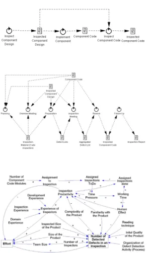
cause-effect diagrams. Figure 1 shows as an example the control diagram, the

flow diagram and cause-effect diagram of an inspection process. These models

are in contrast to a simulation model not appropriate to study the dynamic

ef-fects occurring during the software development process. However, they provide

a general understanding concerning the chronology of tasks (control diagram),

the flow of the objects (flow diagram) and the qualitative dependencies of

ob-jects (cause-effect diagrams) and thus include the basic information needed for

building up a simulation model.

Figure 1: Qualitative models of the software inspection process. Top: Control

Diagram. Middle: Flow Diagram. Bottom: Cause-Effect Diagram

simula-tion model is explained. The model can be built by following step by step the

control and flow diagram (see figure 1). In this way activity blocks inside the

simulation model with their related inputs and outputs, i.e. items, stuff, etc.,

are determined. Inside an activity block the relationships between certain

vari-ables, qualitatively described by the corresponding cause-effect diagrams, then

have to be quantified by mathematical equations or logical rules. A cause-effect

diagram generally distinguishes between three types of variables:

•

process input variables, which do not depend on other variables,

•

process output variables, which do not effect other variables and

•

internal process variables, which are explaining other variables and are

also explained by other variables.

Based on the cause-effect diagram one step by step chooses each of the

internal and output variables as the explained variable and their corresponding

predecessors as explaining variables. The related input output relationships

then have to be determined as a logical rule or a mathematical function.

Possible methods for quantifying the qualitatively known input output

re-lationships are expert interviews, pragmatic models, stochastic analysis and

knowledge discovery techniques. The choice of the actual technique depends

of course on the data or information available, i.e. measurement data from

experiments, linguistic descriptions, etc..

In this paper we assume that sufficient measurement data is given such that

an application of knowledge discovery techniques is possible. In a first step these

methods will be used for the quantification of the input output relationships.

Then, based on the identified mappings, new insight and rules for parts of the

considered process will be generated. In the example at the end we investigate

mathematical descriptions determining the

number of major defects found in an

inspection process

depending on the

effort

, the

size of the products

and other

variables as can be seen in the related cause-effect diagram (see figure 1).

The simplest approach for the quantification of an input output relationship

in form of a mathematical equation is to consider a linear regression problem:

x

=

d

i=1

Y

a

+

, j

= 1

, . . . , n,

where

x

∈

R

contains the j-th measurement of the output variable,

Y

∈

R

are vectors containing the measurements of the related input variables,

a

∈

R

denote the d unknown regression coefficients and

is the measurement error of

the j-th variable.

However, due to saturation effects the influence of some of the input

vari-ables, like

skills of programmers or inspectors

or other human and document

properties, obviously is nonlinear. Therefore it seems quite reasonable to use a

generalized regression model.

More especially, we will consider an additive nonlinear regression model (AN)

of the form

x

=

i

a

m

(

Y

) +

, j

= 1

, . . . , n,

where

m

:

R

→

R

, i

= 1

, . . . , d

are nonlinear twice differentiable functions

depending on further regression coefficients and

a

∈

R

are again regression

co-efficients. AN models are reasonable generalizations of classical linear models,

since they conserve the interpretability property of linear models and

simul-taneously are able to reproduce certain nonlinearities in the data. It also is

possible to calculate and interpret the partial derivatives of an AN model. The

importance of the partial derivatives lies in relevance and sensitivity analysis.

The additive nonlinear regression function can be approximated by different

methods. The most common of them are so called back fitting algorithms [8]

with various smoothing operators, like:

•

Univariate regression smoothers such as local polynomial regression.

•

Linear regression operators yielding polynomial or parametric spline fits.

•

More complex operators such as surface smoothers.

In this paper we consider specially structured (block-wise) neural networks

for the estimation of the AN model. In [4], [9] it was shown that fully

con-nected neural networks are able to approximate arbitrary continuous functions

with arbitrary accuracy, furthermore in [10] it was proven that neural networks

are able to approximate the derivatives of regression functions. This result was

assigned in [16] to block-wise neural networks as estimators for nonlinear

addi-tive twice continuously differentiable regression functions and their derivaaddi-tives.

The network function consists of input and output weights for each unit in the

hidden layer, which have to be estimated from given measurement data. This

is done by minimizing the mean squared error over a training set. The

perfor-mance of the network is measured by the prediction mean squared error, which

is estimated by cross validation [3].

The network function estimated by the neural network will be used when the

model is created, i.e. it will be implemented in the model at the considered node

of the cause-effect diagram to calculate the output for a given input during the

simulation is running. Here one has to mention, that the structure of the

net-work in general remains unchanged for the developed simulation model since it

is based on qualitative models while the weights of the network function might

change for different software development processes and thus the neural network

has to be retrained with respect to the considered process. In the simulation

model the values of input variables of the equations have to be provided in the

considered activity block.

Now it will be shown that relevance measures calculated on the identified

network function also are an important tool in the context of the software

de-velopment process. The problem, which often occurs especially in modelling

the software development process is, that not for all input variables

measure-ment data are available. The granularity of the model determines the minimal

amount of measurement data needed for rule generation since all input and

out-put variables of the underlying qualitative model should be used at this step.

In case of missing measurement data for one or more variables one has to make

further assumptions or skip these variables. Relevance measures in this case

help to determine the impact of each input variable with respect to the output

variable. By considering the validation results and the corresponding relevance

measure, one can easily verify whether the estimated functional dependencies

describe the input output relationship in a sufficient manner, if the impact of

a skipped variable is too large or if an explaining (input) variable is missing

in the underlying qualitative model. In the latter case, the missing variable

should be determined by analyzing the set of all measured variables e.g. by

a case-based-reasoning method (see [20]) and a new rule has to be generated

for by incorporating the identified missing input variables or by applying other

knowledge discovery techniques. If a variable has only small relevance over its

whole measurement range it is redundant, i.e. it does not explain the

consid-ered output and thus can be skipped. Thus, a relevance measure can also be

used to validate the qualitative description of the dependencies given in the

cause-effect diagrams since the inputs for a node in the diagram are assumed

to be not redundant. Also the size of the impact of every input variable for a

given data set is available and might give the manager a new insight into the

considered software development process. Thus, the relevance measure might

help to provide the manager a new rule of thumb.

Using the blocked neural network approach two aspects mentioned above

will be considered, which are

1. the quantification of the qualitative models

2. and analyzing of the determined mathematical equations in order to find

a more deep insight into the input output relationship by relevance or

sensitivity analysis.

Currently, we analyze data on historical software development processes coming

from a large company. Unfortunately, these data (which were not collected for

the purpose of fitting a simulation model) cover only some of the variables

re-quired for building the desired discrete event simulation model of the inspection

process. For instance, considering the cause-effect diagram of the inspection

process (see figure 1), information on the assignment of tasks to persons, skills

and individual working times is missing. However, our approaches from neural

networks describe an appropriate idea how the input output relationship could

be achieved and how to determine the impact of the input variables with respect

to the considered output based on the identified mapping.

2

Neural network modelling

Neural networks provide a convenient language game for nonlinear modelling.

They are typically used in pattern recognition, where a collection of features is

presented to the network, and the task is to assign the input to one or more

classes. In [13] it is shown that arbitrary complex decision regions, including

concave regions, can be formed using four-layer neural networks. In [11] the

abil-ity of three-layer networks to form several complex decision regions in pattern

recognition applications is demonstrated by simulations.

Another typical use for neural networks is the field of nonlinear regression

problems. In [2], [4], [9], [1], it is shown independently, that neural networks

with linear output and single hidden layer with sigmoid activation function can

approximate any continuous regression function uniformly on compact domains.

Neural networks typically exhibit two types of behavior. If no feedback loops

are present in the network connections, the signal produced by an external input

moves in only one direction and the output of the network is given by the output

of the last layer neurons. In this case a neural network behaves mathematically

like a static nonlinear mapping of the inputs. This feedforward type of networks

therefore is most often used for nonlinear function approximation. The second

kind of network behavior is observed when feedback loops are present. In this

case the network behaves like a dynamical system, and the outputs of the

neu-rons are functions of time. The neuron outputs can for example oscillate, or

converge into a steady state.

In this paper we consider feedforward neural networks with one hidden layer

to solve regression problems occurring during modelling the software life cycle.

The structure of such a neural network is depicted in figure 2.

w

v

v

v

φ

φ

φ

Σ

1

1

v

y

y

y

w

w

w

w

w

x

Figure 2: Feedforward neural network.

The output of the feedforward neural network is computed as:

f

(

Y, θ

) =

v

+

H

h=1

v

φ

Y

·

w

,

(1)

where

θ

= (

w

, ..., w

, v

, ..., v

) is the vector of network weights, with

w

=

(

w

, ..., w

) for

h

= 1

, ..., H

and

H

denotes the number of neurons in the

hidden layer. Moreover,

φ

is the activation function from each hidden unit

and

Y

= (1

, y

, ..., y

) denotes the vector of inputs. More about the special

architecture of the neural networks considered in this paper will be discussed in

the next sections.

Based on the given input output data the network parameters are estimated

via convenient learning algorithms. In the case of feed forward networks usually

a variant of the famous backpropagation algorithm is used.

2.1

Variable significance testing

If one not only is interested in obtaining a good input output approximation,

but one further wants to get more insight into the structure of the underlying

function, different postprocessing methods can be applied to the trained

net-work. In order to derive the significance of each neural network input variable

based on the derived function various statistical hypothesis tests can be used.

In general, this involves the following main steps:

•

the definition of a convenient relevance measure,

•

estimating the defined relevance of each input variable with respect to the

corresponding model output,

•

estimating the sampling variability of the selected relevance measure,

•

testing the null hypothesis of irrelevance.

In the next section we introduce some classical relevance measures that are

often used in the case of neural networks.

2.2

Classical relevance measures in the neural network

ap-proach

We consider the following regression problem:

x

=

M

(

y

, ..., y

) +

, i

∈

[1

, ..., N

]

,

where

is i.i.

N

(0

, σ

) distributed noise, the function

M

:

R

_→

_R

_{is Borel}

measurable and twice differentiable at any

i

∈

[1

, ..., N

]. We now approximate

the true regression function

M

with a neural network approximator:

ˆ

x

=

f

(

y

, ..., y

,

θ

ˆ

) +

,

ˆ

θ

=

arg

min

(

x

−

f

(

y

, ..., y

,

Θ))

,

The most common measure of relevance is the average derivative (AD), since

the average change in ˆ

x

for a very small perturbation

δy

−→

0 in the

indepen-dent variables

y

is simply given by:

AD

(

y

) =

1

N

∂

ˆ

x

∂y

,

(2)

where ˆ

x

is the vector of estimated regression outputs. Sometimes ˆ

x

is sensitive

to

y

only for a small percentage of input vectors

y

. Such requirements give

rise to the following measure of relevance, that can be quite important in the

context of particular applications.

M axD

(

y

) =

max

∂

x

ˆ

∂y

.

Another quantification of ˆ

x

’s sensitivity to

y

, is the average percentage change

in ˆ

x

for a one percent change in

y

, a measure that is commonly known as the

”Average Elasticity” of ˆ

x

to

y

[15]:

AvE

(

y

) =

1

N

∂

x

ˆ

∂y

y

ˆ

x

,

x

ˆ

= 0

∀

i

= 1

, ..., N.

(3)

Another measure describes the average contribution of the

y

’s to the

mag-nitude of the gradient vector. Therefore a measure of sensitivity, namely the

”standard deviation” of the derivatives across the sample measuring the

disper-sion of the derivatives around their mean, is computed:

SD

(

y

) =





1

N

_∂y

∂

x

ˆ

−

_N

1

∂

x

ˆ

∂y





.

Normalizing

SD

(

y

) by the mean, provides us with the coefficient of variation

that is the standard deviation per unit of sensitivity:

CV

(

y

) =

SD

(

y

)

.

All the described relevance measures share the disadvantage that for

stan-dard (fully connected) feedforward networks, the partial derivatives in general

depend on all input variables. Therefore the interpretation in terms of the

rele-vance of a single input variable is difficult. One method to avoid this problem is

to set all variables except the considered variable

y

to their mean values. This

however leads to a significant loss of information. Another method consists in

using blocked neural networks as universal function approximators, a method

that is described in the next sections.

At the end of this paper we will compare and discuss the results of a relevance

analysis for a software development process based on the measures

AD

and

AvE

.

2.3

Additive nonlinear(AN) regression models

As described before, we use ANs for understanding software development

pro-cesses profiting from the advantages of ANs, like interpretability and flexibility,

compared to other methods. In this section we define a general form AN model

and state main assumptions that should be fulfilled if ANs are chosen for

mod-elling.

Let

Y

∈

R

_{be a design data matrix, where each column refers to a}

sin-gle observation and each row to an attribute. In the following we describe an

additive nonlinear regression problem.

Assumption 2.1.

The function

M

:

R

_−→

_R

_{that describes the true}

relation-ship between the dependent variables

x

∈

R

, i

= 1

, ..., N

, and the data design

matrix

Y

exists.

Assumption 2.2.

The conditional expectation function

M

:

R

_−→

_R

_,

M

(

Y

) =

E

{

x

|

(

y

, ..., y

) =

Y

}

has an additive structure, i.e.

M

(

Y

) =

m

(

y

) +

...

+

m

(

y

)

,

where

m

:

R

−→

R

,

∀

j

= 1

, ..., d

.

Definition 2.3.

An Additive Nonlinear (AN(d)) model for any variable

x

∈

R

, i

= 1

, ..., N

is defined by,

x

=

m

(

y

) +

...

+

m

(

y

) +

, i

= 1

, ..., N

(4)

where

is i.i.

N

(0

, σ

)

distributed with finite variance.

In the course of this paper we estimate the function

M

by fitting feedforward

neural networks with block structure to the data.

The optimal network hereby is determined by minimizing the mean squared

prediction error.

2.4

AN model estimation with blocked neural networks

Taking into account the special structure of the composite function

M

, which

results from summing up

d

functions of mutually different real variables, a

feed-forward network with one hidden layer and without ”nonparallel” input to

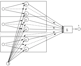
hid-den layer connections seems to be convenient for its approximation. Figure 3

1 2 d φ

Σ

Figure 3: Blocked neural network.

shows such a blocked neural network with

d

inputs and one output. Especially,

each neuron in the hidden layer accepts only one variable as input apart from

the constant bias node.

The output of the blocked neural network is given as:

x

=

f

(

y

, ..., y

,

Θ)

=

v

φ

(

y

w

+

b

) +

...

+

v

φ

(

y

w

+

b

)

,

(5)

where the difference

H

(

j

)

−

H

(

j

−

1)

,

∀

j

= 2

, ..., d

is the number of neurons in

block

i

, and

H

(

d

) denotes the total number of neurons in the hidden layer. The

w

s are the weights from the input to the hidden layer, the

v

s are the weights

from the hidden to the output layer, the

b

s are the biases and Θ denotes

the vector of all neural network parameters together. The neuron activation

function is chosen to be of sigmoidal type, i.e.:

φ

(

x

) =

ex+e−x

.

The neural network training consists of minimizing the mean squared error

over all training samples resulting in the optimal network parameters:

ˆ

θ

=

arg

min

(

x

−

f

(

y

, ..., y

,

Θ))

,

where Θ

is a compact subset of the parameter space. In the following the

supscripts of f are skipped.

The following theorem describes the approximation abilities of such a neural

network.

Theorem 2.4.

Let

φ

(

·

)

be a nonconstant, bounded and monotonic increasing

continuous function. Let

K

be a compact subset of

R

and

k

≥

1

a fixed integer.

Then any continuous mapping

F

:

K

−→

R

with

F

(

y

, ..., y

) =

f

(

y

) +

...

+

f

(

y

)

, where

f

:

R

−→

R

,

j

= 1

, ..., d

are continuous and

K

⊂

Domain

(

f

)

,

can be approximated in the sense of uniform topology on K by blocked networks

with one hidden layer, where the hidden layer functions are chosen as

φ

(

·

)

and

the input and output layer are defined by arbitrary linear functions.

This theorem is identical to the general theorem presented by [4] except the

assumption that the function

F

is a sum of

d

continuous functions and therefore

continuous itself. Thus the proof is analogous to the proof in [4].

Note, that multilayer feedforward neural networks not only are capable of

arbitrary accurate approximations for unknown mappings, but further they also

can be used to estimate simultaneously the related derivatives, see [10].

2.4.1

Derivatives in blocked neural networks.

In this section we derive the important property of blocked neural networks

consisting in the special relation between the expected partial derivatives of the

network function with respect to the input variables and the partial derivatives

with respect to the network weights. For simplification we consider a blocked

neural network with only one neuron in each block, see figure 4. All results

shown in this section are also transferable to arbitrary connected blocked neural

networks.

w

w

w

v

v

v

φ

φ

φ

Σ

1

1

v

y

y

y

w

w

w

x

Figure 4: Blocked neural network with one neuron in each block.

The considered network function then has the form:

f

(

y, θ

) =

v

+

d

j=1

where

y

is the

j

-th coordinate of

y

. If

φ

is differentiable, as we always assume,

the derivatives w.r.t.

y

and w.r.t. the parameter

w

are given as:

∂f

(

y, θ

)

∂y

=

v

φ

₍

_w

+

w

y

)

w

∂f

(

y, θ

)

∂w

=

v

φ

₍

_w

+

w

y

)

y

.

Based on these identities the following theorem can be proven.

Theorem 2.5.

For a blocked neural network with one neuron in each block, we

consider

C

:=

E

∂f

(

y, θ

)

∂w

,

R

:=

E

∂f

(

y, θ

)

∂y

,

R

:=

E

∂f

(

y, θ

)

∂y

.

a) If the

j

-th input variable is bounded with essential supremum

||

y

||

, then

|

w

|

C

≤ ||

y

||

R

b) In general, we have

|

w

|

C

≤

E

(

|

y

|

)

R

.

Proof

a)

C

=

E

∂f

(

y, θ

)

∂w

=

|

v

|

E

|

φ

(

w

+

w

y

)

| · |

y

|

≤ |

v

| · ||

y

||

E

|

φ

(

w

+

w

y

)

|

=

||

y

||

|

w

|

E

∂f

_∂y

(

y, θ

)

=

||

y

||

|

w

|

R

b)

C

=

E

∂f

(

y, θ

)

∂w

=

v

E

|

φ

(

w

+

w

y

)

| · |

y

|

≤

v

E

(

|

φ

(

w

+

w

y

)

|

)

E

(

|

y

|

)

=

E

(

|

y

|

₎

w

E

∂f

(

y, θ

)

∂y

=

E

(

|

y

|

₎

w

R

,

where the inequality is derived using Bunjakowski-Schwarz.

The theorem tells us that

R

and

R

may be interpreted as relevance measures

of the

j

-th input variable with respect to the considered network output. If e.g.,

R

is smaller than either

|

w

|

or the mean of

or if both expressions are

small, then the

j

-th hidden neuron, describing the dependency of the network

output on the variable

y

is negligible.

For the sake of completeness, we state this qualitative property which is also

applied in other parts of neural network theory, as a lemma.

Lemma 2.6.

Under the conditions of Theorem 2.5, the

j

-th variable

y

has

little influence on the network output, if the derivative

j

is small in average

measured by either

R

or

R

.

Remark 1.

In the case of

φ

being the identity, the neural network function

reduces to

f

(

y, θ

) =

v

+

v

w

+

v

w

y

.

In that case,

R

becomes

|

v

·

w

|

. So

R

is the coefficient of the input variable

y

. Obviously, the influence of

y

for the output is small, whenever

R

is small

2.4.2

Relevance measures and partial derivative plots

As already discussed in the previous sections relevance measures estimated from

regression functions can be used to determine the impact of every single input

variable with respect to the considered output.

In the linear case the partial derivatives coincide with the regression

coeffi-cients and thus are constants. In the case of a general nonlinear differentiable

regression model the computation of the relevance measures also is possible,

however in order to guarantee the interpretability of the results further

struc-tural properties have to be fulfilled. For AN models, like the considered blocked

neural networks, these properties hold (see section 2.4) and therefore the

im-pacts of the single input variables can be estimated.

In the following it will be explained, how a relevance measure and the partial

derivative plots are derived and how they are interpreted.

In order to compute the different relevance measures, the first partial

deriva-tives

∂yj

of the trained network function

f

(

·

,

Θ) with respect to each explaining

variable

y

,

j

∈ {

1

, . . . , d

}

have to be determined. For the sigmoid neuron

acti-vation function of the network, the partial derivatives are calculated via:

∂f

(

y

, . . . , y

,

Θ)

∂y

=

H

i=H(j−1)+1

v

1

−

tanh

(

b

+

w

y

)

w

, j

= 1

, . . . , d,

(6)

where

H

(

j

) is defined as in equation (5). Obviously, the partial derivative

explicitly only depends on the considered input itself, the influences of the other

variables is comprised in the network parameters Θ.

The partial derivative (PD) themselves already can be used to analyze the

impact of the input variables. Therefore, for each of the input variables a plot is

generated from the corresponding partial derivative, that is evaluated for each

given data pair. A large PD-value indicates that the influence of the related

input variable is strong for the considered output value, already small changes of

the input value will cause large changes on the output value. Vice versa a small

PD-value is an indicator for a weak dependency. Moreover, if the PD-values for

a certain input variable are small for all input values, then it is not considered

to be an explaining variable, i.e. it is redundant. If for a certain range of the

output all PD-values of all model input variables are small, then there is no

clear causal relationship between the inputs and the output at this range. One

reason for such an observation might be a missing input variable. Furthermore,

a positive PD-value indicates that an increase in the input value will lead to

an increase in the output value, whereas a negative PD-value indicates that an

increase in the input will lead to a decrease in the output. Although each of

the PD-values contains relevant information concerning the impact the related

input variable, due to outliers in the data set those interpretations could be

erroneous. Therefore one always should consider the PD-values of a complete

input interval, where one especially should focus on those ranges with a sufficient

number of data available.

Based on equation (6), the chosen relevance measure is computed by

eval-uating the corresponding equation for the given data set. In the following we

especially focus on the AD and AvE relevance measure.

The AD relevance measure estimates the mean influence of the input variable.

This number however should be interpreted with care, since i.e. a small

AD-value could be the result of the sum of large positive and large negative

PD-values. This measure also describes how changes in the output and the input

values are correlated in the mean. A positive AD-value indicates that in the

mean a positive change of the input value will increase the output value whereas

a negative AD-value indicates that the output value will decrease under such

input changes. The average elasticity (AvE) determines the average percentage

change in the output value assuming a one percent change in each of the input

values.

3

Quantification and analysis of an input

out-put relationship in the software development

process

In this section we apply the presented methods to an inspection process (coding

phase), being a part of the overall software development.

Figure 1 shows the qualitative models related to this process, i.e. the control

diagram, the flow diagram and the cause-effect diagram.

On the way to an implementation of the inspection process in terms of a

discrete event simulation model, one important step is the quantification of the

occurring input output relationships given as nodes in the related cause-effect

diagram (see figure 1). In the following we focus on one of those nodes with

Number of detected major defects in an inspection

being the explained variable

and

effort

,

size of the product (LOC)

and

inspected size of the product

being the

explaining variables. Further input variables, that according to the cause-effect

diagram also are influencing the chosen output, cannot be considered since no

measurement data is available.

A linear regression model and a blocked neural network with one neuron in

each block in the hidden layer were both trained based on the available data

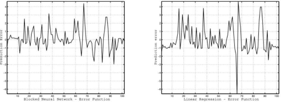
set. The cross validation performance (leave one out) of both models is shown

in figure 5 and figure 6. Especially by considering the error plots for each model

(see figure 6), one notices that the performance of the blocked neural network

is much better compared to the linear regression model. This observation is

confirmed by comparing the mean absolute errors, which is 0.8 for the blocked

neural network and 1.2 for the linear regression model. This means that the

neural network produces in the mean a prediction error of 0.8

major defects

per

document, compared to 1.2

major defects

for the linear regression model. Thus,

the nonlinear approach should be used to quantify the input output relationship

at the considered node. Based on the existing qualitative knowledge one would

expect that the performance of both models could be increased if the skipped

10 20 30 40 50 60 70 80 90 100 1 2 3 4 5 6 7 8 9 10

Blocked Neural Network − Cross Validation Performance 0.81143

No. of detected defects

10 20 30 40 50 60 70 80 90 100 1 2 3 4 5 6 7 8 9 10

Linear Regression − Cross Validation Performance 1.2316

No. of detected defects

Figure 5: Left: Performance of the blocked neural network. Right: Performance

of the linear regression model. Dashed line: Prediction. Solid line: Measurement

10 20 30 40 50 60 70 80 90 100 −6 −5 −4 −3 −2 −1 0 1 2 3 4

Blocked Neural Network − Error Function

Prediction Error 10 20 30 40 50 60 70 80 90 100 −6 −5 −4 −3 −2 −1 0 1 2 3 4

Linear Regression − Error Function

Prediction error

Figure 6: Left: Error between network prediction and measurement. Right:

Error between linear prediction and measurement.

variables like

human effects

,

complexity

or

familiarity with the product

were also

used as input variables of the models. The trained network function now can

be plugged into the simulation model and then can be used to determine the

number of detected major defects found in an inspection

during the simulation

runs.

Based on the trained blocked neural network we now compute and interpret

the partial derivatives and the relevance measures AD and AvE. The stability of

the calculated PDs for the considered neural network was proven by retraining

the neural network several times.

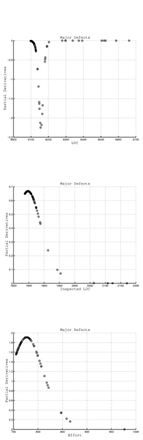
Figure 7 shows the plots of the partial derivatives of the variable

major

defects

with respect to all used input variables . One observes that the variables

whole range, while the variable

size of the product

only possesses negative

PD-values.

Considering the plot for the variable

effort

in more detail one notices that

for an actual effort in the range of 750 to 850 units increasing the effort while

leaving the remaining input variable unchanged leads to a significant increase

in the number of found defects. Obviously, the largest benefit for an increase

in the working effort in terms of additionally found major defects is obtained

around 775 units. An increase of the effort for documents with an actual value

already greater than 850 units only will lead to a slight increase in the number

of found defects, i.e. a saturation effect occurs. Thus, based on the PD-plot for

the variable effort and the known costs for each effort unit a software manager

approximately can determine the effort he would like to spend for the

inspec-tion. An analogous behavior of the partial derivatives can be observed for the

variable

inspected size of the product

. In contrast to the already considered

two input variables the explaining variable

size of the product

has negative or

zero partial derivatives. This means leaving the variable

effort

and

inspected

size of the product

unchanged and increasing the

size of the product

leads to a

smaller number of detected defects. One has to keep in mind that in this case

smaller percentage of the document will be inspected and that the effort and

the inspected lines of code are unchanged.

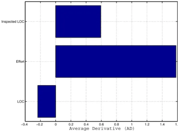
Figure 8 depicts of the AD-relevance measures (2) of the inputs, whereas

figure 9 displays the corresponding AvE-measures (see equation (3)). In both

figures one observes that the variable

effort

has the largest impact with respect

to the variable

detected major defects in the inspection

. As explained in the

last section the mean sign of correlation between the inputs and the output

can be determined by the AD-value, which is positive for the variables

effort

and

inspected size of the product

and negative for the variable

size of the product

.

All in all, the partial derivatives as well as the relevance measures contain

important quantitative information about the influence of the input variables

with respect to the considered output and thus provide the software manager

with a more detailed insight into the structure of the input output relation. He

especially gets able to estimate the impact of changes in the process.

In general the partial derivatives, the AD and AvE relevance measures also

can be used to validate a cause-effect diagram. Due to the lack of data this

aspect is not considered here in detail. In general the derived methodology

allows to check whether a variable is missing or redundant in the cause-effect

diagram, or if the signs indicating the direction of correlation between the input

and output are correct for the considered output node.

6000 6100 6200 6300 6400 6500 6600 6700 −2.5 −2 −1.5 −1 −0.5 0 Major Defects LOC Partial Derivatives 18000 1850 1900 1950 2000 2050 2100 2150 2200 0.1 0.2 0.3 0.4 0.5 0.6 0.7 Major Defects Inspected LOC Partial Derivatives 750 800 850 900 950 1000 0 0.2 0.4 0.6 0.8 1 1.2 1.4 1.6 1.8 2 Major Defects Effort Partial Derivatives

Figure 7: Plot of partial derivatives for the variable

Number of detected defects

in an inspection

with respect to the variables

size of the product

(top),

inspected

−0.4 −0.2 0 0.2 0.4 0.6 0.8 1 1.2 1.4 1.6 LOC

Effort Inspected LOC

Average Derivative (AD)

Figure 8: Plot of Average Derivative (AD)

0 5 10 15 20 25 30 35

LOC Effort Inspected LOC

Average Elasticity (AvE)

4

Conclusion

In this paper we have presented blocked neural networks as an appropriate tool

for quantification of static input output relationships of software development

processes. The performance of a blocked neural network with one neuron in each

block turned out to be superior compared to a linear regression model. The

major advantage of blocked networks compared to other nonlinear regression

models is the interpretability of the related partial derivatives and relevance

measures with respect to the impact of the single input variables. Plots of the

partial derivatives can be used to estimate the functional influence of each input

variable with respect to the output and thus can be used to find new rules of

thumb. They also can be used for validation of the existing qualitative models

of a software development process.

5

Acknowledgements

The authors gratefully acknowledge the support of this research done in

con-nection with the SEV project supported by the German Bundesministerium

f¨

ur Bildung und Forschung and the Prosim project supported by the Stiftung

Rheinlandpfalz f¨

ur Innovation, project no. 559.

References

[1] S. M. Carroll, B. W. Dickinson:

Construction of neural nets using the

Radon transform

. ’1989 IJCNN Proceedings.

[2] G. Cybenko:

Approximation by superpositions of sigmoidal functions

.

Math. Control, Signals, Systems, 2, 1989.

[3] B. Efron, R. J Tibshirani:

An Introduction to the Bootstrap

,

Mono-graphs on Statistics and Applied Probability 57, Chapman & Hall Inc.,

New York, 1993

[4] Ken-ichi Funahashi:

On the Approximate Realization of Continuous

Mappings by Neural Networks.

Neural Networks, 2(1989).

[5] Meihui Guo, Zhidong Bai, Hong Zhi:

Multi-Step prediction for

Non-linear Autoregressive Models Based On Empirical Distributions.

Sta-tistica Sinica 9(1999).

[6] J. M¨

unch, H. Neu, T. Berlage, T. Hanne, S. Nickel; S. Von Stockum;

A. Wirsen:

Simulation-based Evaluation and Improvement of Software

Developement Processes

,IESE-Report 048.02/E, August 2002

[7] H. Neu, T. Hanne, J. M¨

unch, S. Nickel, A. Wirsen:

Simulation

Based Risk Reduction for Planning Inspections

, Berlin, Springer

Inter-national Conference on Product Focused Software Improvement, 2002

Rovaniemi.

[8] T. Hastie, R. Tibshirani, J. Friedman:

The Elements of Statistical

Learning.

, Springer 2001

[9] K. Hornik, M. Stinchcombe, H. White:

Multileyer feedforward

net-works are universal approximators.

Neural Networks 2(1989).

[10] K. Hornik, M. Stinchcombe, H. White:

Universal Approximation of an

Unknown Mapping and Its Derivatives Using Multilayer Feedforward

Networks.

Neural Networks 3(1990).

[11] W. Y. Huang, R. Lippmann:

Neural Net and Traditional Classifiers

,

NIPS 1987.

[12] M. Lehtokangas, J. Saarinen, K. Kaski, P. Huuhtanen:

A Network

of Autoregressive Processing Units for Time Series Modeling.

Applied

Mathematics and Computation, 75, 1996.

[13] R. P. Lippmann:

An introduction to computing with neural nets

. ILEE

1987.

[14] B. M. P¨

otscher, I. R. Prucha:

Dynamic Nonlinear Econometric

Mod-els, Asymptotic Theory.

Springer 1997.

[15] P. N. Refenes, A. D. Zapranis, J. Utans:

Neural model identification,

variable selection and model adequacy.

Neural Networks in Financial

Engineering, Proc. NnCM-1996.

[16] A. Sarishvili:

Neural Network Based Lack Selection, for multivariate

time series

, Dissertation Universit”at Kaiserslautern, 2002

[17] Tschernig R, Yang LJ. :

Nonparametric lag selection for time series.

Journal of Time Series Analysis 21:(4) Jul 2000.

[18] H. White:

Learning in artificial neural networks: A statistical

perspec-tive.

Neural Computation 1(1989).

[19] Qiwei Yao, Howell Tong:

On subset selection in non-parametric

stochastic regression

Statistica Sinca 4(1994).

[20] Ning Xiong:

Designing Compact and Comprehensible Fuzzy

Con-trollers Using Genetic Algorithms

, Dissertation University of