Fast Point-Cloud Wrapping through Level-Set Evolution
Marco Marcon, Luca Piccarreta, Augusto Sarti, Stefano Tubaro Dip. di Elettronica e Informazione – Politecnico di Milano
Piazza L. Da Vinci 32 – 20133 Milano – Italy marcon/piccarre/sarti/[email protected] Abstract
In this paper we propose a fast algorithm for the reconstruction of surfaces from sets of unorganized sample points. The method is based on the temporal evolution of a volumetric function’s level-set derived from a PDE used in fluid dynamics. The reconstructed surface can be thought of as the front of a fluid that progressively fills up the space surrounding the cloud of points until it wraps them around. One interesting feature of this approach is its ability to model complex topologies using only properties such as fluid viscosity and vorticity. Another remarkable feature of this algorithm is its computational efficiency, which makes it suitable for interactive surface modelling [1]
1. Introduction
Modelling surfaces from unorganized sets of points, i.e., retrieving surface topology from surface geometry, is a long-debated problem in the computer vision community. When the point cloud is very dense and the surface topology is not so complex to generate topological ambiguities, a solution to this problem could be a simple Delaunay triangulation equipped with appropriate distance-based criteria. Point-connection ambiguities, however, are easy to arise even with dense data sets, and this is confirmed by a very rich literature on the topic.
In general, the solutions to the considered problem can be classified into two broad categories: those that directly construct the surface (boundary representation), and those that define the surface as a constraint in 3D space (volumetric representation). Working with boundary representations has the advantage of speed and allows us to control shape in a very straightforward fashion. Surface-based solutions, however, are difficult to use when dealing with complex topologies. Conversely, volumetric solutions tend to be quite insensitive to topological complexity (they may accommodate self-occluding surfaces, concavities, surfaces of volumes with holes, or even multiple objects), but they require a more redundant (volumetric) data structure, and a much heavier computational load.
One example of surface-based solution, proposed in [2,3], is based on the computation of the signed
Euclidean distance between each sample point and a linearly regressed plane that approximates the local tangent plane. The final surface is then obtained by interpolating this distance function with a marching cubes algorithm. Curless and Levoy [4] developed an algorithm tuned for laser range data, which is able guarantee a good rejection to point misalignments using the deviation from the local tangent plane. Another well-known approach is that of the α-shape [5,6], which associates a polyhedral shape to an unorganized set of points through a parameterised construction. Bajaj, Bernardini, and Xu [7] recently used the α-shape approach as a first step in a complete reconstruction pipeline. Finally, algorithms based on “Delaunay sculpting” are often used (see, for example, Boissonnat [8] and Amenta ed al. [9]). Such solutions progressively eliminate tetrahedra from the Delaunay triangulation based on their circumspheres.
Algorithms based on the temporal evolution of an initial curve towards the boundary of the structure of interest turned out to be significantly improved by the introduction of the snake model presented by Kass, Witkin and Torzopoulos, in which an initial surface evolves in such a way to minimise a properly defined potential (cost function) [10]. The snake model was the origin of a significant number of mathematical formulations that have been used in imaging, vision and graphics during the past 15 years. Such techniques are implicit, intrinsic and can deal with topological changes that may occur while tracking moving interfaces.
Level-set techniques are currently becoming more and more popular for various types of applications ranging from the modelling of physical phenomena such as the propagation of interfaces in crystals and gasses, image processing, volume modelling, etc. These methods were introduced in parallel by Osher and Sethian [1]. People in imaging, begun using such techniques at the beginning of the 90s [11,12] and they have now become an established area of research in vision and graphics as well.
Level-set techniques belong to the category of volumetric surface modelling solutions and require a volumetric function to be updated at every time step until the evolving front (level-set) reaches the desired configuration. If the volumetric function is defined on a voxset of N voxels per side, in principle the evolution
requires an order of N3 voxels to be updated for a
number of iterations that is proportional N. This number of updates can be reduced from an order of N4 to an
order of N3 by limiting the volume of interest to a narrow
band surrounding the evolving front [1]. More recently, a multi-resolution approach to level-set evolution was proposed in order to further reduce the number of updates to an order of N2 log N [13]. Still, all such
solutions need further steps to sufficiently reduce the computational cost and bring volumetric methods to practical usability.
In this paper we propose a novel approach to level-set evolution that dramatically reduces the computational cost of the method down to the level of surface-based solutions. In order to do so, we adopt a model for the time-space evolution of the level-set based on the Navier-Stokes equations [14], which provide us the most general description of a fluid flow.
Typically a level-set equation involves a velocity field v that depends on the geometry of the zero level set and external quantities that can be thought of as depending on x and t. A prototype of this equation is:
( )
( )
a
ϕ
µ
ϕ
ϕ
ϕ
⎛
⎞
∇
∇
=
∇
−
∇⋅⎜
⎜
∇
⎟
⎟
⎝
⎠
v
x
x
where ϕ represents the volumetric function whose level-set zero is the evolving shape, a(x) represents the convection (in the normal direction) and µ(x) is the curvature-dependent motion. The presence of the implicit function in the velocity field forces us to update the velocities at each time step. This operation is, indeed, computationally demanding and, although a wide variety of methods exist for speeding it up, it constitutes a bottleneck for level-set equations based on the Hamilton-Jacobi PDEs.
Using a completely different PDE allows us to compute the velocity field only once in an initialization phase of the level-set. During this phase the fluid evolution is oriented towards the nearest sample point. In addition, in order to guarantee a fast evolution and a smooth convergence, its speed is proportional to the distance from the nearest point.
The method that we propose further improves the ability of level-set methods to adapt to complex topological configurations using an advanced physical description of the fluid behaviour, which includes viscosity and vorticity.
2. The fluid evolution paradigm
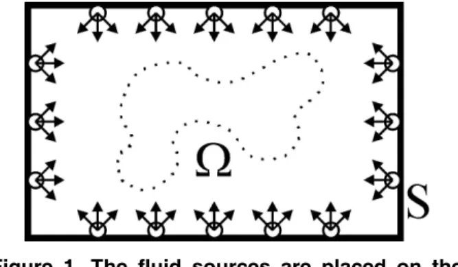
Our level-set evolution describes a fluid flowing in a region Ω, which is chosen in such a way to include the cloud of points. As shown in figure 1 the fluid is generated by sources placed on the boundary S of that region, and it stops when all the space outside the cloud of sample points is filled up. A volumetric function F is defined in such a way to describe the amount of fluid that is in each voxel.
Figure 1. The fluid sources are placed on the boundary of the voxset. The fluid flows from there towards the cloud of points until it fills of the space outside them.
It F = –1 at a specific voxel, then that voxel is considered as empty. If, on the other hand, F=1, then that voxel is interpreted as entirely filled up with fluid. Intermediate values of F tell us how much fluid is present in the voxel. This information gives us a precise indication of where the front is within the voxel. In fact, using the values of F in a neighbourhood of the considered voxel we can localise the front with sub-voxel resolution using, for example, a simple marching cubes algorithm. The front of the moving fluid is identified by the zero level-set of the function F, which is the surface that eventually will wrap the cloud of points.
At the beginning of the system evolution all the space is empty and each voxel is set to a conventional value of – 1. The external fluid sources are placed only on the region boundary, and they are simply modelled as voxels whose value is kept steadily at the value +1. From this initial condition the system is left free to evolve while following an equation based on the Navier-Stokes model for the conservation of the mass with a redefinition of the speed vector v as defined below.
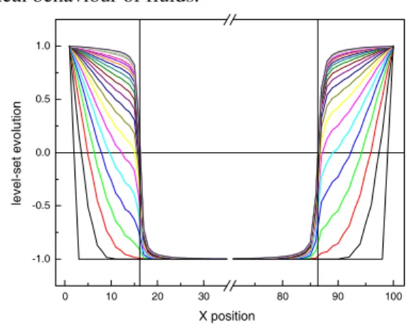
In Figure 2 we show the evolution of the fluid front in a one-dimensional case. The cloud of points is here represented by the sole two points located at x1=16.3 and
x2=86.4. The fluid originates from the boundary and
flows inward filling up the space until it reaches the two points. The level-set zero of the implicit function will enevtually correspond exactly to the two points. Using this fluid dynamics model is then possible to implement a fast algorithm that fills up the whole space outside the cloud of points, leading to a smooth surface that wraps it.
The law of mass conservation is a general statement of kinematic nature that does not depend on the nature of the fluid or on the forces that act on it. This law expresses the empirical fact that, in a fluid system, mass can neither disappear from the system nor be created except in sources or drains.
The volumetric function F describes the specific mass of the fluid. The general form of conservation law for a system bounded by a closed surface S can be expressed in terms of the variations of F due to the fluxes and the sources Q. The flux vector G represents the amount of fluid orthogonally crossing an infinitesimal surface element dS per time unit. This vector has two
components, a diffusive contribution GD and a
convective part GC, both of which characterize the
physical behaviour of fluids.
0 10 20 30 80 90 100 -1.0 -0.5 0.0 0.5 1.0 le ve l-se t e vol ut io n X position
Figure 2. Level-set evolution for a 1D case. At the end the fluid fills up the whole space outside the two points x1=16.3 and x2=86.4.
In its general form, a conservation law states that the variation of F per time unit within the volume Ω is
Fd
t
Ω∂
∂
∫
,which is equal to the net contribution from the sources and the incoming fluxes through the external surface S,
S
d
⋅
∫
G S
,where the surface element vector dS points towards the inside of the region.
These sources can be divided into isotropic volume sources Qv and oriented surface sources QS . The total
contribution is V S S
Q d
d
Ω⋅
+
⋅
∫
∫
4
6
.Notice that surface sources are oriented and their net contribution depends from orientation of surface element vector dS. In conclusion, the general form for the conservation equation of the quantity F is
V S S S
Fd
d
Q d
d
t
Ω Ω∂
=
⋅
+
⋅
+
⋅
∂
∫
∫
* 6
∫
∫
4
6
or, using Gauss’ theorem for continuous fluxes and surface sources, we obtain
V S
Fd
d
Q d
d
t
Ω Ω Ω Ω∂
= ∇ ⋅
+
+ ∇⋅
∂
∫
∫
*
∫
∫
4
.This last equation leads to the differential form of the conservation law, as it holds true for an arbitrary volume Ω: V S
F
Q
t
∂ = ∇⋅ + +∇⋅
∂
G
Q
.A crucial aspect of the conservation law is that the internal variations of F, in the absence of volume
sources, depend only on the flux contribution through the surface S and not on the flux values inside the volume Ω.
Separating the flux vector into its two convective and diffusive components, GC and GD, we obtain a more
detailed form of the equation. Indeed the convective part of the flux vector GC, attached to the quantity F in a flow
of velocity v is the amount of F transported with the motion, and is given by
G
C=
v
F
.The diffusive flow is defined as the contribution present in fluids at rest; it is due to the molecular, thermal agitation and is usually proportional to the gradient of F, i.e.
G
D= ∇
γ
F
,where γ is the diffusivity constant.In our algorithm we oriented the velocity v for the propagation of the fluid towards the nearest sampled point. Each point, therefore, represents an attractor for it. The modulusof the velocity vector is proportional to the distance from the nearest point, which allows the fluid to gently converge to the desired surface. A further diffusive behaviour is also taken into account to obtain a more natural flux and a smooth interpolating surface.
We joined together the two contributions of the flux defining the convective part as above and implementing the diffusive part weighting the contributions from the near points with a Gaussian function: this is the classical result of the thermal diffusion PDE. With this IRUPXODWLRQWKHVWDQGDUGGHYLDWLRQ LQHTXDWLRQSOD\V a role similar to the diffusivity term γ.
Following the previous statements we propose the equation (1) for the temporal evolution of the implicit function F
( )
2 2 2 2 2 2( ) ( )
( )
( )
F
e
d
F
F
t
e
d
σ σ − − Ω − − Ω∂
=
−
∂
∫
∫
x w x ww v w
w
x
x
v w
w
(1)Experimentally we found that a sharp square function that extends only to the 6 nearest neighbours (for the 3D case) works as well as the Gaussian weighting function, and this is particularly useful for discretizing eq. (1). The discretized version of the eq. (1) that we used is given in eq. (2) ( , ) ( , ) ( , 1) ( , ) ( , ) i i j j j i i i i j j F t v w F t v F t F t F t v w v + + − = − +
∑
∑
x x x x x i.e.: ( , ) ( , ) ( , 1) i i j j j i i j j F t v w F t v F t v w v + + = +∑
∑
x x x , (2)where the summation j extends over the nearest neighbour of x as shown in Figure 3, w represent the smoothing (diffusive) term and its value may vary from 0.1 to 0.9. Using the fluid dynamics terminology w
represents the viscosity of the fluid that we are considering.
Figure 3. The six nearest neighbour for a 3D voxset
Viscosity is an internal property of a fluid that describes its resistance to flow. Accounting for it prevents interstitial flow inside the object where sparse samples are present. It also reduces the curvature of the whole surface giving a smooth final surface. The curvature in a 2D case, for example, can be monitored through an energy functional defined as
2
( ) 2
2( )
2( )
xx xy yy
E
f
f
f
d
Ω
=
∫
x
+
x
+
x x
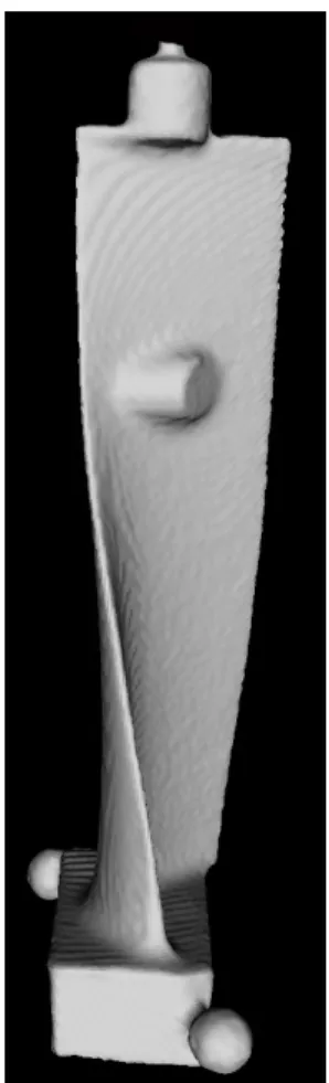
. The lower the value of E the smoother the surface even with a low point-cloud density [15]. Figure 4 shows a good reconstruction of a sharp blade of an airscrew that proves the effectiveness of our algorithm in situations where traditional level-set solutions usually fail.In order to speed up computations, only the voxels where the derivative of the F(x)exceeds a threshold are recomputed at every time step, while all the others are kept fixed. In (1)
v x
( )
is defined asx p
−
α where p is a vector indicating the nearest point to x while α adjusts the speed of convergence (good values of α are typically in the range between 1.6 and 2.4). Unlike traditional level-set algorithms, our approach always defines the distance as a positive number (α = 2), which results in a faster evolution (farther points are assigned a greater speed) and a more accurate convergence near the desired surface configuration.3. The vorticity equation
Another important physical phenomenon of fluid dynamics that turns out to be quite useful for our purposes is the vorticity, which describes the presence of turbulence in the motion of fluids. Its introduction allows us to describe local variations in the velocity term and to localize whirls. Their behaviour is defined by a rotational component in the velocity vector field
( )
= ∇×
Y [
.The intensity of this vector characterizes the turbulence. The rotational behaviour can be illustrated by defining an imaginary loop C around the whirl and then integrating the flow velocity around that loop: we found that the resulting number is not necessarily zero.
C
Γ =
∫
v dl
⋅
.Figure 4. A sharp blade of an airscrew, model obtained from a cloud of 1,550,316 points in a voxelset of 180 voxels per side, the image shows the viscosity contributtion
Applying Stokes’ theorem to this equation we obtain
(
)
C S S
Γ =
∫
v dl
⋅ = ∇
∫
× v dS
⋅
=
∫
⋅
G6
, where the right-hand integration is extended throughout the surface S defined by the closed loop C. In conclusion, the vorticity represents the local rotational aspect of the flow.The presence of whirls can locally develop high-pressure gradients and may generate instabilities in the flow but, at the same time, it can favour penetration inside narrow openings and prevent fluid from stagnating in ‘low speed’ regions. Although the localization of vortices and the determination of their intensity is quite a difficult numerical problem, it is impossible to neglect them if we want to correctly model our system.
In our solution we artificially introduce the presence of vortices by modulating the velocity field with small oscillations around the initial configuration. Due to the close correlation between the velocity vector and the vector pointing toward the nearest point (see the previous section) the modulation in the velocity field can also be interpreted as a plastic deformation of the sample cloud of points in the various directions. Roughly speaking, this operation is similar to that of forcing jello through a funnel by squeezing the funnel itself.
The modulation of the velocity function is obtained by cycling through the three spatial axes the direction of expansion. More specifically, at each step we multiply the velocity component in the expansion direction for an assigned coefficient while we shrink the other two components of the vector dividing them for the same factor. We founded that good values for the expansion coefficient range from 1 to 1.5. Larger values may result in an undesired behaviour, such as having repulsion of the fluid from the surface.
Figure 5. The introduction of vorticity allows us to honor also difficult topologies like the dragon’s mouth
4. Improving the accuracy
As already explained above, the whole volume is initialized with the value -1 indicating the total absence of fluid with the exclusion of the boundary of the voxel set where we placed the fluid sources. This approach gives a good approximation of the desired surface as the fluid moves towards the cloud of points but may require a long time in particularly complex topologies involving deep and narrow concave surfaces. In this case the user can add sources of the fluid near these structures improving the converging time.
Another issue to obtain a better reconstruction is obtained by near-source local relaxation: sources that are placed too close to sample points can prevent a correct reconstruction of the surface. In fact, an excessive flow of fluid could result in an overflow through the desired surface. In order to overcome this problem, we monitor the gradient of the front near the level-set zero: if it exceeds an assigned threshold, then the intensity of the source is reduced in such a way to improve the match with the location of the sample points. One way to avoid this problem is to use a larger voxel-set at the cost of a heavier resource usage. Another possible solution is obtained calibrating the intensity of the sources near the cloud of points
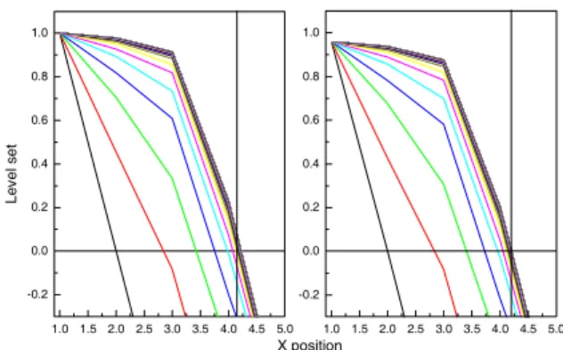
In Fig. 2 we show the evolution of the system in a 1D environment, we placed two points, at x=16.3 and x=86.4, placed in a space of 100 points. Their position is correctly honoured from the level-set evolution as long as they are far from the boundary. In Fig. 6 we can see the evolution of a level-set when the point is very close to the volume boundary and the external fluid overflows pushing the level-set zero inside (the point is placed at x = 4.2). 1.0 1.5 2.0 2.5 3.0 3.5 4.0 4.5 5.0 -0.2 0.0 0.2 0.4 0.6 0.8 1.0 Le ve l s et X position 1.0 1.5 2.0 2.5 3.0 3.5 4.0 4.5 5.0 -0.2 0.0 0.2 0.4 0.6 0.8 1.0
Figure 6. Undesired overflow of the external source (left) and its correction reducing the source strenght (right).
5. Multi-region approach
In addition to the above-described advantages our algorithm can be easily parallelized and different parts of the cloud of points can be separately rendered on different threads or different processors with different resolutions. When all the single parts have converged to the final solution, they can be easily merged together on a voxset that is able to accommodate the various parts. The resolution of this voxset will correspond to the highest resolution of the components. In order to smoothly merge the various parts, it is important to make sure that the regions are partially overlapped. After re-tiling the regions in the proper position, we perform volumetric merging by constructing the overall volumetric function as
( )
inf
i( )
i
F
x
=
F
x
where the inf operator acts wherever the implicit functions overlap. This corresponds to using a greyscale morphological operator that returns the union of the two regions. In Figure 7 we illustrate this approach for a 2D case: the three overlapping zones are separately rendered and then they are merged using the previously-described operator.
6. Conclusions
The new fluid dynamic model for the level set evolution has been implemented in 2D and in 3D. One remarkable feature of the algorithm is its speed. This is proved by the rendering times for some well-known data sets, which are reported in Table 1 for several resolution levels. Various implementational issues have been adopted in order to boost the performance of the proposed algorithm. For example, we perform a pre-computation of the speed vector field for each voxel and we developed an efficient freezing algorithm for voxels that are no longer involved in the front propagation.
As far as the 3D algorithm is concerned the updating is obtained by moving from the most external box towards the central point of the space; the update is then
performed in concentric boxes following a Chinese-boxes path.
Figure 7. Volumetric merging of individually computed level-set regions.
In Figure 8 there is the representation of the level sets for a circle made of 50 point with a radius of 30 points, The time required for the convergence is 3 s.
The level set evolution in 3D is reported for the different sets of points. In Table 1 we list the computational time required for rendering the sets of points represented in Figs. 4, 9 and 11. The rendering was performed on a AMD Athlon™ XP at 2.1 GHz with 512 MB RAM under Windows™ 2000.
Figure 8. 2D rendering of a circle (initial pixel-set of 50 pixels per side, radius of 30 pixels). Synthetic point data-set.
The Wolf, the Teapot and the Airscrew are interesting data-sets because they allow us to test the method on slightly noisy data acquired from different sources.
The resulting mesh is obtained by the marching cube algorithm.
An example of surface wrapping based on local reconstruction followed by volumetric merging is shown in Figure 11 for the rabbit data set. We divided the data
set in 3 partially overlapping portions, and we re-assembled their volumetric function as shown in figure 10.
Set Resolution Points Time (s)
Bunny 1803 35780 40
Bunny 1003 35780 4
Happy buddha 3503 3836 105
Teapot 2563 33061 110
Airscrew 3003 1550316 120
Table 1. Computational time of the 3D algorithm, the resolution in the maximum number of points along the larger dimension of the object.
In this paper we proposed a novel volumetric approach to surface modeling from unorganized sets of points, which is able to overcome the typical problems of computational efficiency of level-set methods. In addition, we gave the algorithm the ability to model complex topologies using advanced fluid-dynamics properties of fluids.
The results in terms of both computational efficiency and topological flexibility are very encouraging, and make the approach extremely usable.
Figura 9. The level-set evolution for the wolf data-set.
Figura 11. Other examples
References
[1] J.A. Sethian, Level Set Methods and Fast Marching Methods Evolving Interfaces in Computational Geometry, Fluid Mechanics, Computer Vision, and Materials Science, Cambridge University Press, 1999
[2] H.Hoppe, T.DeRose, T.Duchamp, J.McDonald, W.Stuetzle. Surface Reconstruction from Unorganized points in SIGGRAPH’92 Proceedings, pages 71-78, July 1992
[3] H. Hoppe. Surface Reconstruction from Unorganized Points. Ph.D. Thesis, Computer Science and Engineering, University of Washington, 1994.
[4] B. Curless and M. Levoy. A volumetric method for building complex models from range images. In SIGGRAPH
’96 Proceedings, pages 303–312, July 1996.
[5] H. Edelsbrunner, D.G. Kirkpatrick, and R. Seidel. On the shape of a set of points in the plane, IEEE Transactions on
Information Theory 29:551-559, (1983).
[6] H. Edelsbrunner and E. P. Mücke. Three-dimensional Alpha Shapes. ACM Transactions on Graphics 13:43–72, 1994.
[7] C. Bajaj, F. Bernardini, and G. Xu. Automatic reconstruction of Surfaces and Scalar Fields from 3D Scans.
SIGGRAPH ’95 Proceedings, pages 109–118, July 1995.
[8] J-D. Boissonnat. Geometric structures for three-dimensional shape reconstruction, ACM Transactions on
Graphics 3: 266–286, 1984.
[9] Nina Amenta, Marshall Bern and David Eppstein. The Crust and the Skeleton: Combinatorial Curve Reconstruction. To appear in Graphical Models and Image Processing. [10] M.Kass, A.Witkin, D.Terzopoulos. Snakes: Active contour Models. In IEEE International Conference in Computer Vision, pages 261-268, 1987.
[11]V.Caselles, F.Cattè, B.Coll, F.Dibos. A geometric model for active contours in image processing, Numerische
Mathematik, 66(1):1-31,1993
[12]R. Malladi, J.Sethian and B.Vemuri. Evolutionary fronts for topology independent shape modelling and recovery. In
European Conference on Computer Vision, Pages 1-13, 1994
[13] A. Sarti, S. Tubaro: "Image-Based Multresolution Implicit Object Modeling". J. on Applied Signal Processing, Vol. 2002, No. 10, Oct. 2002, pp. 1053-1066.
[14] C.Hirsh, Numerical computation of internal and external flows, (Wiley interscience series in numerical methods in engineering;1) ISBN 0471917621
[15] Greg Turk and James F. O'Brien. "Shape Transformation Using Variational Implicit Functions." The Proceedings of
ACM SIGGRAPH 99. Los Angeles, California, August 8-13,