University of Pennsylvania
ScholarlyCommons
Publicly Accessible Penn Dissertations
2017
Essays On Banking
Eric Moore
University of Pennsylvania, [email protected]
Follow this and additional works at:https://repository.upenn.edu/edissertations
Part of theFinance and Financial Management Commons, and thePublic Policy Commons
This paper is posted at ScholarlyCommons.https://repository.upenn.edu/edissertations/2483 For more information, please [email protected].
Recommended Citation
Moore, Eric, "Essays On Banking" (2017).Publicly Accessible Penn Dissertations. 2483.
Essays On Banking
Abstract
In the first chapter, I use a fuzzy regression discontinuity design to study the impact of auction-based emergency liquidity at the onset of the 2007-09 crisis. My empirical design uses the presence of binding auction capacity constraints to isolate variation in short-term borrowing from the Federal Reserve. I find that the growth in marginal winners' outstanding loan commitments is about 15% higher than marginal losers. This effect stems through more lending: marginal winners' loan growth was about 8% higher than that of marginal losers. These effects arise despite the ability to replicate this auction-based liquidity's funding structure through the discount window. They highlight that banks would have relied considerably less on the Federal Reserve had only the discount window been in place during the crisis. I discuss the role of discount window stigma in partly explaining these results.
In the second chapter, I study the relationship between confidentiality and contract enforcement. I specifically examine whether publicly exposing past-due borrowers increases their lenders' propensity to seek loan recovery through the legal system. I explore this question in the context of a large rise in past-due loans within India's government-owned banks, which led a bank employees' association to disclose the largest defaulters' identities and loan amounts. Overall, this group increased the probability of legal enforcement by about 10%, with most of this effect arising from their initial threat to expose these defaulters. Lenders targeted past-due borrowers that could likely have avoided default, which is consistent with a desire to reduce the perception of corruption that might follow from disclosure.
Degree Type Dissertation Degree Name Doctor of Philosophy (PhD) Graduate Group Applied Economics First Advisor Santosh Anagol Keywords
Contract Enforcement, Discount Window, Emergency Liquidity Provision, Financial Crisis, Information Disclosure, Term Auction Facility
Subject Categories
ESSAYS ON BANKING Eric Moore
A DISSERTATION in
Applied Economics
For the Graduate Group in Managerial Science and Applied Economics Presented to the Faculties of the University of Pennsylvania
in
Partial Fulfillment of the Requirements for the Degree of Doctor of Philosophy
2017
Supervisor of Dissertation _____________________
Santosh Anagol, Assistant Professor of Business Economics and Public Policy
Graduate Group Chairperson ______________________
Catherine Schrand, Celia Z. Moh Professor, Professor of Accounting Dissertation Committee:
Santosh Anagol, Assistant Professor of Business Economics and Public Policy Michael Roberts, William H. Lawrence Professor, Professor of Finance
ABSTRACT ESSAYS ON BANKING
Eric Moore Santosh Anagol
In the first chapter, I use a fuzzy regression discontinuity design to study the impact of auction-based emergency liquidity at the onset of the 2007-09 crisis. My empirical design uses the presence of binding auction capacity constraints to isolate variation in short-term borrowing from the Federal Reserve. I find that the growth in marginal winners’ outstanding loan commitments is about 15% higher than marginal losers. This effect stems through more lending: marginal winners’ loan growth was about 8% higher than that of marginal losers. These effects arise despite the ability to replicate this auction-based liquidity’s funding structure through the discount win-dow. They highlight that banks would have relied considerably less on the Federal Reserve had only the discount window been in place during the crisis. I discuss the role of discount window stigma in partly explaining these results.
In the second chapter, I study the relationship between confidentiality and contract enforcement. I specifically examine whether publicly exposing past-due borrowers increases their lenders’ propensity to seek loan recovery through the legal system. I explore this question in the context of a large rise in past-due loans within India’s government-owned banks, which led a bank employees’ association to disclose the largest defaulters’ identities and loan amounts. Overall, this group increased the probability of legal enforcement by about 10%, with most of this effect arising from their initial threat to expose these defaulters. Lenders targeted past-due borrowers that could likely have avoided default, which is consistent with a desire to reduce the perception of corruption that might follow from disclosure.
TABLE OF CONTENTS
ABSTRACT . . . iii
LIST OF TABLES . . . v
LIST OF FIGURES . . . vi
CHAPTER 1: Auction-Based Liquidity of Last Resort . . . 1
1.1 Introduction . . . 2
1.2 Liquidity Provision by the Federal Reserve . . . 7
1.3 Data & Empirical Design . . . 16
1.4 Results . . . 27
1.5 Discussion . . . 34
1.6 Tables & Figures . . . 36
CHAPTER 2: Stakeholder Governance and the Threat of Disclosure . . . . 56
2.1 Overview . . . 57 2.2 Institutional Background . . . 63 2.3 Data . . . 77 2.4 Empirical Design . . . 79 2.5 Results . . . 83 APPENDIX . . . 94 BIBLIOGRAPHY . . . 113
LIST OF TABLES
TABLE 1 : Auction Characteristics . . . 37
TABLE 2: Bidder Characteristics . . . 38
TABLE 3: Bank Characteristics and Proximity to the Stop-Out Rate . . . 39
TABLE 4: Marginal Losers’ Probability of Bidding in the Next Auction . . 40
TABLE 5: Term Auction Facility Borrowing at the Stop-Out Rate . . . 41
TABLE 6: Balance of Pre-Determined Characteristics . . . 42
TABLE 7: Outstanding Loan Commitment Growth at the Stop-Out Rate . 43 TABLE 8: Fuzzy RDD Estimates of the Term Auction Facility’s Impact . . 44
TABLE 9: Fuzzy RDD Estimates by Loan Type . . . 45
TABLE 10: Results when the Stop-Out Exceeds the Discount Rate . . . 46
TABLE 11: Summary of India’s Public-Sector Banks . . . 66
TABLE 12: Public-Sector Banks Relative to Other Banks . . . 68
TABLE 13: The Largest Defaulters within India’s Public-Sector Banks . . . 71
TABLE 14: AIEBA’s Impact on Default Disclosure . . . 73
TABLE 15: Listed Top Defaulters’ Bank Relationships in 2013Q1 . . . 78
TABLE 16: Example of Cranes Software’s Default . . . 82
TABLE 17: Impact of Disclosure on Legal Enforcement . . . 84
TABLE 18: Impact of Disclosure by Legal Enforcement Type . . . 90
TABLE 19: Effect on Legal Enforcement Based on Shareholders’ Equity . . 91
TABLE A.1: Other Treatment Measures at the Stop-Out Rate . . . 105
TABLE A.2: Fuzzy RDD Estimates Including a Past Borrower Control . . 106
TABLE A.3: Fuzzy RDD Estimates with All Over-Subscribed Auctions . . 107
TABLE A.4: Fuzzy RDD Estimates Using Raw Rank . . . 108
TABLE A.5: List of Public Sector Banks in India . . . 109
TABLE A.6: Summary of Bank Ownership Variables . . . 110
TABLE A.7: Remaining Defaulters in Initial Disclosure . . . 111
LIST OF FIGURES
FIGURE 1: TED Spread During the Early Stages of the Crisis . . . 47
FIGURE 2: Summary of Auction Capacity Constraints . . . 48
FIGURE 3: Probability that Loan Request is Accepted in an Auction . . . 49
FIGURE 4: Probability of TAF Loan by the Quarter End . . . 50
FIGURE 5: Balance of Pre-Determined Bank Characteristics . . . 51
FIGURE 6: Aggregate Lending Around Sample Period . . . 52
FIGURE 7: Outstanding Commitment Growth Prior to Sample . . . 53
FIGURE 8: Commitment Growth Around the Stop-Out Rate . . . 54
FIGURE 9: Comparison of Stop-Out and Discount Window Rates . . . 55
FIGURE 10: Non-Performing Loans in India’s Commercial Banks . . . 64
FIGURE 11: Legal Enforcement Against Top Defaulters . . . 76
FIGURE 12: Lack of Pre-Trends in Legal Enforcement . . . 87
FIGURE 13: Robustness to Excluding Individual Firms . . . 89
FIGURE A.1: Foreign Banks by Raw Bid Rank . . . 95
FIGURE A.2: Other Measures of TAF Borrowing at the Stop-Out Rate . . 96
FIGURE A.3: Fuzzy RDD Estimates with First-Order Polynomial . . . 97
FIGURE A.4: Fuzzy RDD Estimates with Second-Order Polynomial . . . . 98
FIGURE A.5: Non-Performing Loans in India’s Banks (2008 - 2015) . . . . 99
FIGURE A.6: Write-Offs in India’s Commercial Banks (2008 - 2013) . . . 100
FIGURE A.7: New Corporate Debt Restructuring Mechanism Cases . . . 101
FIGURE A.8: Value of Corporate Debt Restructuring Mechanism Cases . 102 FIGURE A.9: Ownership Summary of India’s Commercial Banks . . . 103
Chapter 1: Auction-Based Liquidity of Last Resort
Eric Moore
Abstract
I use a fuzzy regression discontinuity design to study the impact of auction-based emergency liquidity at the onset of the 2007-09 crisis. My empirical design uses the presence of binding capacity constraints in the Federal Reserve’s Term Auction Facility to isolate variation in short-term borrowing through this program. I find that the growth in marginal winners’ outstanding loan commitments is about 15% higher than marginal losers. This effect stems through more lending: marginal winners’ loan growth was about 8% higher than that of marginal losers. These effects arise despite the ability to replicate this auction-based liquidity’s funding structure through the discount window. They highlight that banks would have relied considerably less on the Federal Reserve had only the discount window been in place during the crisis. I discuss the role of discount window stigma in partly explaining these results.
1.1 Introduction
Inter-bank lending markets help ensure an efficient allocation of capital in the banking system. While these markets facilitate re-allocating surplus liquidity in nor-mal times, potential lenders may hoard liquidity during a financial crisis and, thereby, force banks in need of funding to cut lending. Central banks should provide liquidity in such circumstances, but banks may under-utilize such funding as their borrow-ing, if discovered by market participants, could provide a negative signal about their credit-worthiness. In light of these concerns, one approach taken during the crisis was to adjust how short-term funding was provided directly to banks. One of the Federal Reserve’s early responses to the 2007-09 crisis was to create auctions for emergency liquidity. This raises a simple question: How much does the nature of emergency liquidity matter?
This question is challenging to answer for two reasons. First, it is difficult to find a valid counterfactual for banks that utilize emergency funding. These banks are likely to differ along unobservable dimensions, implying that a regression of bank lending on emergency liquidity suffers from an omitted-variable bias. Second, assuming this challenge were overcome, one would still need to contrast the effect of one approach relative to a close, but distinct, alternative to highlight how much that funding’s characteristics ultimately mattered.
Quantifying the impact of different ways to provide short-term loans is important given the key role that such changes played in the early response to the 2007-09 finan-cial crisis. In 2007, for example, the Federal Reserve established the Term Auction Facility, an auction-based approach to granting short-term funding to banks that sub-stituted for pre-existing funding available through the discount window. With over $3.8 trillion in Term Auction Facility loans granted, this program was an apparent success at encouraging banks to borrow, but its impact on bank lending is unclear.
Much of this borrowing might have occurred with only the discount window in place during the crisis. Banks can also hoard liquidity, suggesting that banks might borrow but not expand credit to borrowers.1
I propose an empirical strategy to estimate the impact of the Term Auction Fa-cility that utilizes the presence of binding capacity constraints in these auctions. Specifically, I leverage over $600 billion in loan requests that were not granted by comparing the outcomes of banks with bids placed close to, but on either side of the market-clearing interest rate in each auction. As most marginal losers pursue fund-ing again through future auctions, I use failure to obtain fundfund-ing in a given auction as an instrument for future borrowing in the same quarter within a fuzzy regression discontinuity design.
I focus on the impact on banks’ outstanding loan commitments. Loan commit-ments are contractual obligations to provide funding. They are an important source of liquidity and play a key role in our understanding of banks. In the seminal model of Kashyap, Rajan, and Stein (2002), banks provide liquidity to borrowers through loan commitments. In providing this liquidity, banks must hold liquid assets to help fund unpredictable drawdowns. Liquidity pressures can thus damage banks’ ability to commit new funding to borrowers. As loan commitments account for around 80 percent of all commercial and industrial loans alone, they are a key channel through which illiquidity can affect the economy.2
Outstanding commitments specifically measure the “unused” component of banks’ loan commitments. Defined in this manner, this variable will increase if banks grant more loans but also if borrowers arrest drawdowns on pre-existing lines of credit. I find that Term Auction Facility funding increased the growth in outstanding
com-1A variety of models of the inter-bank market can feature banks hoarding liquidity in equilibrium.
For example, see Allen, Carletti, and Gale (2009) and Heider, Hoerova, and Holthausen (2015). Freixas and Jorge (2008) provide a model of the interbank market with credit rationing.
mitments: this growth rate was 15% larger for marginal winners than marginal losers when considering banks’ whose highest bid fell within the vicinity of the market-clearing interest rate.3 This result i) is not present prior to the establishment of the Term Auction Facility, ii) is robust to different bandwidth and polynomial choices and iii) is not explained by discontinuous changes in bank characteristics at the market-clearing interest rate.
This result alone illustrates that auction-based liquidity through the Term Auction Facility was important despite the co-existence of discount window funding. It does not, however, indicate specifically whether the effect comes from more lending or reduced drawdowns on pre-existing commitments. One can gauge which is at work by looking at a comprehensive credit growth measure that includes on-balance sheet loans and off-balance sheet commitments. This outcome would move in response to loan supply changes, but not from borrowers’ drawdowns. Consistent with a loan supply interpretation, the growth in this comprehensive measure was about 6-8% higher for marginal winners relative to marginal losers.
Understanding why this result exists is important considering there is a proposal in the U.S. Congress that would require the Federal Reserve to immediately disclose its borrowers’ solvency.4 Bernanke (2015) highlights that this could eliminate the Federal Reserve’s ability to provide emergency liquidity by making banks become unwilling to borrow from the Federal Reserve altogether, i.e. the stigma problem. While the existence of this stigma is well-established, e.g. see Armantier et al. (2015), its broader consequences are largely unknown.
Stigma might explain my results as all Term Auction Facility bidders could borrow at the Federal Reserve’s discount window, which grants similar loans on ano questions
3Section 1.3.1 discusses why I focus on banks’ highest bids.
4The specific legislative proposal is S. 1320, also called the “Bailout Prevention Act of 2015”
(Congress (2015)). It was introduced into the Senate on May 13th, 2015 by Senators Elizabeth Warren (D-Massachusetts) and David Vitter (R-Louisiana).
asked basis. If a bank fails to receive a Term Auction Facility loan, it can often replicate the same funding structure through the discount window.5 Differences in outcomes between marginal winners and losers suggest a stigma-based explanation, but they might also arise as Term Auction Facility loans were at times less expensive than the discount window. Which mechanism is at work provides insight into the consequences of requiring the Federal Reserve to disclose its borrowers’ solvency.
To test the stigma-based explanation, I examine the lending effect in the sub-sample where the auctions were more expensive than the discount window. During these auctions, a bank whose bid was marginally below the auction’s market-clearing rate could have immediately borrowed at the discount window at a relatively lower interest rate. Should the lending effect arise in this sub-sample, then a stigma-based explanation is merited. Conversely, when the market-clearing interest rate in the auction is below the discount window rate, banks might lend more because they have access to a cheaper funding source.
I show that my main result is similar in magnitude in this sub-sample. This suggests that some banks may have placed a bid above the discount window rate that fell below the auction market clearing rate ex post, but were not willing to subsequently replicate their loan request through the discount window. In effect, it suggests that banks were willing to take loans through the auctions that they were not willing to take through the discount window simply because of stigma.6 Auction-based liquidity appears, in part, to stimulate borrowing that would never
5My sample includes the 21 capacity constrained auctions where a borrower could essentially
replicate the Term Auction Facility funding structure at the discount window. The other two of the 23 auctions with a binding capacity constraint granted 84-day maturity loans and so a borrower could not fully replicate the Term Auction Facility funding at the discount window owing to the latter’s maximum borrowing period of 30 days.
6The challenge in knowing with certainty whether this is due to stigma is that I am unable to
observe the specific interest that the bank included as part of its loan request. As long as marginal losers’ loan requests were above the discount window rate, then any subsequent difference in lending between marginal winners and losers must be due to stigma. This follows from the fact that loans through the discount window and the Term Auction Facility shared several characteristics, with the other characteristics weakly favoring discount window loans.
have occurred provided the Federal Reserve had only relied on the discount window. My results relate to several areas of the literature. First, they connect to the literature on bank liquidity shocks and the corresponding central bank interventions designed to resolve them. Liquidity shocks can lead to asset fire sales and reduce lending. Khwaja and Mian (2008), Paravisini (2008), and Schnabl (2012) show that such shocks reduce firms’ access to credit. Negative real effects can also result when borrowers are unable to compensate for the decline in credit (e.g., Chodorow-Reich (2014); Benmelech, Meisenzahl, and Ramcharan (2016)). Liquidity shocks can also have first-order impacts on real outcomes due to financial frictions in credit markets. Deteriorating financial conditions of some borrowers lead to fire sales, which create externalities that decrease other firms’ net worth and, thereby, exacerbate agency problems and contractions in credit (e.g., Kiyotaki and Moore (1997); Bernanke and Gertler (1989)).
Central banks should thus combat illiquidity. My paper relates to the empirical literature on these interventions (e.g., see Richardson and Troost (2009); Carlson, Mitchener, and Richardson (2011); Duygan-Bump et al. (2013), among others). Rel-ative to the existing literature, I provide a new empirical strategy to estimate the effect of one of the largest emergency lending programs during the crisis. By focusing on loan commitments specifically, I connect emergency funding to a key function of banks: the provision of liquidity on demand as in Kashyap, Rajan, and Stein (2002). My paper resolves part of the conflict in the literature regarding the Term Auction Facility’s effectiveness. Berger et al. (2015) and Wu (2015), for example, conflict on the importance of the Term Auction Facility in increasing bank lending.7 My paper, therefore, adds to our understanding of the determinants of bank lending during the crisis (Ivashina and Scharfstein (2010); Cornett et al. (2011)).
7There is also a related debate about whether the Term Auction Facility reduced inter-bank
borrowing rates (e.g., see Taylor and Williams (2007), Wu (2011), and McAndrews, Sarkar, and Wang (2015)).
A unique feature of my setting is that banks that were eligible for Term Auction Facility funding also had pre-existing access to similar loans at the discount window. As such, my results speak more to the impact of the nature of how emergency liq-uidity is provided than the liqliq-uidity itself. The lending effect that I identify arguably captures the marginal effect of auction-based liquidity on loan commitments relative to the amount of lending that would have occurred with only the discount window in place during the same period of the crisis. There is convincing evidence that discount window stigma exists, but the broader consequences of stigma have remained largely unknown. My results suggest that stigma may influence credit during a crisis.
This paper is organized as follows. Section 1.2 provides an overview of liquidity provision by the Federal Reserve. Section 1.3 introduces my research design and data. Section 1.4 provides the main results. Section 1.5 discusses the findings.
1.2 Liquidity Provision by the Federal Reserve
In normal times, banks can obtain short-term loans through inter-bank lending markets. These markets reallocate banks’ surplus liquidity to other banks in need of funding through unsecured, typically overnight loans or also through secured loans at longer maturities. While these markets function properly in normal times, banks may be reluctant to lend to each other during a crisis (Allen, Carletti, and Gale (2009); Heider, Hoerova, and Holthausen (2015); Freixas and Jorge (2008)). Heider, Hoerova, and Holthausen (2015), for example, show that the banking system can, at times, be such that only risky banks borrow in the inter-bank market and interest rates are high, as well as a separate equilibrium featuring a complete market breakdown.
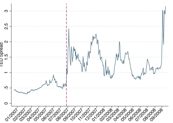
Significant strains of this nature in the inter-bank market suddenly appeared in mid-2007 amid the ongoing deterioration of the U.S. real estate market. Prior to this period, inter-bank markets were relatively calm. Nonetheless, the spread between the LIBOR and Treasury bill rates, as well as other measures of inter-bank market stress,
increased dramatically on August 9th, 2007 (Taylor and Williams (2009); Brunner-meier (2009)).8 Figure 1 highlights this dramatic increase. Amid concerns about banks’ ability to obtain liquidity via inter-bank markets, policymakers took several steps to encourage borrowing through the discount window. The Federal Reserve lowered the interest rate, expanded acceptable collateral, and increased the maturity of discount window loans (Brunnermeier (2009)). The lack of a major response to these changes led the Federal Reserve to consider a novel approach to providing access to short-term loans: establishing auctions for short-term liquidity.
1.2.1 Term Auction Facility
The Term Auction Facility provided short-term funding to banks through sealed-bid, uniform price auctions. The auctions primarily granted 28- or 84-day loans to banks with access to the discount window’s primary credit program.9 It was first announced on December 12th, 2007. The first auction occurred on December 17th, 2007. A total of 60 auctions were conducted. The last auction was held on March 8th, 2010, with this auction’s loans maturing on April 8th, 2010. The Term Auction Facility provided over $3.8 trillion in loans, with over half of the funds going to foreign banks (e.g., see Benmelech (2012)). Following the first auction for $20 billion, auction sizes increased up to $150 billion in October 2010.
The presence of binding capacity constraints in many of these auctions underlies my empirical design. Figure 2 illustrates these constraints. The blue line plots the total value of loans requested beyond the auction capacity. There was over $40 billion in unmet loan requests, for example, in the first auction due to this capacity constraint. Over the next several auctions, the capacity initially increased to $30
8Several explanations for this large increase in inter-bank spreads have been proposed, including
both an increase in counter-party risk and liquidity premiums (Taylor and Williams (2009)).
9Section 1.3.1 discusses the equilibrium bidding strategy in these auctions and highlights its
relevance for my empirical design. For more information about the Term Auction Facility generally, see https://www.federalreserve.gov/monetarypolicy/taf.htm
billion and then to $50 billion. Unmet loan requests remained high at around $31 billion, on average, during the first ten auctions. The capacity was further increased following this period to $75 billion and unmet loan requests in the subsequent ten auctions decreased slightly to around $18 billion. Binding capacity constraints were present in the first 23 auctions, with a total of over $600 billion in unmet loan requests. My sample consists of the 21 oversubscribed auctions that granted either 28- or 35-day maturity loans. Table 1 summarizes these auctions. The average over-subscribed auction had 74 bidders and slightly more than 45 bidders that received funding. The average auction granted $53 billion in loans with more than $27 billion in unmet loan requests. These 21 auctions granted 959 loans, with an average size of over $1.1 billion. There was also considerable heterogeneity in the amount of funding requested: the largest loan was for $7.5 billion and the smallest for slightly more than $1 million. The median loan size was $500 million.
Table 2 summarizes the commercial banks that bid in any of these auctions. It measures characteristics in 2007Q3, which is the quarter prior to the establishment of the Term Auction Facility. The average bidder had approximately $67 billion in assets. There was substantial heterogeneity in size: the largest bank had almost $2 trillion in assets and the smallest had only $100 million. The median bank had almost $10 billion in assets. The average bank also held three percent of its assets in cash, six percent in mortgage-backed securities, and 31 percent of its assets were loans secured by real estate. As others have highlighted, e.g. Benmelech (2012), foreign banks played an important role in this setting. Approximately, 39 percent of commercial bank bidders in the oversubscribed auctions were foreign.
A typical auction proceeded as follows. The Federal Reserve would initially de-termine the quantity of funds to provide through the auction and then announce this figure publicly along with the auction parameters. Banks could submit up to two bids in the auction, with each bid consisting of two components: an interest rate and
a loan amount.10 The interest rate must be at least the overnight indexed swap rate. The loan amount requested needed to exceed $10 million initially, but this amount decreased to $5 million in February of 2008 (Armantier and Sporn (2015)). Banks could borrow up to ten percent of the auction capacity.
Once bidding was completed, the allocation of loans was based primarily on the interest rate component of banks’ bids. Bids with the highest interest rate were initially accepted, with the Federal Reserve then accepting bids with lower interest rates until the auction capacity was, if at all, exhausted. Bids above the market-clearing interest rate, i.e. the stop-out rate, were granted the entire loan amount requested. Bids placed below this rate were not granted a loan. All banks paid the same interest rate, namely the market-clearing rate. If a bank failed to receive funding through the auction, it had three main options: seek funding elsewhere, bid in future auctions, or borrow through the discount window.
1.2.2 The Discount Window
The discount window is the traditional tool used by the Federal Reserve to sup-ply liquidity to banks facing funding problems.11 It operates under three different facilities: the primary, secondary, and seasonal credit programs. The discount win-dow’s broad objective is liquidity provision, but each program caters to a different set of banks. The primary credit program helps relieve liquidity strains by providing short-term credit to healthy banks, but it also complements monetary policy imple-mentation by providing a ceiling on the actual federal funds rate. The secondary credit program is for less healthy banks. It provides loans at higher rates and with more restrictions than the primary credit program. The seasonal credit program
sup-10Bank holding companies could submit more bids by virtue of owning multiple banks that were
individually eligible to place bids.
11This section draws from the Federal Reserve’s discount window website:
plies liquidity to smaller banks that are exposed to significant seasonal fluctuations. Nonetheless, the remaining discussion highlights the primary credit program as it accounts for most discount window borrowing and would be the main substitute for Term Auction Facility loans.
Discount window eligibility is based on several considerations. The primary de-terminant of eligibility is maintaining reserves at the Federal Reserve. This applies to foreign, as well as, domestic banks. It also applies to other institutions that hold re-serves at the Federal Reserve despite not being legally required to do so, e.g. bankers’ banks and corporate credit unions. Eligibility to borrow, broadly speaking, does not immediately imply access to the primary credit program. Banks must also be in good financial condition to borrow through the primary credit program. Good financial condition is typically defined by a CAMELS rating of one, two, or three but other supervisory information may also influence this determination.12
Banks must pledge collateral to secure any discount window loans. A variety of assets are accepted by the Federal Reserve. Some common assets used as collateral include U.S. Treasury obligations, commercial and residential loans, and corporate bonds, among others. The lendable value of any given collateral is determined by the prevailing margins set by the Federal Reserve, which vary across asset types, maturity, and other factors. The interest rate on discount window loans is determined, at a minimum, bi-weekly by each Federal Reserve bank and is applicable to banks located in each respective district. In practice, however, the rates are essentially the same across districts.13 Prior to the crisis, the primary credit rate was 100 basis points
12CAMELS refers to the different elements of banks’ financial condition that are assessed: capital
adequacy, asset quality, management, earnings, and liquidity (Lopez (1999)). Other information may indicate that a bank with a CAMELS rating of one, two, or three is not in good financial condition and, therefore, is not eligible for discount window loans. A bank with a CAMELS rating of four, which would normally indicate that the bank was not in good financial condition, can also be eligible to borrow at the discount window provided other data indicates it is healthy enough.
13The only real difference across districts is when the rate is adopted. The various Federal Reserve
districts have historically adopted the same rate, with some minor differences in the date at which the new rate commences. The differences typically manifest as one district adopting the new rate a
above the federal funds target rate.
The primary credit program provides credit with limited oversight. Primary credit program loans are, for example, granted on a no questions asked basis to eligible banks. There are also virtually no restrictions on how the funds are used. This con-trasts with the secondary credit program, which requires prospective borrowers to detail the purpose for their borrowing. The secondary credit program also prohibits borrowers from using the funds to expand their asset base. The limited administra-tive oversight and restrictions are designed to make discount borrowing through the primary credit program attractive to banks.
1.2.2.1 Replicating Term Auction Facility Loans at the Discount Window The discount window provides, in effect, a way for banks to sometimes replicate funding that they might otherwise seek through the Term Auction Facility. In my sample of auctions for 28- or 35-day loans, a bank whose bid failed could effectively replicate the same loan they sought but did not receive through the Term Auction Facility.14 A bank that failed to receive an 84-day loan through the Term Auction Facility, however, would only have a limited ability to replicate that funding structure at the discount window.
The following example illustrates this comparability. Consider a bank that bid for a loan through the auction held on August 25th, 2008. This auction provided $75 billion in 28-day maturity loans. Suppose this bank sought a $1 billion loan at an interest rate of 2.379%. The following day, on August 26th, the bank would have learned that its loan request was not accepted. Had the bank received this funding, the loan would have dispersed on August 28th and matured on September 25th. Despite its failed loan request, this bank could have requested a discount window loan for $1 day before another district.
14For the one 35-day auction in my sample, this is not exactly the case. The difference in maturities
billion on August 28th. This loan would have provided funding until September 25th, thereby producing an identical funding structure to the loan it requested, but failed to receive, through the Term Auction Facility.15 Common eligibility across these two programs implies that this option is available to all banks seeking funding through the Term Auction Facility.
The desirability of switching to the discount window naturally depends on the characteristics of discount window relative to Term Auction Facility loans. Nonethe-less, these borrowing sources share many similarities as the Term Auction Facility was designed to be an alternative to the discount window. In terms of eligibility, public disclosure, collateral requirements/haircuts, and loan terms, the two funding sources are essentially the same. While the maximum loan amount, frequency of bor-rowing opportunities, loan settlement period, and the ability to prepay differed, the discount window is better in the sense that it provides banks with more flexibility. Additionally, in the above example, the bank would have reduced interest expenses by borrowing at the discount window instead as the stop-out rate was higher than the discount window rate.16
Despite an ability to replicate Term Auction Facility loans, banks may be reluctant to use the discount window to resolve funding problems. This possibility, referred to as the stigma problem, stems from banks’ concern that their borrowing from the Federal Reserve, should it become publicly known, might send a negative signal about its health (Armantier et al. (2015)).17 There is a variety of anecdotal evidence regarding
15In two oversubscribed auctions, namely those for 84-day maturity loans, a bank cannot fully
replicate a Term Auction Facility loan at the discount window. This is due to the maturity of discount window loans being only for up to 30-days. However, my main results use only the over-subscribed auctions for 28-day or 35-day maturity loans, where banks can basically replicate the funding structure at the discount window.
16Prior to the crisis, however, a bank would not have been able to replicate the Term Auction
Facility funding structure in this manner as discount window loans were granted on an overnight basis. The overnight maturity had already been extended up to 30 days prior to the establishment of the Term Auction Facility.
17Ennis and Weinberg (2013) provide a formal model of stigma in the context of the inter-bank
the existence of stigma. Mishkin (2008), for example, notes that stigma “may largely account for the extent to which discount window borrowing has generally remained at moderate levels in recent months.” Bernanke (2009a) also highlights that “banks’ concern was that their recourse to the discount window, if it became known, might lead market participants to infer weakness.”
While discount window borrowers are not disclosed by policy, the concern is that extremely large consequences could result from the market learning of a bank’s re-liance on government support. Northern Rock, which had short-term funding prob-lems building in mid-2007, provides a good example of the concern that banks are thought to have in mind. Following failed attempts by regulators to find a buyer for Northern Rock, the BBC announced on September 13th that the bank had sought government support. The following day, the Bank of England indicated its intention to provide emergency liquidity, with a severe bank run by Northern Rock’s retail depositors immediately following (Shin (2009); Bernanke (2015)).18
Aside from the media, there are other channels through which discount window borrowers might be identified. For example, large banks may be identified from weekly aggregate data published by the Federal Reserve or, additionally, through their participation (or lack thereof) in the inter-bank market (Armantier et al. (2015)). As I obtained the identities of all Term Auction Facility bidders through a Freedom of Information Act request, this is also a possible identification channel that banks could be concerned about.19
Despite a long-standing concern over stigma, direct empirical evidence has long proved difficult to establish. Some early papers provide evidence that banks appeared
18While this example highlights a borrower from the Bank of England, it illustrates the disclosure
risk underlying stigma.
19In particular, I was able to obtain data on the identities of all banks that placed bids through the
Term Auction Facility, even those that never received funding. This includes some banks that are not found in what arenow publicly available disclosures of the Federal Reserve’s borrowers during the financial crisis.
willing to pay more to borrow in inter-bank markets when central bank funding was available at below-market rates (Furfine (2001, 2003)). While these borrowing patterns could suggest that stigma is real, some believe that the underlying data itself is problematic. Armantier and Copeland (2015), for example, show that the underlying algorithm that is used to identify loan transactions in the Federal Reserve’s Fedwire database produces errors at an alarmingly high rate. Such borrowing patterns may also reflect outdated features of the discount window - e.g., a requirement that banks exhaust all private funding sources.20 While there is good evidence of stigma during the Great Depression, e.g. see Anbil (2015), the discount window is now quite different.
Nonetheless, policymakers were concerned over stigma in the early stages of the 2007-09 financial crisis. To offset stigma’s potential impact, discount window policy was changed in several ways to encourage banks to borrow from the Federal Reserve. The spread on discount window loans, for example, was lowered on August 17th, 2007 from 100 to 50 basis points above the federal funds target rate. The maturity of discount window loans was also extended up to 30 days (Duke (2010); Armantier et al. (2015)). Despite these changes, discount window borrowing remained essentially unchanged.21 On December 12th, 2007, the Federal Reserve introduced the Term Auction Facility as an alternative to the discount window, whose primary goal was to reduce the stigma and, therefore, to improve the Federal Reserve’s ability to inject liquidity into the banking system (Bernanke (2009a); Duke (2010)).
The Term Auction Facility’s early popularity suggests that it reduced stigma. There are several explanations as to why Term Auction loans might have less stigma.
20For example, banks may appear to pay more in the private market because they are not allowed
to actually borrow at the discount window. For the most part, the discount window as it is described in this section has been in place since 2003.
21It should be noted, however, that low levels of discount window borrowing at this time could
also be explained by other liquidity available to banks through the Federal Home Loan Bank System (FHLB). Ashcraft, Bech, and Frame (2010) highlight that FHLB advances increased by $235 billion in the second quarter of 2007 to over $800 billion in total.
First, by capping how much any bank can borrow, the Federal Reserve ensures that funds are better distributed across banks. More borrowers overall provide better anonymity to any given borrower. Second, the three-day delay between auction results and loan dispersement ensures that borrowers do not have “acute funding needs on a particular day” (Bernanke (2009a)). Additionally, the auction format may serve a signaling role that the discount window cannot (La’O (2014)). Following the financial crisis, Armantier et al. (2015) provided direct evidence that the Term Auction Facility had less stigma than loans through the discount window.22
1.3 Data & Empirical Design
I employ data on bids placed for funding through the Term Auction Facility. I obtained this data by personally submitting a Freedom of Information Act (FOIA) request to the Federal Reserve. The data cover all sixty auctions and contain the identity of each bidder and the rank of each bid within the auction. While the underlying bids consist of an interest rate and quantity combination, the full bid information is protected by confidentiality and I, therefore, work with the limited sample that only contains bid ranks. I manually merge each bidder by name to its regulatory identification number with the Federal Reserve (i.e., its RSSD ID).23
The raw bidding data does not indicate which bids were ultimately accepted. To determine this, I also obtained the rank of the last bid accepted through a separate FOIA request. I then merge the bids to loan-level data on all Term Auction Facility loans. While this loan-level data was confidential at the time of my sample, it is now distributed through the Federal Reserve’s website. To measure bank performance and other characteristics, I merge the bidding data to bank balance sheet data from the
22Although they provide convincing evidence of stigma, they do not explore the broader
conse-quences of stigma on bank lending.
23In a few cases, I could not match the bidder name to a unique RSSD, owing to a general bank
name. I excluded these borrowers from the analysis. The specific banks include: City National Bank, Colonial Bank, and Guaranty Bank.
Federal Reserve’s Call & Income report.
Bidders do not necessarily correspond to the top-level of a bank holding company. I thus measure bank outcomes at the holding company level by using the parents RSSD ID to aggregate across banks. I reduce the influence of outliers by winsorizing my outcome variables at the 1st and 99th percentiles. Overall, observations in my dataset vary at the bid-level and are measured at the end of the quarter during which the auction was held. All pre-determined bank characteristics are measured in 2007Q3, which is the quarter prior to the establishment of the Term Auction Facility. As foreign banks do not report complete data, I only examine impacts for U.S. banks.24
1.3.1 Econometric Framework
My empirical design utilizes under-capacity in the early stages of the Term Auction Facility to isolate exogenous variation in short-term loans from the Federal Reserve. To evaluate the effect of this funding on bank lending, a simple approach would compare loan growth for banks that were granted loans relative to those whose bid failed owing to the auction’s capacity constraint. While intuitive, this approach will confound the effect of Term Auction loans with other unobserved variables that also influence bank lending. Potential confounding variables should, however, become irrelevant as one focuses the comparison on banks that were close to not receiving funding, but whose bid was accepted, to those banks that were close to receiving funding, but whose bid failed.
With this intuition in mind, I use variation arising from bids placed around the market clearing interest rate in each auction. A bid marginally above the market-clearing interest rate, i.e. the stop-out rate, was granted a loan in that auction, but
24In an extreme case, if foreign banks used the funding to expand lending outside of the U.S.,
then the lack of complete data would artificially create a bias towards a treatment effect of zero. Shin (2011) highlights the general view that U.S. branches of foreign banks are used to obtain dollar liquidity that is ultimately distributed to the parents’ home office abroad.
a bid marginally below this rate was not. Comparing the raw difference in average outcomes on either side of the stop-out rate facilitates a comparison of otherwise sim-ilar banks, but it is likely to significantly under-estimate the Term Auction Facility’s impact. This stems from the implicit assumption made by such a comparison: every bank whose bid fell below the stop-out rate is completely unaffected by the Term Auction Facility.
Banks can, nonetheless, pursue Term Auction Facility funding in future auctions. With auctions occurring bi-weekly, it seems likely that many banks whose bid failed could access funding through future auctions. Section 1.3.1.1 shows this is empirically relevant, with many marginal losers in a given auction ultimately obtaining funding through subsequent auctions. Thus, failure in a given auction does not imply a lack of treatment over longer time horizons, e.g. at the quarterly-level. To isolate the full treatment effect, the difference in average outcomes on either side of the stop-out rate must be scaled by the difference in the probability of obtaining Term Auction Facility loans in future auctions (Lee and Lemieux (2010); Hahn, Todd, Van der Klaauw (2001)).
Consistent with these realities, I estimate the impact of the Term Auction Facility using a fuzzy regression discontinuity design. My empirical specification is given by: yb,t=↵1+ 1QT AFb,t+h(Rankb,t) + t+✏b,t, (1) where b and t denote a specific bank and auction, respectively. yb,t denotes an out-come variable of bank b for the quarter during which auction t is held, QT AFb,t is an indicator variable that equals one if bankb receives a Term Auction Facility loan at any point within the same quarter but following the reference auction t, inclusive, Rankb,t is the bid rank of bank b’s highest bid relative to the stop-out rate in auc-tion t, t are auction fixed effects, g(·) are polynomials functions of the bid rank,
and ✏b,t is an error term. The polynomial controls, namely g(), are fully interacted with QT AFb,t implying that this specification allows the relationship between the assignment variable and yb,t to vary on either side of the stop-out rate.
My outcome variable, namelyyb,t, is growth in outstanding loan commitments. It is measured at the end of the quarter during which the auction was held. The data can therefore contain multiple observations with the same end-of-quarter outcome value arising from two distinct sources: participation in multiple auctions within the same quarter or a bank placing more than one bid in a particular auction. Using a single outcome more than once in a regression discontinuity design is consistent with other papers in the literature (e.g., see Pop-Eleches and Urquiola (2013)). I cluster my standard errors at the bidder-level to account for the correlation this induces across auctions within the same quarter for any given bidder.
My results are based on variation in Term Auction Facility borrowing induced by banks’ highest bid being placed immediately around the stop-out rate. These bids induce most of the variation in borrowing. In effect, considering only banks’ highest bid around the stop-out rate makes the designrelatively more akin to a sharp regression discontinuity design and, therefore, facilitates a visual assessment of the treatment effect using the (unscaled) difference in means at the stop-out rate.25 It also focuses the analysis on the most valuable liquidity for any given borrower.
I make two specific decisions due to the limited number of auctions to implement this research design. First, the assignment variable that I use, namely Rankb,t, is a modified version of the underlying bid rank in each auction. Specifically, in a given auction Rankb,t = +1 (-1) when bank b’s highest bid in auction t is first among other first bids in that auction to fall above (below) the stop-out rate. Other values
25There is a simple explanation as to why the variation in borrowing is “more sharp” for banks’
highest bid around the stop-out rate. When a bank’s second highest bid falls immediately below the stop-out rate, for example, it can easily obtain funding in the next auction by placing a bid that is a linear combination of its previous two bids in the prior auction.
of Rankb,t are defined similarly. Re-ranking bids in this manner is a choice driven by two interconnected issues: the small sample size of oversubscribed auctions and incomplete data for a major segment of bidders, namely foreign banks.
To illustrate the main underlying issue, Figure A.1 plots the percent of bids placed by foreign banks by the raw bid rank within each auction. It illustrates that approx-imately 40 percent of bids around the stop-out rate were placed by foreign banks. While consistent with foreign banks’ auction participation in general, the variability will be highly influenced by the sample sizes in the two ranks immediately on either side of the stop-out rate. As foreign banks do not report complete balance sheet data, their inclusion in the analysis can be problematic. Excluding these banks, how-ever, reduces the effective sample size in the ranks immediately on either side of the stop-out rate by nearly 50 percent. The re-ranking ensures that there are no “empty” ranks owing to the necessary exclusion of foreign banks and, therefore, enhances the precision of the average loan growth on either side of the stop-out rate.
Second, I specifically “break” apart an indicator for ever borrowing from the Term Auction Facility during the quarter into two parts: borrowing prior to the reference auctiontand, separately, future borrowing following the reference auctiont. In effect, my main endogenous variable is always “forward-looking” by only measuring borrow-ing in that auction and any future auction within the same quarter. This approach acknowledges that all of the variation in quarterly borrowing induced by capacity constraints operates through future borrowing (relative to the reference auction t) within the same quarter. This latter point follows because at the time auction t oc-curs, past borrowing within the same quarter is a pre-determined variable and, hence, is balanced at the stop-out rate. A forward-looking measure maximizes the power of the first-stage in my empirical design.26 In effect, such a measure uses the limited
26To highlight the empirical relevance of this, the reader is referred to Figure A.2 and Table A.1.
Figure A.2 shows that discontinuous changes in total borrowing within the quarter are visually evident. However, Table A.1 shows that, despite being economic large, under one specification the
data more efficiently by acknowledging how the treatment dynamics are (and are not) influenced by any given auction.
Overall, my primary interest is to uncover the value of 1. This coefficient
an-swers the main research question: did this auction-based liquidity matter? When yb,tmeasures loan growth, a positive value of 1 indicates that this funding increased
bank lending. The main requirement to identifying 1 is that only a discrete change
in treatment arises at the stop-out rate. As banks can bid for funding in future auc-tions, only the probability of borrowing from the Term Auction Facility is likely to vary discretely as one moves from one side of the stop-out rate to the other. I there-fore estimate 1 by using an indicator of having a bid placed above the stop-out rate
in a given auction as an instrument for future borrowing through the Term Auction Facility in the same quarter.
More formally, let T AFb,t be an indicator variable that equals one when bank b’s highest bid in auction t is above the stop-out rate. Equation 1 is then estimated using two-stage least squares (2SLS) withT AFb,tused as an instrumental variable for QT AFb,t. The first stage of this 2SLS estimation is given by:
QT AFb,t=↵0+ 0T AFb,t+g(Rankb,t) + t+ b,t, (2) where 0 captures the difference in the probability of ever borrowing by the end of
the quarter at the stop-out rate. A necessary condition for a valid fuzzy regression discontinuity design is that 0 6= 0, which indicates that the instrument is relevant
and, more specifically, that it isolates a source of exogenous variation in the otherwise endogenous variable QT AFb,t. The inclusion of the polynomial function of bid rank, namely g(·), and the auction fixed effects ensures that the variation used to identify 1 is based solely off of banks that bid close to, but on either side of, the stop-out
rate in the same auction.
This empirical strategy isolates variation in access to funding for banks that, arguably, have the smallest valuation. This is a natural consequence of bid rank as an assignment variable, which roughly captures bidders’ valuations. The effects, therefore, likely understate the Term Auction Facility’s impact for banks whose bid was well above the stop-out rate. This is advantageous because extrapolating to other banks above the stop-out rate provides conservative estimates for these banks.
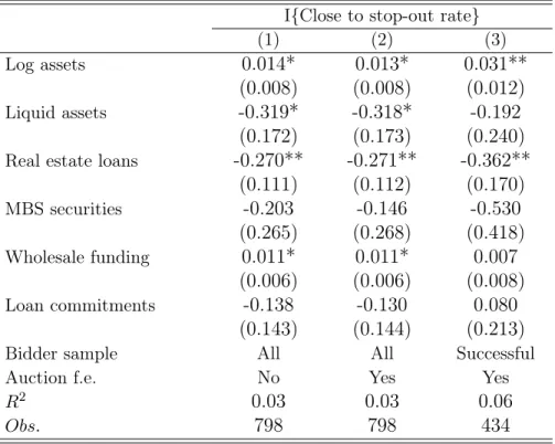
Table 3 provides more on this point. It correlates the characteristics associated with being close to the stop-out rate.27 Columns 1 and 2 compare close bidders to non-close bidders across all auctions and within the same auction, respectively. Both columns show that being close to the stop-out rate is associated with lower exposure to real estate. External validity, however, relates more to whether banks at the stop-out rate are comparable to other banks that were well above the stop-out rate. Consequently, Column 3 presents a similar result that conditions on receiving some funding in the auction. It also shows that banks close to the stop-out rate were larger than those above it. As size correlates with access to other funding sources, both relationships are consistent with effects at the stop-out rate underestimating effects for banks above this rate.
Second, the variation inQT AFb,tarises from the impact of having a bidmarginally fail in a given auction on the likelihood of ever being successful in obtaining Term Auction Facility loans in future auctions. To see this, note that while a bid placed above the stop-out in a given auction ensures thatQT AFb,tequals one, not all banks with failed bids, as noted earlier, will have QT AFb,t equal to zero. The variation in QT AFb,t arising from the instrument is thus due to banks that are never successful in obtaining Term Auction Facility loans because their bid in a given auction marginally failed.
It is useful to highlight why marginally failing identifies a discrete change in bor-rowing at a longer time horizon. Initially, note that there are two reasons why a bank could be successful in future auctions despite having their initial bid fail. First, the bank might have initially bid below its valuation. Such bid shading is indeed a fea-ture of this auction setting - e.g., see Wilson (1979), Kastl (2011), and Ausubel et al. (2014). A bank could overcome a previously unsuccessful bid by reducing the degree to which it shades it bid. Second, a bank’s valuation for funding may be increasing (at least relative to other bidders) over time. The bank’s bid would then eventually exceed the stop-out rate in future auctions. These observations suggest that marginal losers would be especially able to overcome a failed bid as they were already bidding close to the stop-out rate.
A simple example highlights why marginally failing could nonetheless capture a discrete change in future borrowing. For simplicity, assume that there is no bid shading nor any growth in banks’ valuations. If the supply of short-term funds remains constant through time, then a failed bid in a particular auction will perfectly predict being unsuccessful in future auctions. This occurs because a bank with a valuation marginally below the market clearing rate has no room to adjust its bid since it already equals its valuation. The amount of variation in borrowing that is identified from this empirical design is, thus, an empirical matter. The next section highlights the variation in treatment at the stop-out rate.
1.3.1.1. Term Auction Facility Borrowing at the Stop-Out Rate
I begin by highlighting marginal losers’ propensity to pursue funding in future auc-tions. Table 4 presents the bidding data across U.S. banks. It indicates that 85 percent of banks that fell one below the stop-out rate bid in the next auction. Ap-proximately 90.5, 57.1 and 70 percent of banks that fell two, three, and four below the stop-out rate also bid in the next auction. Repeated bidding is clearly important in
this environment. Nonetheless, it does not immediately follow that banks whose bid failed in a given auction are ultimately successful at actually obtaining Term Auction Facility loans in future auctions.
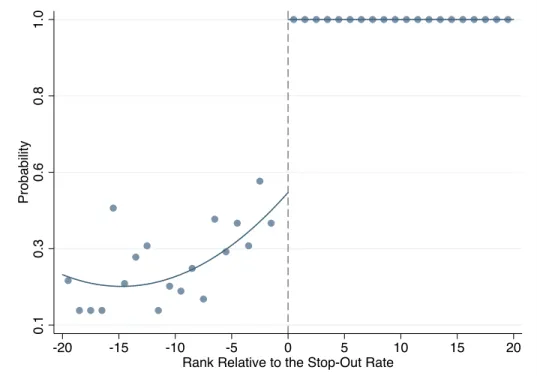
Figure 3 evaluates this possibility. It plots the relationship between the proba-bility of receiving a loan request in a given auction and banks’ bid rank. Given the institutional setting, banks with bids above the stop-out rate receive their loan re-quest, which is indicated with a positive bid rank, whereas those below the stop-out rate do not. This is visually represented as a jump in the probability of receiving a loan in the auction moving from zero on the left of the stop-out rate to one on the other side. This panel plots the instrument, namelyT AFb,t, underlying my fuzzy regression discontinuity design.
Figure 4 plots the relationship between the probability of receiving a Term Auction Facility loan by the end of the quarter and a banks’ bid rank. This chart expands on Figure 3 by incorporating a broader time horizon. The dependent variable in this chart is the main endogenous treatment variable, namely QT AFb,t from Section 1.3.1. It is measured relative to a reference auction. Bid rank is thus the rank within the reference auction and the dependent variable accounts for access to funding in the reference auction or through any subsequent auction within the same quarter. As noted earlier, all banks that receive a loan in a given auction, by definition, also receive a loan within the same quarter as that auction, which is why the charts in Figures 3 and 4 are identical above the stop-out rate. The relevant issue is whether banks below the stop-out rate ultimately obtain Term Auction Facility loans in future auctions.
Figure 4 illustrates that banks are partially successful in this regard. It is apparent that a considerable percent of banks with failed bids obtain funding in future auctions as shown on the left side of the stop-out rate. The chart illustrates that, conditional on being below the stop-out rate, there is a positive relationship between interest
rate bid and the probability of borrowing by the end of the quarter. About 15 percent of banks, for example, with a bid that fell 20 ranks below the stop-out rate obtain funding at some point within the quarter. This figure increases to around 50 percent for banks whose bid was immediately below the stop-out rate. This jump in the probability of borrowing is the exogenous variation in access to Term Auction Facility loans that underlies my main empirical results.28
Table 5 provides the empirical results that correspond to this visual evidence. It presents the results using the optimal bandwidth of +/- 7 bids around the stop-out rate and, additionally, using all of the data, but more flexible controls for bid rank.29 Panel A of Table 5 indicates that approximately 50 percent of marginal losers obtain Term Auction Facility loans within the quarter. This is indicated by a discontinuity of approximately 50 percentage points at the stop-out rate, which is economically large and statistically significant. The magnitude of the discontinuity decreases only slightly when I do not restrict to +/- 7 bids, but it is still large at around 47 percentage points and statistically significant. Banks are clearly able to partially overcome failing by pursuing funding in future auctions.
1.3.1.2. Balance of Baseline Covariates at the Stop-Out Rate
A valid regression discontinuity design hinges on the continuity of baseline covariates at the stop-out rate. Table 6 provides estimates of the average pre-existing differences at the stop-out rate. It examines six characteristics measured as of 2007Q3: the natural log of bank size, total loans (relative to assets), loans secured by real estate (relative to assets), mortgage-backed securities holdings (relative to assets), deposits
28While Figure 3 suggests that the variation in treatment is along the extensive margin, my
results are actually capturing intensive margin changes. Many of these banks had borrowed in previous auctions within the quarter. Although the extent to which they have done so is balanced at the stop-out rate. This balance is due to outcomes in past auction auctions, even those within the same quarter, in effect being pre-determined variables.
(relative to liabilities), and wholesale funding (relative to assets). The results indicate that there are no significant discontinuities in any of these variables. Figure 5 plots these characteristics against the banks’ bid rank. The x-axis measures the distance of each bid from the stop-out rate, with a positive value indicating the bid was accepted and a negative value indicating the bid failed, i.e. the borrower was not granted a loan. A circle indicates the average value within that bid rank and vertical bars plot 95-percent confidence intervals. Visually, there are no significant discontinuities at the stop-out rate.
Banks may nonetheless differ along unobservable dimensions at the stop-out rate. Marginal winners did, for example, place a higher bid than marginal losers. This might suggest one unobserved difference: a higher valuation for emergency funding. Nonetheless, there is unlikely to even be a one-to-one relationship between banks’ valuations and their bids near the market-clearing rate. When banks are restricted from submitting continuous bid functions, as they are in this context, bids may be placed above marginal values when there is a positive probability of the bid falling below the market-clearing interest rate (Kastl (2011)). This indicates that one cannot infer from marginally winning that a bank must have a valuation that is weakly larger than the marginal losers. Even small differences in marginal valuations is tolerable within a regression discontinuity design, provided there is not a discrete change at the stop-out rate.30
Banks could also strategically sort in a way that generates differences in other un-observables at the stop-out rate. While one cannot test for such discontinuities, there are two reasons to doubt they are present. First, the stop-out rate is unknown at the time of the auction. Uncertainty in the level of demand for Term Auction Facil-ity loans alone implies that only the distribution of the stop-out rate is (potentially)
30I did place a separate FOIA request to obtain information on differences in the interest rate bid
known ex ante. Second, even with limited uncertainty, extremely small differences in bids can determine when the auction’s capacity is exhausted. Bids can be sub-mitted with interest rates specified up to three decimal places, implying that the difference between marginally winning and losing can be determined by arbitrarily small differences in bids.
1.4 Results
I evaluate the impact of the Term Auction Facility. I focus on banks’ growth in outstanding loan commitments. In the seminal model of Kashyap, Rajan, and Stein (2002), banks provide liquidity to borrowers via loan commitments, which are con-tractual agreements to provide funding. To effectively do this, banks must hold liquid assets to help fund unpredictable drawdowns. Liquidity pressures can therefore dam-age banks’ ability to commit new funding to borrowers.
Loan commitments are an important component of financial intermediation. The Federal Reserve’s Survey of Terms of Business Lending indicates, for example, that approximately 80 percent of commercial loans in general, 85 percent of those granted by U.S. banks, and 87 percent granted by large U.S. banks are made under commit-ment as of 2007Q3.31
I specifically focus on outstanding loan commitment growth. This outcome vari-able thus measures the “unused” component of the commitment. Captured in this manner, outstanding commitments increase either when banks grant more loans or because borrowers reduce drawdowns on pre-existing credit lines. Both outcomes are possible responses to Term Auction Facility funding. The former possibility is simple: banks may intermediate more if they borrower more. The latter could arise if banks sought Term Auction Facility funding to compensate for a borrower-based run on
pre-existing credit lines. Ivashina and Scharfstein (2010) show that borrowers ran on lines of credit during the crisis.
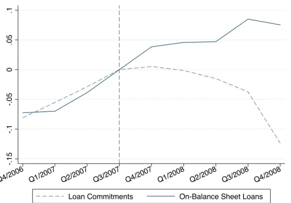
Focusing on this variable is valuable from two perspectives. First, outstanding commitments were quickly declining in the early stages of the crisis. Figure 6 high-lights this decline. It plots the evolution of aggregate outstanding commitments and on balance sheet loans. Each line is the natural log of the level, with values normal-ized as of 2007Q3. As a result, the value at each point in time captures the percent difference between the level at that point in time relative to 2007Q3. The dashed line is for outstanding commitments, whereas the solid line is for on-balance sheet loans. While both variables were increasing leading up to the crisis, it shows that by 2008Q4 outstanding commitments declined by over 10 percent below its 2007Q3.
Second, this variable yields more statistical power. There is more power as the outcome responds in the same way to the lending and credit line run-based chan-nels. Even if one did not know which channel was at work, an impact on outstanding commitment growth is nonetheless economically interesting. Consider my null hy-pothesis: auction-based liquidity via the Term Auction Facility did not matter. Also note that my empirical design compares marginal winners relative to banks that can replicate the same funding through the discount window. The results should then capture banks’ outstanding commitment growth relative to that growth had only dis-count window funding been in place. Nonetheless, I distinguish between these two alternative explanations through additional results.
I initially highlight the Term Auction Facility’s impact in several ways. I first con-firm the absence of pre-existing differences in outstanding loan commitment growth at the stop-out rate. A discontinuous change, if it were to exist, would cast doubt on my empirical design by suggesting that within-sample differences in my outcome variable arise for reasons other than the Term Auction Facility. Figure 7 plots outstanding commitment growth in 2007Q3, which is the quarter before the establishment of the
Term Auction Facility. The x-axis measures banks’ bid rank relative to the stop-out rate. Positive and negative values indicate that a bid fell above and below the stop-out rate, respectively. Each blue dot displays the average outstanding loan commitment growth within each rank. The vertical lines denote 95-percent confidence intervals. The grey lines are third-order polynomials on either side of the stop-out rate. This chart illustrates the absence of any pre-existing discontinuity.
Panel A of Table 7 provides the statistical evidence corresponding to Figure 7. It presents the evidence in two main ways. Columns 1 and 2 provide the results using only data within the optimal bandwidth, i.e. +/- 7 bid ranks around the stop-out rate, and control for banks’ bid rank using linear and quadratic polynomials. Columns 3 and 4 provide the results when I do not restrict the sample to the optimal bandwidth, henceforth “using all of the data”, but include more flexible controls for bid rank. Overall, these results confirm the qualitative evidence in Figure 7. The point estimates are all close to zero and insignificant. The absence of any discontinuity as of 2007Q3 contrasts with after the Term Auction Facility was established.
Figure 8 plots outstanding commitment growth against banks’ bid rank within the sample following the establisment of the Term Auction Facility. A discontinuity at the stop-out rate is evident. Panel B of Table 7 provides estimates the magnitude. It also presents the results using the optimal bandwidth and, separately, using all the data. The point estimates are very similar, ranging from 0.06 to 0.13, indicating that the outstanding loan commitment growth of marginal winners is at least 6% more than marginal losers. Nonetheless, the difference in average outcomes must be scaled by the change in the probability of treatment at the stop-out rate to reflect the Term Auction Facility’s full impact (Lee and Lemieux (2010); Imbens and Lemieux (2008)). Table 8 provides the fuzzy regression discontinuity design estimates of the average treatment effect of the Term Auction Facility. It uses an indicator for receiving a loan in a given auction as an instrument for ever borrowing by the end of the quarter.
Section 1.3.1 highlighted that this empirical strategy leverages marginally losing to isolate exogenous variation in Term Auction Facility borrowing at the quarterly-level. Panel A presents the 2SLS first stage, which illustrates the relationship between the endogenous treatment variable and the underlying instrument. Columns 1 and 2, which use the optimal bandwidth, and Columns 3 and 4, which use all the data, indicate a strong first stage relationship. The point estimates are statistically signifi-cant and range from 0.49 to 0.57 across specifications. They indicate that marginally losing isolates an economically relevant jump in the probability of borrowing by the end of the quarter of about 50 percentage points.
Panel B of Table 8 highlights the Term Auction Facility’s impact. It provides the estimates of 1 in Equation 1. The point estimates can be derived as the raw
difference in average loan commitment growth, e.g. in Panel B of Table 8, divided by the difference in the probability of ever borrowing from the Term Auction Facility on either side of the stop-out rate. The results are significant and economically large. They indicate that the Term Auction Facility increased outstanding loan commitment growth by over 15 percentage points. The effect is consistent with a large aggregate decline in outstanding loan commitments at this time.
With outstanding commitments measuring the “unused” component of commit-ments, an increase can arise either when banks grant more loans or because bor-rowers stop drawing down on their pre-existing lines of credit. An increase in loan commitments due to Term Auction Facility funding, therefore, could merit a different interpretation: borrowers were concerned about their lender’s health and they were, consequently, drawing down on pre-existing lines of credit to ensure their access to credit, and access to Term Auction Facility funding ultimately arrested this bank run. While such precautionary draw-downs have been documented in the literature, Term Auction Facility borrowing was confidential and so banks might have to reveal this information to their borrowers under this alternative interpretation. As