Detection of Patches of Outliers in Stochastic
Volatility Processes
Anderson C.O. Motta
Banco Ita´u-Unibanco
E-mail address: [email protected]
Luiz K. Hotta
Department of Statistics, University of Campinas
Rua S´ergio Buarque de Holanda, 651; 13083-859; Campinas, SP; Brasil
E-mail address: [email protected]
Abstract. Because the volatility of financial asset returns tends to arrive in clusters, it is quite likely that outliers appear in patches. In this case, most of the statistical tests developed to detect outliers have low power. We propose to use the posterior distribution of the size of the outlier and of the probability of the presence of an outlier at each observation to detect and estimate the outlier. This sampling algorithm is an adapted version of the algorithm proposed by Justel et al. (2001) for autoregressive time-series models. Our proposed sampling procedure is applied to a simulated sample according to the stochastic volatility, a sample of the New York Stock Exchange daily returns, and a sample of the Brazilian S˜ao Paulo Stock Exchange daily returns.
1. Introduction
The stochastic volatility (SV) model (Harvey et al. (1994), Ghysels et al. (1996)) has had great success in the study of financial time series. A large part of this success results from the ability to explain part of the heavy tails and volatility clustering. According to Kobayashi (2006) “The estimation of the stochastic volatility (SV) models with jumps has been an important topic in financial econometrics, because the excess kurtosis that cannot be explained by the simple SV model is often attributed to jumps
Key words: Patches of outliers; Stochastic volatility; Detection of outliers; Markov chain Monte Carlo.
in returns and volatility.” In other words, there are still some observations and changes that cannot be accommodated or explained by these models. This scenario is a matter of concern because empirical studies have shown that a small number of these observations can have a large effect on the model estimation and can lead to poor model specification. Therefore, it is necessary to find statistical tools to uncover these observations. The correct detection of these observations can provide valuable information about the series that is under analysis. Another feature of finance data is that the outliers come in patches because the effect of an unexpected extreme “good” or “bad” piece of news can last for more than one day. In this case, most of the statistical tests developed to detect outliers have low power. To overcome a similar problem in autoregressive processes, Justel et al. (2001) based a study on the McCulloch and Tsay (1994) Bayesian approach, and presented a procedure to detect and estimate patches of outliers in these processes. They used the posterior distributions of the size of the outlier and of the probability of the presence of an outlier at each observation to detect and estimate the outlier size. The methodology was shown to have good power for autoregressive processes. We use the same concept to detect patches of outliers in stochastic volatility processes. This procedure is applied here to simulated and empirical data sets.
There are other approaches suggested in the literature for detecting out-liers in SV models, for example, by comparing posterior Bayes odds as in Eraker et al. (2003), by an excess of skewness as in Bates (2000), and by testing a moment condition on the options prices as in Pan (2002). Another possibility is the use of the method proposed by Chib (1995), i.e., to compare the log marginal likelihoods under both models.
This article is organized as follows. Section 2 presents a brief review of the tests proposed to detect outliers in volatility models, mainly in GARCH and SV models, the SV model with additive or level outliers, and the model likelihood. Section 3 presents the adaptation of the methodology of Justel et al. (2001) to detect patches of outliers in SV model. It also presents the priors and the conditional posteriors necessary to implement the MCMC estimation procedure. Section 4 illustrates the methodology with simulated data and the study of the continuously compounded daily return of the New York Stock Exchange composite index (NYSE), which was previously analyzed by Zhang (2004) and Zhang and King (2005), and the Brazilian S˜ao Paulo Stock Exchange return index (IBOVESPA). Section 5 presents the final remarks.
2. SV models with level outliers
There is a large amount of literature on outlier tests in time series mod-els, but most of the studies are related to ARMA models. The Chen and
Liu (1993) procedure, which is one of the most used methods, is an itera-tive procedure that jointly estimates the model and the outliers to reduce the masking effect. McCulloch and Tsay (1994) presented a Bayesian ap-proach to detect outliers in autoregressive models using Gibbs sampling, and they showed that the procedure has good power in detecting isolated outliers. However, the iterative procedures can have low power when the outliers occur near each other, i.e., in patches. Patches of outliers can ap-pear in time series for many reasons. For example, Tsay et al. (2000) showed that an innovation outlier in a multivariate process could generate patches of outliers in a marginal univariate time series. To overcome this problem, Justel et al. (2001) based a study on the McCulloch and Tsay (1994) Bayesian approach and presented a procedure to detect and estimate patches of outliers in autoregressive processes.
More recently, articles have appeared in the literature that address out-liers in volatility models. Because it is easier to work with GARCH models, most of the work on volatility outliers is related to GARCH models. See, for example, van Dijk et al. (1999), Zhang (2004), Zhang and King (2005) and Hotta and Tsay (2012). In the stochastic volatility models the outliers are usually referred to as jumps. We can cite Chib et al. (2002), Liesenfeld and Richard (2003), Jacquier et al. (2004), Kobayashi (2006), Liesenfeld and Richard (2006), Omori et al. (2007) and Nakajima and Omori (2009) regarding the SV models.
The SV model with an additive or level outlier (LO) is given by the following:
yt = δtβt+e
ht
2 t (1)
ht = µ+φ(ht−1−µ) +σηηt,
where |φ| < 1 and t and ηt, t = 1,· · · , n, have independent standard
Gaussian distributions. We also use the use the following reparametrization for the SV model:
yt = δtβt+γe
ht
2 t (2)
ht = φht−1+σηηt,
whereγ = expµ/2, i.e. a positive parameter. The notationδtis an indicator
function that is equal to one whenever an LO is present at the t-th observa-tion and zero elsewhere, i.e., it has a Bernoulli distribuobserva-tion with parameter κ (denoted as δt ∼Ber(κ)). The random variable βt indicates the size of
the outlier at the t-th observation with the log normal distribution ψt= log(1 +βt)∼N(−0.5ν2, ν2),
following Andersen et al. (2002). Denote the n-dimensional vector of the returns as y = (y1,· · · , yn)0, the vector of (log) volatilities as h =
(h1,· · · , hn)0, the vector of outlier indicators asδ= (δ1,· · ·, δn)0, the vector
of outlier amplitudes asβ= (β1,· · ·, βn)0, and their transformed values as
ψ = (ψ1,· · · , ψn)0. Denote the vector of parameters asΘ= (µ, φ, σ2η, κ, ν)0.
For the sake of simplicity we will use the same name of the vector of param-eters Θ when use the parametrization µ or γ. The posterior distribution of Γ= (Θ0,h0,β0,δ0)0 is
π(Γ|y)∝p(y|Γ)p(h|β,δ,Θ)p(β,δ|Θ)p(Θ), (3) wherep(y|Γ) is the likelihood of ygivenΓ,p(h|β,δ,Θ) is the conditional density ofh,p(β,δ|Θ) is the conditional density of (β0,δ0)0, andp(Θ) is the prior of Θ. Because of the independence of β and δ we have p(β,δ|Θ) = p(β|Θ)p(δ|Θ). The same is valid for Γ when we use the parametrization
β orΨfor the size of outliers.
3. Estimation: priors and conditional posteriors
The model is estimated by the MCMC technique, which was first pro-posed by Jacquier et al. (2004) in the SV context. In this section, we present the priors and conditional posteriors necessary to implement the algorithm. In Subsection 3.4, we present the standard method to sample the probability of the presence of the LO. This approach is used in the liter-ature, for example, by Chib et al. (2002), Liesenfeld and Richard (2003), Jacquier et al. (2004), Kobayashi (2006), Liesenfeld and Richard (2006),
Omori et al. (2007) and Nakajima and Omori (2009). In Subsection
3.5, we present our contribution, where we first detect possible intervals of observations with patches of outliers, and later we show how to sam-ple in block, in each interval, the probabilities and size of outliers for each observation in the intervals.
3.1. Sampling (σ2η, φ). We follow Kim et al. (1998) and Shephard and Pitt (1997) in samplingσ2
η andφ. Observe that, conditional tohandµ, we
have a regression model. Therefore, using the inverse Gamma distribution IG(σr/2, Sσ/2) as the prior distribution ofση2, the full conditional posterior
distribution is given by the inverse Gamma distribution:
ση2|y,h, φ, µ,β,δ∼ ∼IG n+σ r 2 , Sσ+ (h1−µ)2(1−φ2) +P n−1 t=1((ht+1−µ)−φ(ht−µ))2 2 .
Following Kim et al. (1998) and Shephard and Pitt (1997), we takeσr= 5
Reparameterizing φ = 2φ∗−1 and using as prior distribution of φ∗ a beta distribution with parameters (φ(1), φ(2)), the prior ofφis given by the following: π(φ)∝ (1 +φ) 2 φ(1)−1 (1−φ) 2 φ(2)−1 , φ(1), φ(2) > 1 2, (4)
and the parameterφcan be sampled from the complete conditional density using the rejection method as follows.
Considering the prior (4), the complete conditional distribution of φ is proportional to the following:
π(φ)f(h|µ, φ, ση2,β,δ), where logf(h|µ, φ, σ2η,β,δ)∝ − (h1−µ)2(1−φ) 2σ2 η +1 2log(1−φ 2)− − Pn−1 t=1{(ht+1−µ)−φ(ht−µ)} 2 2σ2 η .
This function is concave inφfor any value ofφ(1) and φ(2). Therefore, we can sample φ using the rejection sampling algorithm. Kim et al. (1998) took the Taylor expansion of the prior with respect to the following value:
ˆ φ= Pn−1 t=1(ht+1−µ)(ht−µ) Pn−1 t=1(ht−µ)2 .
Therefore, given a proposed value φp from N( ˆφ, Vφ), where Vφ =
σ2
η{
Pn−1
t=1(ht−µ)2}−1this value is accepted with the probability exp{g(φp)−
g(φ∗(i−1))}, whereφ∗(i−1) is the sample from the previous (i-1)-th MCMC iteration, and g(φ) = logπ(φ)−(ht−µ) 2(1−φ2) 2σ2 η +1 2log(1−φ 2).
If the proposed value is rejected, then we take φ∗(i)=φ∗(i−1)
3.2. Sampling µ. Conditional toφ, σ2η andh we have a regression model. Thus, taking a diffuse prior forµ, the posterior distribution is sampled from the complete conditional distribution given by the following:
where ˆ µ=σµ2 (1−φ2) σ2 η h1+ (1−φ) σ2 η n−1 X t=1 (ht+1−φht) , and σ2µ=ση2{(n−1)(1−φ2) + (1−φ2)}−1.
3.3. Sampling the volatilities. Jacquier et al. (2004) proposed a
Bayesian approach to theSV model, exploring the structure of the model. After this seminal paper, several modifications were proposed to improve the efficiency of the simulation chain. See, for example, Shephard and Pitt (1997), Kim et al. (1998), Chib et al. (2002), and Chib et al. (2009). Kim et al. (1998) used a mixture of normal distributions and, conditioned on the mixture distribution, used the Kalman Filter to jointly sample all of the volatility vectors. They also proposed to jointly sample all of the model parameters in order to minimize the chain dependence. Chib et al. (2002) generalized the method proposed by Kim et al. (1998). They used covariates and modified the distribution of the disturbances to capture the type of effect of outliers found in empirical financial series. Zhang and King (2005) used a single-move random-walk Metropolis-Hasting algorithm.
There are some differences in the papers cited above. Motta and Hotta (2003) and Liesenfeld and Richard (2006) present a comparison of these studies. We samplehusing the simulation smoother (de Jong and Shephard , 1995; Durbin and Koopman , 2002).
3.4. Standard sampling of the probabilities and sizes of outliers.
From Section 2 we have that δt ∼ Ber(κ) and ψt = log(1 + βt) ∼
N(−0.5ν2, ν2). We consider the prior distribution of κ given by κ ∼
Beta(u0, n0) and the prior distribution of ν given by ν ∼ LN(ν0, N0),
where LN means lognormal distribution. The parameter κ can be
sam-pled directly from the posterior because we have a conjugate family. The parameterν is sampled using the acceptance-rejection Metropolis-Hasting algorithm (Tierney , 1994). The hyperparameters u0, n0, ν0 and N0 will
be given later.
The procedures for jointly estimating the model and detecting the out-liers are based on the posterior distributions. Thus, we must calculate the posterior distributions of δt and βt. The marginal posterior distributions
of the elements ofδ are given by the following: pt = p(δt= 1|y) = X δrt p(δrt|y) = X δrt Z p(δrt|y,Ψ)p(Ψ|y)dΨ ∝ X δrt Z p(y|δrt,Ψ)p(δrt)p(Ψ|y)dΨ, t= 2, . . . , n,
where the sum is over all of the 2n−1 outlier configurations, δrt denotes a configuration, and p denotes the probability density function for discrete and continuous distributions. The posterior distributions of the size of the outlier are given by the following:
p(βt|y) =
X
δrt
p(δrt|y)p(βt|y, δrt) t= 2, . . . , n.
3.5. Sampling probabilities in a block. McCulloch and Tsay (1994)
used Gibbs sampling to sample from the posterior distributions of the prob-abilities and of the size of additive outliers in autoregressive models. Justel et al. (2001) showed that the McCulloch and Tsay (1994) procedure has good power in detecting isolated outliers in autoregressive models but is inefficient in the presence of patches of outliers. To overcome this problem, Justel et al. (2001) proposed an algorithm in two stages. In the first stage, they identify a possible patch of outliers, and in the second stage, they identify the observations within the block that are affected by the outliers. The first stage uses the standard method to sample the probabilities and the size of the outliers. In the second stage, the sampling is performed in blocks in each patch. The priors for the second stage are the same as those in the first stage. The two stages are presented below, and the block sampling described in Subsection 3.5.2.
3.5.1. Procedure to detect possible patches of outliers. In this section, we consider the first stage of the Justel et al. (2001) procedure to detect patches of outliers. Initially, we must define two critical values, c1 and c2,
withc2 < c1 and d. Whilec1 is defined in step (2),c2 anddare defined in
step (3). The procedure consists of the following steps:
(1) Estimate the model, and denote the estimated probability of the presence of an outlier in the t-th observation by ˆpt. Call the
(2) The ti-th observation is suspected of being an outlier if ˆpt > c1.
LetT∗ ={t1,· · ·, tm} be the set of observations that are detected
as possible outliers in this step. Justel et al. (2001) suggested considering the total number of possible outliers to be at most equal ton/2. Thus, ifm > n/2,the we must increase c1;
(3) Consider the second critical value, c2 < c1, to test whether the
2dobservations that are nearest to each one of the m observations found in step (2) are possible outliers. An observation is included in the window test as a possible outlier if ˆpt> c2;
(4) For each value ti ∈T∗ define ki = max{0,1,· · · , d}, with yti−ki > c2, and vi = max{0,1,· · · , d}, with yti+vi > c2. The possible block of outliers related to the observationyti is given by the block (yti−ki,· · · , yti+vi). Note that, as max(ki, vi) ≤ d, the maximum length of the block is (2d+ 1);
(5) Any set of consecutive intervals with juxtaposition is concatenated in a unique block. Thus, the number of possible blocks can be less thanm, and the length of the blocks is unlimited;
(6) The total number of possible outliers is given by the number of observations covered by the blocks. If this number is larger than n/2, then the critical valuec2must be increased and/or the value of
dmust be decreased. As a third alternative,c1 should be increased;
(7) For each block of observations identified as possible outliers re-estimate the posterior probability. The next subsection shows how to estimate the probability inside the blocks. Call the estimates in this step the Adapted Gibbs Sampler estimates.
3.5.2. Posterior distribution for the block of outliers. After identifying the possible block of outliers, it is reasonable to sample simultaneously inside the blocks using Gibbs sampling. To perform this sampling, we must find the posterior distributions of a block starting, for example in thej-th ob-servation with a size of, for example, k Then, δj,k = (δj, . . . , δj+k−1)0 and
βj,k = (βj, . . . , βj+k−1)0 are the indicator and size of the outliers,
respec-tively.
The posterior distribution of Γ = (Θ0,h0,β0,δ0)0 is given by equation 3. Because we do not have a closed form for the density, we will use the MCMC to sample from the density. We will use the method presented by Kim et al. (1998). Rewrite the model as follows:
y∗t = ht+zt
ht = µ+φ(ht−1−µ) +σηηt,
where
and the distribution of zt = log2t is approximated by a mixture of
nor-mal distributions. The complete conditional distribution is given by the following:
P(δj = 1|y,h,Ψ,Θ, k, δ(j)) =
kfN(ytkβt, eht)
kfN(ytkηt, eht) + (1−k)fN(ytk0, eht)
, where δ(j) is obtained from δ by eliminating the component δj, and
fN(ytkµ, σ2) denotes the density of the normal distribution with a mean µ
and variance σ2 evaluated at yt. For the size of the outlier, we have that
ψt|y,Θ,δ,Ψ(j), ht∼N(ψj∗, b−1), where b= σ 2 η +δt2 ν2σ2 η and ψt∗= −0.5σ 2 η +δtyt bσ2 η .
We need the joint distribution of the size of of all the outliers in the block to obtain the joint samples. Denote byΓ(δ
j,k)andΓ(βj,k)the vectorΓ elim-inating the vectors δj,k and βj,k, respectively. The posterior distributions
of δj,k andβj,k, are given, respectively by:
p(δj,k|y,Γ(δ
j,k)) ∝ p(y|Γ(δj,k);δj,k)·κ
sj,k(1−κ)k−sj,kp(κ), p(βj,k|y,Γ(β
j,k)) ∝ p(y|Γ(βj,k);βj,k)·p(βj,k|ν)p(ν),
where sj,k = Pjt=+jk−1δt, and p(κ) and p(ν) are the prior distributions of
κ and p(ν), respectively, and given in Subsection 3.4. The distributions of the size of the outliers inside each block, conditional toν are independent. The first likelihood can be factored as follows:
p(y|θδ j,k;δj,k) =p(y j−1 2 |θδj,k)· ·p(yTj,k j |y j−1 2 ;θδj,k;δj,k)·p(y n Tj,k+1|y Tj,k 2 ;θδj,k), where ykj = (yj, . . . , yk)0 and Tj,k = min{n, j+k}. For the LO model (1),
the density is given by the following:
p(yTj,k j |y j−1 2 ;Γ(δj,k);δj,k)∝ min{n,j+k} Y t=j fN(yt|ht,Θkδtβt;eht)fN(ht|h(t),Θkµ+φ(ht−1−µ);ση). The likelihood p(y|Γ(β
j,k);βj,k) can be factored in a similar way. Now, we have all of the results that are necessary to apply the Gibbs sampler in
step (7), and we can sample from the posterior distribution ofδj,k andβj,k
to estimate their distributions.
In summary, the sampling procedure for (Θ0,h0,δ0,β0)0 is as follows:
• sample φ from the rejection sampling algorithm (see Subsection 3.1);
• σ2η directly from the inverted Gamma density (see Subsection 3.1);
• sampleµdirectly from the Gaussian density (see Subsection 3.2);
• sampleh by simulation smoother (see Subsection 3.3);
• The standard sampling ofδ and β is given in Subsection 3.4. The adapted sampling method inside the block of outliers is given in Subsection 3.5.2.
4. Examples
We illustrate the performance of the proposed methods with four exam-ples. Two of the examples are with simulated data and two of the examples use a real data series, the NYSE series analyzed by Zhang and King (2005) and the IBOVESPA return series.
The priors adopted for the three series were µ = 2 logγ ∼ N(0,100); φ∗ ∼Beta(20,1.5), which corresponds to a mean of φ equal to 0.86; κ ∼
Beta(2,100), ση2 ∼ IG(2.5,0.05/2); for ν, we took log(ν) ∼ N(−3,0.15). The 2.5% and 97.5% percentiles of these priors are (0.588,0.989) and (0.0039,0.0602) for φand ση2, respectively, and almost all the real positive values forγ. The minimum and maximum of the estimates found in the four examples (the estimates are given by the mean of the posterior distribution) are equal to (0.940,0.980), (0.014,0.065) and (0.986,2.17) for φ,σ2η and γ, respectively. This scenario implies that, except for the estimate 0.065 ofση2, the priors are not very informative. The second largest estimate ofση2 was 0.048. A more complete analysis of the prior and posterior distributions and an analysis of the sensitivity on the priors was done and showed that the use of a less informative prior does not change any of the conclusions. For this reason, we decided to keep these priors taken from the literature.
The normal distribution as a prior for log(ν) implies a log-normal dis-tribution as a prior with a mean that is equal to 0.053 and a standard deviation that is equal to 0.022. The hyperparameters for the prior of κ imply a mean that is equal to 0.0196 and a standard deviation that is equal to 0.0137.
To secure convergence, we used a total of 150,000 iterations in the first step of the procedure for the standard Gibbs sampler and in the adapted Gibbs sampler.
We used the mean of the posterior distributions as the estimates. They were evaluated as a mean of the last 1,000 iterations. We used the estimates given in the standard Gibbs sampler as parameters of the distributions used in the adapted Gibbs sampler.
We usedc1= 0.5 for the first step of the algorithm andc2 = 0.3 to define
the extreme limits of the patches as threshold values, and d= 2.
4.1. Simulated Data. In the first two examples, we use simulated data withφ= 0.9811,ση2 = 0.0144 andγ = 1 (µ= 0.0), with a sample size equal to 1000 with and without outliers.
Simulated series without outliers:
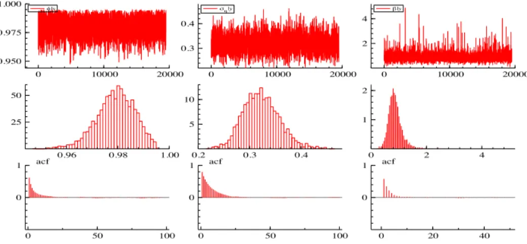
Figure 1 presents the information related to the estimation of the param-eters φ, ση2 and γ. The figure presents the MCMC sample, the histograms and the autocorrelation function based on 20,000 iterations. The first col-umn presents the results for φ|y, the second for ση|y and the third for
γ|y. 0 10000 20000 0.950 0.975 1.000 |y 0 10000 20000 0.3 0.4 |y 0 10000 20000 2 4 |y 0.96 0.98 1.00 25 50 0.2 0.3 0.4 5 10 0 2 4 1 2 0 50 100 0 1 acf 0 50 100 0 1 acf 0 20 40 0 1 acf
Figure 1. Graphs of the MCMC sample, histograms of the
posterior distributions of the parameters and the autocorre-lation function for a series generated without any outliers.
Figure 2 presents the simulated series at the top and the mean of the marginal posterior distribution of (δt|y), i.e., the probability that an
the posterior probability of the presence of an outlier. Because all the es-timated probabilities are smaller than 0.20 we do not detect any outlier in the simulated series even for values of c1 that are as small as 0.20.
0 100 200 300 400 500 600 700 800 900 1000 10 0 10 Returns 0 100 200 300 400 500 600 700 800 900 1000 0.25 0.50 0.75 1.00 P{t|y}
Figure 2. Results for the simulated series without outliers.
a) Simulated series. b) Posterior probability of the presence of an outlier estimated in step (1).
Simulated series with outliers:
We now insert LO and a volatility outlier (VO) in the data generating process. The VO is introduced in the volatility equation given in equation 1 as the following:
ht=µ+φ(ht−1−µ) +σηηt+δtVβtV,
whereδtV is an indicator function for the VO, andβtV is the size of the VO at the t-th observation.
We take the size of the LO as equal to the standard error of the simulated series without outliers multiplied by ∆, while the size of the VO is taken as equal to the standard error of the autoregressive process multiplied by Λ, i.e., Λ[σ2η(1−φ2)−1]0.5. Two isolated LOs were inserted, one of size 8 (∆ = 8) in the 50-th observation and another of size 5 in the 500-th observation. We also included six consecutive LOs of size 4 from the 250-th to the 255-th observation and one VO of size 5 in the 700-th observation. Because we used exactly the same sampled values for 0tsand ηt0s, the simulated series
with and without outliers are equal before the innovation outlier, i.e, up to the 699-th observation, except at the 50-th, from the 250 to the 255-th and at the 500-th observation, which are affected by additive outliers.
Figure 3 presents the simulated series in the upper part, and the esti-mated posterior probabilities of the presence of an outlier in step (7), i.e. estimated by the adapted algorithm, in the lower part. The posterior prob-abilities estimated in steps (1) and (7) are almost the same outside the blocks, and the probabilities found in step (1) inside the blocks are given in Table 1. 0 50 100 150 200 250 300 350 400 450 500 25 0 25 50 Returns 0 50 100 150 200 250 300 350 400 450 500 0.25 0.50 0.75 1.00 P{t|y} 550 600 650 700 750 800 850 900 950 1000 25 0 25 50 Returns 550 600 650 700 750 800 850 900 950 1000 0.25 0.50 0.75 1.00 P{t|y}
Figure 3. Results for the simulated series with outliers. a)
Simulated series. b) Posterior probability of the presence of an outlier.
In the first step, the two isolated outliers in the 50-th and 500-th obser-vations were detected as single outliers with a posterior probability almost equal to 1.0. Two blocks of width six each were detected, one from the
250-th to the 255-th observation and another from the 700-th to the 705-th observation. The first block matches 705-the positions of 705-the block of LOs introduced and the beginning of the second block is the position where the VO was introduced. The effect of a VO in the log volatility decreases exponentially, and the effect in the returns is multiplicative and given by the exponential of the effect on the log-volatility. In consideration of these facts it is not immediate to define an equivalent level effect. We just expect that the effect of and VO should decrease and eventually die out. It is interesting to note that not all of the posterior probabilities estimated in step (1) were large inside the blocks. After step (7), all of the estimated probabilities inside the LO block (see Table 1) are approximately equal to 1.0.In the second block, related to the VO, the posterior probability and the estimated size are decreasing, which is in agreement with the effect of a VO, as discussed previously. For all of the other observations, there was no false detection of an outlier with all of the posterior probabilities of the presence of an outlier smaller than 0.05.Thus, at least for these two simulated series the test had a good performance.
The estimates of the probability and the size (mean and standard de-viation of the posterior distribution) of the detected outliers are given in Table 1. Except for the observations with VO, we have the true size of the outlier. Table 1 presents the estimates of the size of the outlier by the stan-dard Gibbs sampler given in step (1) and by the adapted Gibbs sampler obtained in step (7). We can see that the standard Gibbs sampler yields good performance for isolated outliers, but that it is not as good for blocks of outliers. The adapted Gibbs sampler produces good estimates even when the outlier occurs in blocks and has a smaller standard deviation than the standard Gibbs sampler. We can see that the estimates are very close to a real value with all of the posterior probabilities near 1.0.We can say that the performance of the test is very good for the simulated series. In the following, all of the results are for the adapted Gibbs sampler.
4.2. New York Stock Exchange Composite Return Index. In this
subsection, we apply the outlier detection procedure to the NYSE compos-ite return (in percentages). The sample consists of 1,255 observations from January 2, 1997 and December 31, 2001. We will use this series to compare with the results of Zhang and King (2005).
The mean and standard deviation of the posterior distribution of the parameters φ, σ2
η and γ were equal to 0.940(0.006), 0.046(0.005) and
1.150(0.086), respectively.
Figure 4 presents the NYSE return series in the upper part, and the posterior probabilities of outliers estimated by the proposed method in the lower part.
Table 1. Estimation of the size of the outliers in the simu-lated series with outliers: the mean and standard deviation (in brackets) of the posterior distribution of the size of the outlier, and the mean of the posterior distribution of the presence of an outlier. The results are for the standard (step (1)) and adapted (step (7)) Gibbs sampler.
Outliers Standard Adapted Real Mean of the Posterior
GS GS Size distribution ∆50 8.0614 (0.9431) 8.0322(0.8431) 8 1.00 ∆250 4.6131 (0.8132) 4.0352(0.7683) 4 1.00 ∆251 2.6140 (0.3421) 3.9816(0.2667) 4 0.98 ∆252 2.8376 (0.3299) 4.0213(0.3134) 4 1.00 ∆253 4.9647 (0.4301) 4.0199(0.3353) 4 1.00 ∆254 3.2369 (0.7012) 4.0325(0.6831) 4 0.99 ∆255 3.7932 (0.4015) 4.3621(0.3421) 4 1.00 ∆500 5.1321 (0.2322) 5.0862(0.3262) 5 1.00 Λ700 8.2311 (0.3522) 3.9631(0.1793) IO 1.00 Λ701 7.4581 (0.3269) 3.8345(0.1622) IO 0.99 Λ702 7.2683 (0.3001) 3.6228(0.1766) IO 0.97 Λ703 5.7162 (0.2321) 2.6883(0.1492) IO 0.87 Λ704 5.5363 (0.2537) 2.6711(0.1539) IO 0.63 Λ705 4.021 (0.2251) (02.125.1498) IO 0.52
Table 2 gives the observations where the posterior probability of the presence of an outlier is larger than 0.5. The smallest value in Table 2 is 0.8976 and the largest posterior probability of observations not included in the Table 2 is very small, smaller than 0.1, except for three observations with probabilities in the interval (0.3,0.5). These results show that the method clearly classified whether we have an outlier at each observation of the series. The effect of the standard and adapted algorithm in the point estimates is not very large. For instance, the estimates for (φ, ση, β)
were equal to (0.935,0.192,1.21) when the model is estimated without out-liers, and were equal to (0.928,0.215,1.24) and (0.940,0.213,1.15) when the model is estimated with outliers using the standard and adapted methods, respectively.
0 50 100 150 200 250 300 350 400 450 500 5.0 2.5 0.0 2.5 5.0 NYSE 0 50 100 150 200 250 300 350 400 450 500 0.25 0.50 0.75 1.00 P(t| y) 550 600 650 700 750 800 850 900 950 1000 5.0 2.5 0.0 2.5 5.0 NYSE 550 600 650 700 750 800 850 900 950 1000 0.25 0.50 0.75 1.00 P(t| y) 1000 1020 1040 1060 1080 1100 1120 1140 1160 1180 1200 1220 1240 5.0 2.5 0.0 2.5 5.0 NYSE 1000 1020 1040 1060 1080 1100 1120 1140 1160 1180 1200 1220 1240 0.25 0.50 0.75 1.00 P(t| y)
Figure 4. Results for the NYSE series. a) Returns. b)
Table 2. Summary of the observations in which the poste-rior probability of the presence of an outlier is larger than 0.5., NYSE series
Date serial no. Return (%) posterior probability
20/10/97∗ 201 1.139 1.000 21/10/97∗ 202 1.567 0.981 23/10/97∗ 204 -1.847 0.994 27/10/97∗ 206 -6.791 0.974 28/10/97∗ 207 4.113 0.956 26/08/98∗ 415 -1.005 1.000 27/08/98∗ 416 -3.920 1.000 31/00/98∗ 418 -6.352 1.000 16/03/00 807 4.748 1.000 12/04/00∗ 826 -1.056 1.000 13/04/00∗ 827 -1.484 0.985 14/04/00∗ 828 -5.275 0.898 07/09/01∗ 1180 -1.948 0.977 17/09/01∗ 1182 -4.701 0.998 24/09/01∗ 1187 3.356 0.964 ∗
during or next crisis periods
To compare with the results from Zhang and King (2005), Table 3 presents the observations that are considered to be influential by those authors and/or by our analysis. Zhang and King (2005) used the slope and curvature local influence diagnostics, using three types of perturba-tions, volatility, additive and data perturbaperturba-tions, with a total of six tests, and they used a GARCH(1,1) model. The volatility perturbation is re-lated to VO, while the additive and data perturbations are rere-lated to LO. We use the corrected results that are available in X. Zhang home page in http://users.monash.edu.au/ xzhang/. The fourth column indi-cates whether the observation was detected as influential by any of the local perturbation tests. From the total of the 15 observations detected as outliers by our test, only two were not detected as outliers by any of the Zhang and King (2005) tests, the 206-th observation (27/10/97), which is in the middle of a patch of outliers related to the Asian crisis, and the 1187-th observation (25/09/01), which is near two other outliers and the 11-th September terrorist attack. From the 19 observations that were de-tected by any of the six local influential tests, only six were not dede-tected by our test, and none were during or near the crisis period. Among the six observations detected by the volatility perturbation tests (either by the slope- or curvature-based diagnostics), only one was not detected by our
test. Among the 15 detected by the additive perturbation, only three were not detected by our test, and among the 10 detected by the data perturba-tion tests, four were not detected by our test. Thus, we could say that the performance of the test was quite good and that it is able to detect all of the types of perturbations considered by Zhang and King (2005) with the advantage of using a single model, estimating the size of the outlier and giving evidence of the presence of the outlier. It is interesting to note that all of the main crises in the period, the Asian flu in October 1997, the Rus-sian cold in August 1998, the NASDAQ fall in April 2000 and the terrorist attack in September 2001, were detected as outliers. The only major crisis that was not detected as an outlier by our test was the Brazilian Sneeze in January 1999.
Table 3. Observations detected by the proposed test
sta-tistics and by the Zhang and King local influence tests. The fourth column shows whether the observation is detected by any local influence tests.
Type of local perturbation Patch Local Volatility Additive Data Date Serial no. test Perturb. Slope Curv. Slope Curv. Slope Curv.
02/09/97∗ 167 Y 20/10/97∗ 201 Y Y Y 21/10/97∗ 202 Y Y Y 23/10/97∗ 204 Y Y Y Y 24/10/95∗ 205 Y Y Y 27/10/97∗ 206 Y Y Y Y Y Y Y 28/10/97∗ 207 Y 27/08/98∗ 415 Y Y Y Y 28/08/98∗ 416 Y Y Y Y Y 31/08/98∗ 418 Y Y Y Y Y Y 15/10/98 450 Y Y 28/10/99 711 Y Y 04/01/00 757 Y Y 16/03/00 807 Y Y Y 12/04/00∗ 826 Y Y Y 13/04/00∗ 827 Y Y Y Y 14/04/00∗ 828 Y Y Y Y Y 16/05/01 1101 Y Y Y 07/09/01∗ 1180 Y Y Y 17/09/01∗ 1182 Y Y Y Y 25/09/01∗ 1187 Y total 15 18 5 4 7 9 5 6
∗during or next crisis periods
4.3. S˜ao Paulo Stock Exchange Return Index. In this last example,
we apply the outlier detection procedure to the IBOVESPA return series (in terms of percentages). The sample consists of 1,500 observations from
January 3, 1995 to December 27, 2000. The main crises in the period were the Mexican crisis in February and March, 1995, the Asian crisis in 1997 (June in Thailand, August in Indonesia and October in Hong Kong), the Russian Cold in August 1998 (including the LTCM crisis), the Brazilian Sneeze in 1999, and the NASDAQ fall in April 2000. The return series is presented in Figure 5.
The mean and standard deviation of the posterior distribution of the parameters φ, ση2 and γ, were equal to 0.979(0.009), 0.048(0.025) and 2.170(0.25), respectively. Figure 5 presents the IBOVESPA return series in the upper part, and the posterior probabilities of outliers estimated by the proposed method. 0 50 100 150 200 250 300 350 400 450 500 10 0 10 20 30 Ibovespa 0 50 100 150 200 250 300 350 400 450 500 0.25 0.50 0.75 1.00 P{t|y} 550 600 650 700 750 800 850 900 950 1000 10 0 10 20 30 Ibovespa 550 600 650 700 750 800 850 900 950 1000 0.25 0.50 0.75 1.00 P{t|y} 1050 1100 1150 1200 1250 1300 1350 1400 1450 1500 10 0 10 20 30 Ibovespa 1050 1100 1150 1200 1250 1300 1350 1400 1450 1500 0.25 0.50 0.75 1.00 P{t|y}
Figure 5. Results for the the IBOVESPA series. a)
Table 4 gives observations for which the posterior probability of the pres-ence of an outlier is larger than 0.5.The three smallest values in the table are 0.798,0.867 and 0.933, and the largest posterior probability of the ob-servations that are not included in the table is smaller than 0.1.Again, the method clearly classified whether we have an outlier at each observation in the series. Most of the influential observations detected were during or near to economic crises. It is interesting to observe that the pattern of the estimated posterior probability of the presence of an outlier during the Brazilian Sneeze crisis in 1999 is typical of a VO.
Table 4. Summary of the observations in which the
poste-rior probability of the presence of an outlier is larger than 0.5., IBOVESPA series
Date serial no. Return (%) posterior probability
10/01/1995 4 -10.47 0.9872 12/01/1995 6 9.22 0.9905 10/03/1995∗ 45 22.72 1.0000 26/10/1995 202 -6.84 0.9891 15/07/1997∗ 629 -8.99 1.0000 16/07/1997∗ 630 8.35 1.0000 17/07/1997∗ 631 -7.58 0.9695 18/07/1997∗ 632 -4.87 0.9334 27/10/1997∗ 703 -16.31 0.9840 28/10/1997∗ 704 6.14 0.9889 29/10/1997∗ 705 -6.30 0.9826 30/10/1997∗ 706 -10.42 0.9908 10/09/1998 921 -17.32 1.0000 11/09/1998 922 12.49 0.9861 15/09/1998 924 17.04 1.0000 14/01/1999∗ 1007 -10.59 1.0000 15/01/1999∗ 1008 28.73 1.0000 18/01/1999∗ 1009 5.21 0.9352 19/01/1999∗ 1010 3.59 0.8667 20/01/1999∗ 1011 3.81 0.7983 04/01/2000 1250 -6.67 0.9810 ∗
during or next crisis periods
5. Concluding remarks
We adapted the Justel et al. (2001) test to detect patches of outliers in the stochastic volatility model. We applied the suggested procedure to sim-ulated and real data sets. The test showed good performance when applied
to all the series. In the analysis of the simulated series, the estimation of the posterior probability inside the possible blocks improved the performance of the estimates of the size of the outlier and increased the posterior prob-ability of the presence of the outliers where they were introduced. This test was also applied to the NYSE series, which was analyzed by Zhang and King (2005) using six different tests, i.e., slope- and curvature-based diagnostics for three types of perturbations. The proposed test produced a similar result, showing power against different types of outliers with the advantage of estimating the size of the outlier and giving evidence of the presence of the outlier. The results of the application to the IBOVESPA series are also in agreement with the economic facts. In the four examples, the estimated probability in steps (1) and (7) were either small or close to 1.0, showing that the procedure is quite robust in relation to the choice of the critical values c1 and c2. This result and the robustness to the choice
of dwere verified in an analysis not reported here.
Acknowledgments: The authors would like to thank two anonymous
ref-erees for their helpful comments. The financial support from CNPq and FAPESP (00/10912-7, 13/00506-4) are gratefully acknowledged.
References
Andersen, T., Benzoni, L., Lund, J., 2002. An empirical investigation of continuous-time models for equity returns. J. Financ. 57, 1239-1284. Bates, D., 2000. Post-87 Crash fears in S&P 500 futures options. J.
Econo-metrics 94, 181-238.
Chen, C., Liu, L.-M., 1993. Joint estimation of model parameters and out-lier effects in time series. J. Am. Stat. Assoc. 88, 284–197.
Chib, S. 1995. Marginal likelihood from the Gibbs output. J. Am. Stat. Assoc. 90,1313-1321.
Chib, S., Nardari, F., Shephard, N., 2002. Markov chain Monte Carlo meth-ods for stochastic volatility models. J. Econometrics 108, 281–316. Chib, S.; Omori, Y., Asai, M., 2009. Multivariate stochastic volatility, in:
Mikosch, T., Kreiss, J-P., Davis, R.A., and Andersen,, T.G. (Eds), Hand-book of Financial Time Series. Springer Berlin Heidelberg, pp. 365-400,. de Jong, P., Shephard, N., 1995. The simulation smoother for time series
models. Biometrika 82, 339-350.
Durbin, J., Koopman, S.J., 2002. Simple and efficient simulation smoother for state space time series analysis. Biometrika 89, 603-616.
Eraker, B., Johannes, M., Polson, N. G., 2003. The impact of jumps in returns and volatility. J. Finance 53, 1269-1300.
Ghysels, E., A. C. Harvey, E. Renault, E., 1996. Stochastic volatility, in: Rao, C. R., Maddala, G. S. (Eds.), Statistical Methods in Finance. North-Holland, Amsterdam, pp. 119–191.
Harvey, A. C., Ruiz, E., Shephard, N., 1994. Multivariate stochastic vari-ance models. Rev. Econ. Stud. 61, 247–264.
Hotta, L. K., Tsay, R. S., 2012. Outliers in GARCH processes, in: Holan, S., Bell, W.R., McElroy, T. (Eds), Economic Time Series: Modeling and Seasonality (Festschrift David F. Findley). 337-358. Boca Raton, Fl.: Chapman & Hall/CRC Press.
Jacquier, E., Polson, N., Rossi, P. E., 2004. Bayesian analysis of stochastic volatility models with fat-tails and correlated errors. J. Econometrics 122, 185-212.
Justel, A., Pe˜na, D., Tsay, R. S. , 2001. Detection of outlier patches in autoregressive time series. Stat. Sinica 11, 651-673.
Kim, S., Shephard, N., and Chib, S., 1998. Stochastic volatility: likelihood inference and comparison with ARCH models. Rev. Econ. Stud. 65, 361– 393.
Kobayashi, M., 2006. Testing for volatility jumps in the stochastic volatility process. Asia-Pac. Finan. Markets 12, 143-157.
Liesenfeld, R., Richard, J. F., 2003. Univariate and multivariate stochastic volatility models: Estimation and diagnostics. J. Empir. Financ. 10, 505– 531.
Liesenfeld, R., Richard, J. F., 2006. Classical and Bayesian analysis of univariate and multivariate stochastic volatility models. Economet. Rev. 25, 335-360
McCulloch, R. E., Tsay, R. S., 1994. Bayesian analysis of autoregressive time series via the Gibbs sampler. J.Time Ser. Anal. 15, 235-250. Motta, A. C. O., Hotta, L. K., 2003. Exact maximum likelihood and
Bayesian estimation of the stochastic volatility model. Braz. Rev. Economet. 23, 183–226.
Nakajima, J., Omori, Y. , 2009. Leverage, heavy-tails and correlated jumps in stochastic volatility models. Computat. Stat. Data An. 53, 2335-2353. Omori, Y., Chib, S., Shephard, N., and Nakajima, J., 2007. Stochastic volatility with leverage: Fast and efficient likelihood inference. J. Econo-metrics 140, 425–449.
Pan, J., 2002. The jump-risk premia implicit in options: Evidence from an integrated time-series study, J. Finan. Econ. 63, 350.
Shephard, N., Pitt, M.K., 1997. Likelihood analysis of non-Gaussian mea-surement time series. Biometrika 84, 653-67. Correction (2004) 91, 249-50.
Tierney, L., 1994. Markov chains for exploring posterior distributions. Ann. Statist. 21, 1701-1762.
Tsay, R.S., Pena, D., Pankratz, A.E., 2000. Outliers in multivariate time series. Biometrika 87, 789–804.
van Dijk, D., Franses, P. H., Lucas, A., 1999. Testing for ARCH in the presence of additive outliers. J. Appl. Economet. 14, 539–562.
Zhang, X., 2004. Assessment of local influence in GARCH processes, J. Time Ser. Anal. 25, 301-313.
Zhang, X., King, M.L., 2005. Influence diagnostics in generalized autore-gressive conditional heteroscedasticity processes. J. Bus. Econ. Stat. 23, 118–129.