Evaluating Machine Learning Techniques for Smart Home Device Classification

(1)

Air Force Institute of Technology

AFIT Scholar

Theses and Dissertations Student Graduate Works

3-22-2019

Evaluating Machine Learning Techniques for Smart

Home Device Classification

Angelito E. Aragon Jr.

Follow this and additional works at:https://scholar.afit.edu/etd

Part of theDatabases and Information Systems Commons, and theInformation Security Commons

This Thesis is brought to you for free and open access by the Student Graduate Works at AFIT Scholar. It has been accepted for inclusion in Theses and Dissertations by an authorized administrator of AFIT Scholar. For more information, please [email protected].

Recommended Citation

Aragon, Angelito E. Jr., "Evaluating Machine Learning Techniques for Smart Home Device Classification" (2019).Theses and Dissertations. 2242.

(2)

EVALUATING MACHINE LEARNING TECHNIQUES FOR SMART HOME DEVICE CLASSIFICATION

THESIS

Angelito E. Aragon Jr., Captain, USAF

AFIT-ENG-MS-19-M-006

DEPARTMENT OF THE AIR FORCE AIR UNIVERSITY

AIR FORCE INSTITUTE OF TECHNOLOGY

Wright-Patterson Air Force Base, Ohio

(3)

The views expressed in this document are those of the author and do not reflect the official policy or position of the United States Air Force, the United States Department of Defense or the United States Government. This material is declared a work of the U.S. Government and is not subject to copyright protection in the United States.

(4)

EVALUATING MACHINE LEARNING TECHNIQUES FOR SMART HOME DEVICE CLASSIFICATION

THESIS

Presented to the Faculty

Department of Electrical and Computer Engineering

Graduate School of Engineering and Management

Air Force Institute of Technology

Air University

Air Education and Training Command

In Partial Fulfillment of the Requirements for the

Degree of Master of Science in Cyber Operations

Angelito E. Aragon Jr., B.S.C.E.

Capt, USAF

March 2019

DISTRIBUTION STATEMENT A.

(5)

EVALUATING MACHINE LEARNING TECHNIQUES

FOR SMART HOME DEVICE CLASSIFICATION

Angelito E. Aragon Jr., B.S.C.E. Capt, USAF

Committee Membership:

Barry E. Mullins, Ph.D., P.E. Chair

Brett J. Borghetti, Ph.D. Member

Timothy H. Lacey, Ph.D., CISSP Member

(6)

Abstract

Smart devices in the Internet of Things (IoT) have transformed the management of

personal and industrial spaces. Leveraging inexpensive computing, smart devices enable

remote sensing and automated control over a diverse range of processes. Even as IoT

devices provide numerous benefits, it is vital that their emerging security implications are

studied. IoT device design typically focuses on cost efficiency and time to market, leading

to limited built-in encryption, questionable supply chains, and poor data security. In a 2017

report, the United States Government Accountability Office recommended that the

Department of Defense investigate the risks IoT devices pose to operations security,

information leakage, and endangerment of senior leaders [1].

Recent research has shown that it is possible to model a subject’s pattern-of-life

through data leakage from Bluetooth Low Energy (BLE) and Wi-Fi smart home devices

[2]. A key step in establishing pattern-of-life is the identification of the device types within

the smart home. Device type is defined as the functional purpose of the IoT device, e.g.,

camera, lock, and plug. This research hypothesizes that machine learning algorithms can

be used to accurately perform classification of smart home devices.

To test this hypothesis, a Smart Home Environment (SHE) is built using a variety

(7)

bulbs, cameras, and smart plugs using Wi-Fi. In addition, a device classification pipeline

(DCP) is designed to collect and preprocess the wireless traffic, extract features, and

produce tuned models for testing. K-nearest neighbors (KNN), linear discriminant analysis

(LDA), and random forests (RF) classifiers are built and tuned for experimental testing.

During this experiment, the classifiers are tested on their ability to distinguish

device types in a multiclass classification scheme. Classifier performance is evaluated

using the Matthews correlation coefficient (MCC), mean recall, and mean precision

metrics. Using all available features, the classifier with the best overall performance is the

KNN classifier. The KNN classifier was able to identify BLE device types with an MCC

of 0.55, a mean precision of 54%, and a mean recall of 64%, and Wi-Fi device types with

an MCC of 0.71, a mean precision of 81%, and a mean recall of 81%. Experimental results

provide support towards the hypothesis that machine learning can classify IoT device types

(8)

Acknowledgements

To my family and friends: thank you for your unfailing support and encouragement

throughout this journey. I would not be where I am today without you.

To my advisor, Dr. Mullins: thank you for your mentorship throughout my time

here in AFIT. Your door was always open whenever I needed guidance.

To Dr. Borghetti, Dr. Lacey, and all AFIT faculty: thank you for sharing your time

and knowledge with me. I am grateful that I had the opportunity to learn so much from

your expertise and experience.

(9)

List of Figures

Figure Page

1. Wi-Fi Frame Fields [5] ... 6

2. BLE Architecture [6] ... 9

3. BLE Channel Map [6] ... 10

4. BLE States [6] ... 10

5. BLE Link-Layer Packet Structure [6] ... 12

6. BLE Data Packet ... 15

7. BLE Connection and Data Sending Diagram ... 16

8. Data Transmission [6] ... 19

9. GATT Client-Server Interaction [8] ... 20

10. GATT Structure [8]... 23

11. Netgear Nighthawk X4S R7800 router used as AP ... 34

12. Wi-Fi Access Point Settings ... 34

13. SHE Device Locations (not to scale) ... 38

14. Door Sensor Setup ... 39

15. Light Bulb Setup ... 40

16. Lock Setup ... 40

17. Plug Setup ... 41

18. Temperature Sensor Setup ... 41

(13)

20. Scanning and Sniffing Equipment. Plugable Bluetooth adapter (left), Alfa

AWUS036ACH Wi-Fi adapter (center), and Ubertooth One BLE sniffer (right) [29]–

[31] ... 43

21. Sniffer Layout ... 45

22. Commands to prepare Alfa card for data collection ... 46

23. Commands used to scan for Wi-Fi AP ... 47

24. Command used to scan for Wi-Fi devices associated to the AP... 48

25. Commands used to scan for BLE devices... 49

26. One-Hot Encoding ... 52

27. BLE Packet Length ... 61

28. BLE Link Layer Header Length ... 62

29. BLE Associated Packet Count ... 63

30. BLE RF Channels ... 63

31. BLE PDU Types ... 64

32. Wi-Fi Packet Length ... 66

33. Wi-Fi Vendors ... 66

34. Wi-Fi Associated Packet Count ... 67

35. Wi-Fi Packet Subtype ... 68

36. System under test diagram ... 70

37. A 𝒌𝒌𝒙𝒙𝒌𝒌 Confusion Matrix (𝒌𝒌= 𝟑𝟑) ... 72

38. Motion Source Appearance (left) and Location in SHE (right) ... 78

(14)

40. Confusion Matrices from BLE Door Sensors vs Temperature Sensors ... 90

41. Confusion Matrices from Wi-Fi Full-Featured Classification ... 92

42. Confusion Matrices from Wi-Fi Cameras vs Plugs ... 100

43. Confusion Matrices from Wi-Fi Classification (No Vendor Features) ... 100

44. BLE Door Sensors vs. Temperature Sensors Features ... 130

(15)

List of Tables

Table Page

1. Advertising PDU Types ... 14

2. Wi-Fi Devices ... 35

3. BLE Devices ... 36

4. Device Actions ... 37

5. Wi-Fi Vendor List ... 51

6. Wi-Fi Dataframe Columns ... 53

7. Wi-Fi Device Set Assignment ... 54

8. BLE Device Set Assignments ... 56

9. BLE Dataframe Columns ... 57

10. Hyperparameters used in Grid Search ... 59

11. Best-Performing Hyperparameters ... 60

12. Response Variables ... 73

13. Performance Metrics ... 76

14. Classifier Performance in BLE Full-Featured Classification ... 83

15. Device Type Precision in BLE Full-Featured Classification ... 85

16. Classifier Recall in BLE Full-Featured Classification... 85

17. Feature Importance in BLE Full-Featured Classification ... 87

18. Classifier Performance in BLE Best-3 Feature Classification ... 88

19. Classifier Performance in BLE Door Sensors vs Temperature Sensors ... 89

(16)

21. Device Type Precision in Wi-Fi Full-Featured Classification ... 93

22. Device Type Recall in Wi-Fi Full-Featured Classification ... 93

23. Feature Importance in Wi-Fi Full-Featured Classification ... 94

24. Classifier Performance in Wi-Fi Best-3 Feature Classification ... 95

25. Classifier Performance in Wi-Fi Cameras vs Plugs (Full-Featured Classification) . 97 26. Feature Importance in Wi-Fi Cameras vs Plugs (Full-Featured Classification) ... 97

27. Classifier Performance in Wi-Fi Cameras vs Plugs (Best Features Classification) . 98 28. Classifier Performance in Wi-Fi Classification (No Vendor Features) ... 99

29. Feature Importance in Wi-Fi Classification (No Vendor Features) ... 99

30. High and Low Performance BLE Classifiers ... 101

(17)

EVALUATING MACHINE LEARNING TECHNIQUES

FOR SMART HOME DEVICE CLASSIFICATION

I. Introduction

1.1 Background

Smart devices are increasingly being used in consumer and industrial applications.

Once connected to the Internet, these smart devices allow for remote sensing and control

of a wide variety of processes. The Internet of Things (IoT) is expected to have a network

of over 31 billion devices by 2020 [3]. IoT devices have the potential to affect personal

and commercial spaces, and therefore need to be studied for cybersecurity implications.

IoT device design often focuses on minimizing power and cost [4]. Such design decisions

can result in deficient security that cause information leakage. IoT devices regularly

perform automatic functions upon a subject’s arrival or departure. Traffic from these

devices can be analyzed to figure out a subject’s pattern-of-life [2]. By learning which

type of devices are activating upon a subject’s presence, a malicious actor can gain

exploitable information. Therefore, it is important to study whether such IoT device

classification is possible.

1.2 Problem Statement

Recent research has shown that it is possible to model a subject’s pattern-of-life

through data leakage from Bluetooth Low Energy (BLE) and Wi-Fi smart home devices

(18)

information wirelessly, available for malicious attackers to collect and analyze without user

awareness. A critical step in establishing pattern-of-life is the identification of the device

types within the smart home. Device type is defined as the functional purpose of the IoT

device, and extends across a broad spectrum including cameras, electrical plugs, light

bulbs, door locks, temperature sensors, and motion sensors. Previous techniques in IoT

device classification have been limited to manual packet analysis, a deliberate process that

requires specific knowledge of target devices. This research seeks to leverage machine

learning algorithms to produce a generalized and scalable method of IoT device

classification. The problem statement this work answers is whether machine learning can

be applied to successfully classify devices into their respective device types using collected

wireless traffic.

1.3 Hypothesis and Research Goals

This work hypothesizes that if machine learning classifiers are trained using

wireless traffic from a realistic smart home environment, then the classifiers can

successfully identify the device type of IoT devices to a high degree of accuracy.

The goals that guide this research are:

1. Design and build a source of realistic smart home device traffic.

2. Develop procedures to collect and prepare the wireless traffic for machine

learning classification.

3. Evaluate the performance of the linear discriminant analysis (LDA), k

(19)

4. Determine which features are most useful for classification purposes.

5. Assess the suitability of machine learning in IoT device type classification.

1.4 Approach

A smart home environment composed of commercially-available BLE and Wi-Fi

devices is assembled to produce authentic wireless traffic. The wireless traffic is collected

and preprocessed into a dataset suitable for machine learning. Classifiers are tuned and

trained. The models are tested on a number of classification tasks to evaluate their

performance. Results are synthesized to consider algorithm performance and device

security implications. The machine learning approach uses a multiclass classification

scheme, with three device types per wireless protocol used as response classes. K-nearest

neighbors, random forests, and linear discriminant analysis are the classification algorithms

used.

1.5 Assumptions/Limitations

The following assumptions and limitations are recognized throughout this

experiment:

• The devices selected in the smart home environment are representative of an authentic smart home.

• All devices are compatible with an Apple iPhone.

• All algorithms are accurately implemented by third-party libraries.

1.6 Contributions

This research adds to the fields of IoT security and machine learning classification

(20)

1. Smart Home Environment (SHE): A smart home architecture using BLE and Wi-Fi smart devices is designed to provide realistic wireless traffic that

can be used for analysis and classification.

2. Device Classification Pipeline (DCP): A system of machine learning techniques is applied to collect, process, and analyze the wireless traffic

produced by the smart home devices.

1.7 Thesis Overview

This thesis is organized into six chapters. Chapter 2 presents an overview of

relevant wireless protocols, machine learning techniques, classification algorithms, and

other related research. Chapter 3 provides the design details of the SHE and DCP systems

used to create, capture, prepare, and analyze the wireless traffic used in the experiment.

Chapter 4 discusses the experiment methodology, while Chapter 5 presents the analysis of

results. Lastly, Chapter 6 provides a summary of the work and considers possible avenues

(21)

II. Background and Related Research

2.1 Overview

This chapter presents a technical review of the wireless protocols Wi-Fi and BLE

in Sections 2.2 and 2.3 respectively to describe what features of their architecture and

packet structure are applied in machine learning classification. Section 2.4 follows with a

brief description of machine learning, and Section 2.5 provides a summary of traffic

analysis research, the current state of IoT device classification, and a discussion of related

research. Lastly, Section 2.6 offers a list of common terminology used throughout this

research.

2.2 Wi-Fi

By far, the most commonly used technology for wireless local area networks

(WLANs) is defined by the IEEE 802.11 standard, also known as Wi-Fi [1]. IEEE 802.11,

hereafter referred to as 802.11, defines the medium access control (MAC) and Physical

Layers (PHY). In wireless networks, a station (STA) is the addressable unit, and the basic

service set (BSS) is the fundamental building block of a WLAN. The BSS is the effective

area within which member STAs of the BSS can continue communication. In

infrastructure mode, WLAN topology is centered on an access point (AP) that connects

STAs from the WLAN to the wired network. A service set identifier (SSID) serves as the

primary name associated with a WLAN and is typically used by STAs to find WLANs.

Association is the process through which a STA connects to an AP. 802.11 expects

the AP to periodically send out beacon frames, containing the AP’s SSID and media access

(22)

the wireless channels defined in 802.11. Once an AP has been selected, the STA sends an

association request frame to the AP, and the AP responds with an association response

frame. After this process, the AP typically assigns an IP address to the STA through a

Dynamic Host Configuration Protocol (DHCP) exchange. Once completed, the STA has

joined the AP’s subnet and is viewed as simply another device in that subnet.

The general frame used to transmit data in 802.11 is illustrated in Figure 1. The

frame consists of various fields: frame control, duration/identification, address fields,

sequence control, frame body, and frame check sequence (FCS). The frame control field

contains the protocol version, frame type and subtype, and other control information. The

duration/identification field specifies the transmission time required for the frame. The

four address fields include the destination address, source address, receiver address, and,

occasionally, the transmitter address. The sequence control field helps identify duplicate

frames. The frame body, also known as the Data field, moves the higher-layer payload

between stations. The FCS is a checksum appended to the frame to detect corruption. If

the receiver calculates a different FCS than the FCS included in the frame, the frame is

deemed corrupted and is discarded.

Figure 1. Wi-Fi Frame Fields [5]

(23)

introduced in 2010 by the Bluetooth Core Specification 4.0 [7]. While classic Bluetooth

focuses on high data rates, BLE has been optimized for ultra-low power applications.

Bluetooth Low Energy is not trying to improve on Bluetooth classic; instead, it targets new

applications that have not previously used open wireless standards. These applications are

those that require devices to send minimal octets of data from once a second to once every

few days. By design, BLE is intended to minimize not only overall activity, but even the

time required to do anything useful. If a device is operating, even if it is nothing more than

checking whether it needs to send or receive something, it is using energy.

Certain key elements support low cost, including its industrial, scientific, and

medical (ISM) band, intellectual property license and low power. The 2.4 GHz ISM band

may have poor propagation, but is available worldwide with no license requirements. The

Bluetooth Special Interest Group (SIG) only requires a very low cost intellectual property

license. Finally, the best way to design a low-cost device is to reduce required materials

such as batteries. BLE was designed to work with the smallest, cheapest, and most readily

available battery option – button-cell batteries.

The BLE architecture is split into three parts: controller, host, and applications, as

shown in Figure 2. The controller is a physical device that transmits and receives radio

signals, and can convert these signals into packets with information. Within the controller

are the physical and link layers, as well as the lower half of the Host Controller Interface.

The controller can be identified as the Bluetooth chip or radio. The controller

communicates to other devices using an antenna, and to the host using the Host Controller

(24)

The host is a software stack that directs how multiple devices communicate with

one another, typically managing several services at the same time. The host controls the

Logical Link Control and Adaptation Protocol (L2CAP), the Security Manager Protocol,

Attribute Protocol, Generic Attribute Profile (GATT), and Generic Access Profile (GAP).

The L2CAP handles the passing of data between host and the controller through channels.

BLE uses three fixed channels: one each for connection management data, the Security

Manager, and the Attribute Protocol. The Security Manager Protocol handles device

pairing and key distribution. The Attribute Protocol defines the rules for accessing data by

another device through the use of attributes. The GATT resides above the Attributes

Protocol and defines the types of attributes and how they can be used. More detail on how

attributes work is included in Section 2.3.5. Lastly, the GAP controls how devices

discover, connect, and provide information to users in the application layer. It also outlines

the procedures needed to discover, connect, and pair with other devices by controlling the

link layer states. Finally, applications use the BLE architecture to provide various

(25)

Figure 2. BLE Architecture [6]

The physical layer of the controller transmits and receives bits using the 2.4 GHz

band. The frequency of the radio waves use a modulation scheme called Gaussian

Frequency Shift Keying (GFSK) that shifts the frequency slight up and down over a

Gaussian filter. Compared to classic Bluetooth’s 79 1-MHz channels, BLE is split into 40

separate channels, with a 2 MHz separation between one another, as shown in Figure 3.

Figure 3 also shows the advertising channels, indicated by the darkened channels. When

transmitting data, BLE transmits at the rate of 1 million bits per second (Mbps), with a

(26)

Figure 3. BLE Channel Map [6]

2.3.1 BLE Link-Layer States

The link layer describes packet details, advertising, and data channels. It also

describes how device discovery, data broadcasting, and connections operate. As shown in

Figure 4, the link layer defines five states: Standby, Advertising, Scanning, Initiating, and

(27)

Upon powering on, devices start in the standby state and remain there until the host

layers instruct them otherwise. Devices in the standby state can move into all other states.

Once fully powered, the advertising state can be initiated by the application through the

GAP. In the advertising state, the link layer can transmit advertising packets or respond to

scan requests. Devices that want to be discoverable or connectable must be in the

advertising state. Devices in the advertising state can only move to the connected or

standby state.

The scanning state allows a device to receive advertising channel packets from

other devices in the local area. There are two types of scanning: passive scanning and

active scanning. Passive scanning only receives advertising packets; the device never

transmits anything. In active scanning, the device additionally sends scan requests to all

advertising devices. The advertising device then replies with a scan response. Both the

scan requests and response packets are sent on the advertising channel.

To initiate a connection between devices, the link layer must go through the

initiating state. In this state, the initiating device listens for advertising packets from the

device with which it is trying to connect. Once an advertising packet is received, the link

layer sends a connect request to the advertising device and moves into the connected state.

The last state of the link layer is the connected state. The connected state can only

be entered through the advertising or initiating states. It is only in the connected state that

data channel packets are sent and received. There are two substates: master or slave. Only

the device that initiates the connection can become the master. A master device must

(28)

advertising state. The device that becomes the slave must have been advertising to another

device. A slave device can only transmit in response to the master device. Devices cannot

be both master and slave simultaneously, nor can a device be a slave of two masters at the

same time.

2.3.2 BLE Packet Structure

The packet is the standard data block of the link layer. There are two types of

packets: advertising and data packets. Advertising packets are used to find and connect to

other devices, while data packets are used once a connection is established. The packet

type is determined by the channel on which the packet is transmitted. If a packet is

transmitted on one of the three advertising channels, then it is an advertising packet; if it is

transmitted on any of the 37 data channels, it is a data packet.

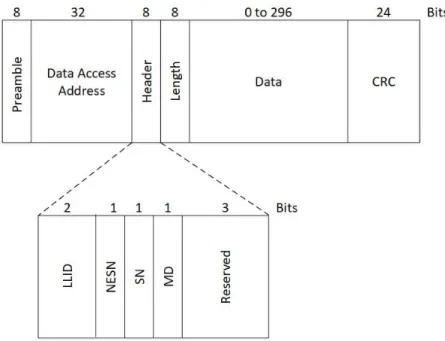
Link-layer packets follow the structure as displayed in Figure 5. These are divided

into the preamble, access address, header, length, data and cyclic redundancy check (CRC)

fields.

(29)

gain and determine the frequencies used for zero and one bits. The access address is the

next 32 bits and can be one of two types based on packet type: advertising access address

or data access address. Advertising access addresses are set at a fixed value

(0x8E89BED6) to help standardize the advertising process. Data channels use a different

random access address on each and every connection, which is used when data must be

reliably delivered to another device.

The header field varies based on the packet type. For advertising packets, the

header contains the advertising protocol data unit (PDU) type. Table 1 provides a summary

for each PDU type. ADV_IND indicates that the device is advertising as connectable

(available to create a connection) and undirected (not looking to connect to a specific

device); this is the advertising packet type most commonly used. ADV_DIRECT_IND

indicates that the device is connected and directed (looking for a specific device with which

to connect). ADV_NONCONN_IND indicates that the device is nonconnectable (refuses

to connect) and undirected; this is used by devices seeking to only broadcast data.

ADV_SCAN_IND, SCAN_REQ, and SCAN_RSP are used during active scanning.

ADV_SCAN_IND indicates that the advertising device is open to active scanning,

SCAN_REQ is a request made by the initiating device to receive a scan response, and

SCAN_RSP is the scan response itself. Lastly, the CONNECT_REQ header type is sent

by an initiating device to an advertising device when the initiating device wants to create a

connection. CONNECT_REQ packets contain information needed to establish a

(30)

Table 1. Advertising PDU Types

PDU Type Purpose

1 ADV_IND General advertising indication 2 ADV_DIRECT_IND Direct connection indication

3 ADV_NONCONN_IND Nonconnectable advertising indication 4 ADV_SCAN_IND Scannable indication

5 SCAN_REQ Active scanning request 6 SCAN_RSP Active scanning response 7 CONNECT_REQ Connection request

Data packets have headers containing the logical link identifier (LLID), sequence

number (SN), next expected sequence number (NESN), and more data, as shown in Figure

6. The LLID is used by the link layer to manage the channel for this connection. The

one-bit sequence number for each new data packet toggles from the previous data packet’s

sequence number, with the first data packet in a connection having a sequence number of

zero. The SN allows the receiving device to determine whether the received packet is a

retransmission of a previous packet or a new packet. The NESN allows for

acknowledgement of data packets. The last bit in the data packet header is the more data

bit, where 1 signals that there is more data to transmit, and 0 signals the end of the data

(31)

Figure 6. BLE Data Packet

The length field reports the size of the packet, with a range of valid values from 6

to 37 bytes for advertising packets, and 0 to 31 bytes for data packets. The payload is the

actual data that is being transmitted for use by the application. The final part of the packet

is a 3-byte CRC. The CRC is calcuated using the header, length and payload fields, and

serves to detect accidental changes to raw data.

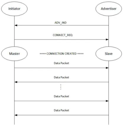
2.3.3 Creating Connections

A connection is required to reliably allow for two-way data transfer. Figure 7

shows how a connection is typically created. The first step is for one device to advertise

using an advertising packet (commonly with ADV_IND) and for another device to initiate

a connection to the advertising device with a CONNECT_REQ packet. Using the

(32)

devices, with the initiating device now the master device and the advertising device as the

slave device.

Figure 7. BLE Connection and Data Sending Diagram

All necessary information is contained within this CONNECT_REQ packet,

including access address, connection interval, and channel map. The access address is

randomly determined by the master. If a master has multiple slaves, it chooses a different

access address for each slave. When in a connection, the master must transmit a packet to

the slave once every connection event. The connection interval determines how frequently

this happens; the connection interval can be any period between 7.5 milliseconds to 4

(33)

for data traffic, and if the bit is set to zero, the channel is deemed a bad channel, and is

never used for data traffic.

The Generic Access Profile (GAP) defines the discovery and connection process

between devices. The GAP provides two types of discoverability: limited and general.

Limited-discoverable mode is used by devices that have just been made discoverable, and

are meant to stand out from general-discoverable devices. As such, devices are not allowed

to remain in the limited-discoverable mode for more than 30 seconds. The

general-discoverable mode is used by devices that are general-discoverable but have been inactive for a

period of time. This becomes the default mode for devices once they exceed the 30 seconds

allowed for limited-discoverable mode.

2.3.4 Sending Data

Once in a connection, devices can send data to each other using data packets. Data

packets have four fields in their header: logical link identifier, sequence number, next

expected sequence number and more data. The logical link identifer (LLID) determines

what kind of data the packet contains. The LLID can indicate that the packet is a link layer

control packet, which is used by the link layer to manage connections. Otherwise, it is a

data packet intended for the host, and can either be a start packet or continuation packet.

Start packets signal the beginning of a series of data packets, and continuation packets

make up the rest of the transmission. Interestingly, because the link layer does not need to

know the entire length of the data, continuation packets can be continuously sent. Data

packets have a single bit for the sequence number, beginning with zero for the first data

(34)

a data packet, the next expected sequence number (NESN) is used. If the data packet

received by a device has a sequence number of one, then the NESN is zero; otherwise, the

data packet would be retransmitted. Lastly, the MD bit indicates that the transmitting

device has more data ready to send. If one, then the receiving device maintains the

connection. If zero, then the two devices can close the connection to save power.

Figure 8 provides an example of how connection events occur between two

connected devices. A connection event is the start of a set of data packets sent from the

master to the slave and back again. Connection events are always initiated by the master

device. The master device initiates the transmission by sending a data packet with SN

zero, NESN zero, and MD one. The slave device receives this packet and attempts to send

its own packet, with SN zero, NESN one (acknowledging that the previous packet) and

MD one. However this packet was not properly received by the master device. Without an

acknowledgment from the slave device, the master device retransmits its first packet. The

slave device detects that retransmission of the previous packet is required, and does so.

This time, the packet is properly received. The master device no longer needs more data

from the slave device and sends a packet with the MD bit zero. The slave device

acknowledges this by sending its own packet with MD zero, and the connection event

between the two devices end. A second connection event is initiated by the master, but the

MD bit is set to zero. This type of connection event is typically performed to check on the

slave’s status, serving as a “ping”. The slave receives the packet, and seeing that MD is

(35)

Figure 8. Data Transmission [6]

2.3.5 Attributes

The Attribute Protocol, shown in Figure 2, is central to understanding Bluetooth

Low Energy. BLE is designed as a client-server architecture, where a server is a device

that has data, and a client is any device that is using data from another device. Figure 9

shows how the client-server architecture works. In practice, the master device acts as the

(36)

Figure 9. GATT Client-Server Interaction [8]

Attributes are the fundamental structure through which BLE achieves the

client-server architecture. The Generic Attribute Profile (GAP) is a set of rules that define how

to present, group, and transfer data using BLE. The GAP defines attributes as a piece of

labeled, addressable data, and each attribute has three parts: a handle, a type, and a value.

The attribute handle is the attribute’s 16-bit address. The attribute type is comparable to a

data type in programming languages, and is used to identify the nature of the attribute’s

information (e.g., temperature, pressure, time, etc.). Lastly, the attribute value is the actual

value and has a size between 0 to 512 bytes. Attributes are stored in an attribute database,

which is in turn contained within an attribute server. Clients communicate with the

attribute server to obtain desired information. There can only be one attribute server per

device, and every device must have both an attribute server and an attribute database.

Permissions must be set for every attribute in an attribute database, and these

permissions come in three categories: access, authentication, and authorization. Access

permissions must be set to readable, writable, or readable-writable. Authentication and

authorization permissions are not required and can be left open. The difference between

(37)

attribute value; any device has permission to view the attribute handles and types on a given

device.

The Attribute Protocol is the protocol through which clients find and access

attributes on an attribute server. It is a simple protocol with only six basic operations:

Request, Response, Command, Indication, Confirmation, and Notification.

A Request is sent by the client when the client wants the server to do an action and

send back a Response. A client can only send one Request at a time, and must wait for a

Response before sending another Request. A Command is similar to a Request, except no

Response is needed. Indications are used by the server to inform a client about an update

on a given attribute’s value, and require a Confirmation from the client. Notifications are

similar to Indications, except they need no Confirmation. Since Commands and

Notifications do not require Responses nor Confirmations, they can be sent without any

restrictions. If the receiving device cannot handle all the messages, the messages may be

dropped. Therefore, Commands and Notifications are unreliable, while Requests and

Indications are considered reliable.

Protocol messages are combinations of these basic operations used to perform

common tasks using the Attribute protocol. Their role is comparable to library functions

in programming languages. Most messages consist of both a Request and a Response

operation. For example, the Read Request message uses a Request operation that has a

handle of a desired attribute, and the Response returns the attribute value. Protocol

messages have a wide range of functionality that enable efficient reading, writing, error

(38)

For connected devices, the Generic Attribute profile (GATT) defines two basic

forms of grouping: characteristics and services. Figure 10 shows how the GATT structure

organizes characteristics and services. Characteristics are defined attribute types that can

only contain certain logical values. The BLE Specification provides over 200 predefined

characteristics such as Alert Status, Language, Battery Level, and Time Zone that can only

take on specific values based on their characteristic definition. A service is a collection of

characteristics and relationships with other services to perform a given function [9].

Sometimes refered to as profiles, services expose certain device information and

functionality in a standardized manner.

Predefined services include the Battery, Environmental Sensing, and Heart Rate

services [7]. For example, consider a personal fitness monitoring device that uses the

Battery, Environmental Sensing, and Heart Rate services. A user may connect the fitness

monitor to a smartphone through BLE. Through the Battery service, the user can monitor

the battery life of the device, ensuring that the device does not run out of power during

workout sessions. Through the Environmental Sensing service, the user can monitor

measurement data from the device’s various sensors, such as air temperature, humidity and

elevation. Finally, through the Heart Rate service, the user can track one’s heart rate

throughout the workout session. While predefined services accommodate common needs,

(39)

Figure 10. GATT Structure [8]

2.3.6 Security

The Security Manager (SM), shown in Figure 2, serves two fundamental functions:

device pairing and message authentication. These two functions enable the rest of BLE’s

security features. Pairing allows two unfamiliar devices to authenticate each other’s

identity in preparation for activity that requires security. During pairing, each device first

determines each other’s input and output capabilities (e.g., no input-no output, display only,

display yes/no, keyboard only, keyboard display) to determine what level of authentication

is possible. For example, if two devices are both display only, they would not be able to

authenticate via passkey entry, and the SM would default to simply letting the devices pair

automatically without authentication. After determining input and outputs, the SM then

proceeds to authenticate each other using a randomly-generated key, if possible. This is

often implemented by the user typing in a six-digit key. Lastly, keys are distributed

(40)

Authentication Code) algorithm, with the keys distributed using pairing. An additional

SignCounter value is used to prevent replay attacks.

2.4 Machine Learning

Coined by Arthur Samuel, the term machine learning (ML) refers to a field of

computer science that applies statistical techniques to give computers the capability to learn

from data without explicit programming [10]. ML plays a significant role in the fields of

statistics, data mining, and artificial intelligence. Machine learning is increasingly being

applied today to tasks too complex for traditional approaches or have no known algorithm

[11].

To illustrate, consider the task of distinguishing between different types of fruit.

Traditional approaches would need to first study the problem (for example, what is the

difference between an apple and an avocado) then write rules to solve the problem (apples

are red, avocados are green). However, this problem is more complex (some apples are

also green). Therefore, additional rules must be included to further refine the solution to

the program (apples have smooth skin, avocados have pebbled skin). But as more test

cases and situations are added, this set of rules grows significantly (watermelons are green

but have smooth skin), making the maintenance of these rules very difficult for a human

programmer.

A typical ML scenario seeks to predict an outcome measurement, usually

categorical (e.g., type of fruit) or quantitative (e.g., future house prices), using a set of

(41)

used to observe the outcome and feature measurements. With this data, a prediction model

is built to predict the outcome for new cases, or observations.

Given a sufficiently large dataset, machine learning excels in the type of problem

presented earlier. ML applies statistical techniques to reveal patterns within data. By

analyzing the data, an ML approach can develop a model using the patterns in the data, and

then produce a solution. Furthermore, the solution can reveal certain insights about the

data that may have been missed.

There are two broad types of machine learning: supervised learning and

unsupervised learning. Supervised learning requires the presence of the outcome

measurement, or labels, to direct the learning process. A typical supervised learning task

is classification, the task of assigning to which set of categories a given observation

belongs. In the fruit classification problem, the fruit type would be an example of a label,

and the task is assigning a fruit type to a given fruit.

As mentioned, classification is considered supervised learning because it requires

the presence of labels. Another supervised learning task is regression. Regression is the

task of predicting a numerical value for a given observation. An example is predicting

future house prices, given the features of house location and age. Because of the use of

labels, supervised learning methods can be evaluated on their performance. Chapter 3

provides the details on performance evaluation.

Unsupervised learning uses unlabeled data. Unsupervised learning aims to infer

the structure of data. A common task for unsupervised learning is clustering. The goal of

(42)

have not been clearly evident, and the detected groups may be used in applications such as

pattern recognition, compression, and graphics. An example of a clustering problem would

be when a website like Amazon or Netflix provides recommendations based on users’

browsing history [13]. By clustering items that are similar to those users have previously

looked at, online retailers or streaming services can suggest certain products or movies.

2.4.1 Classification Algorithms

The algorithms used in this experiment are among the most commonly used

machine learning classification algorithms. All three algorithms are identified as

supervised learning algorithms. Supervised learning requires the outcome measurement

to direct the learning process. In classification, the objective is to assign a given

observation to a particular class or label using a set of inputs or predictors. Because of

their use of outcome measurements, supervised learning algorithms may be evaluated on

their performance.

2.4.1.1K-Nearest Neighbors

K-Nearest Neighbors (KNN) classifies an observation by finding the observation’s

k nearest neighbors, where k is an integer, and classifying the observation to the class with

the highest estimated probability [14]. A commonly used distance metric is Euclidean

distance, however other distance metrics can be used, such as Manhattan distance or

Chebyshev distance. The hyperparameter k determines the number of neighbors KNN

considers in its classification of an observation. Supposing 𝑘𝑘= 3, KNN considers the three closest neighbors of 𝑥𝑥₀. The observation is assigned the majority class of these 𝑘𝑘

(43)

While this approach works well for data with unknown distributions, it leads to a higher

susceptibility to local anomalies within the data. Additionally, if there are many

dimensions in the data, several inputs may be “nearest” to the observation, leading to

reduced effectiveness.

2.4.1.2Linear Discriminant Analysis

Linear Discriminant Analysis (LDA) is a linear transformation technique first

proposed by Ronald Fisher in 1936. LDA models the distribution of the predictors

independently in each of the response classes, then applies Bayes’ theorem to find an

estimate of the posterior probability. A Gaussian or normal distribution is typically used

to model the distribution of the predictors. LDA assigns the observation to the response

class with the highest probability. When the assumption about the predictors’ distribution

does not hold, performance is reduced.

2.4.1.3Random Forests

A random forest is an ensemble of decision tree-based algorithms [14]. Decision

trees divide the feature space into different regions that can then be used to classify

observations. By using a multitude (or ensemble) of decision trees, random forests assign

an observation to the most commonly occurring class in the region to which it belongs. As

with a decision tree, there is a danger of overfitting when applying random forests.

2.5 Related Work

Wired network traffic analysis has been extensively studied. Preliminary methods

targeted port number and payload content analysis; these resulted in considerable success

(44)

Port number analysis is accurate only if networks adhere to port standards, and payload

analysis cannot cope with encrypted transmissions.

Transport-layer analysis has been applied to address the limitations of the previous

methods [17]. In peer-to-peer (P2P) networks where arbitrary ports are most commonly

used, transport-layer analysis allows the profiling of IP connection patterns. The

observation of source-destination IP pairs and IP address-port pairs offered a method of

studying P2P traffic without any examination of user payload. However, direct

transport-layer analysis can be time-consuming, and analytical scripts are restricted by programmer

knowledge.

Machine learning has emerged as a promising technique for traffic analysis [18].

Studies can be broadly categorized into unsupervised and supervised approaches. One of

the earliest studies using unsupervised learning, McGregor et al. applied clustering

techniques to group wired traffic flow between six common network protocols and found

that the data rate was a key feature in this effort [19]. Bernaille et al. used a variation of

the k-Means algorithm to classify Transmission Control Protocol (TCP) traffic to the

application type (e.g., file transfer protocol (FTP), hypertext transfer protocol (HTTP),

secure shell (SSH), etc.) using the packets at the start of traffic flow [20]. This approach

focused on the packets used during the TCP handshake and was able to classify traffic flow

with over 80% accuracy. However, this work assumed that the handshake can always be

captured at the onset of traffic flow, which is not always achievable. It was with Erman et

(45)

bi-and client-to-server. Their results showed that server-to-client datasets produced the

highest accuracy (95%), and that flow duration, number of bytes and number of packets

were the features that provided the most value in classifying packets.

Supervised learning introduced algorithms such as the k-Nearest Neighbors (kNN),

linear discriminant analysis (LDA), and quadratic discriminant analysis (QDA) to traffic

analysis. A study by Roughan et al. used these techniques to classify different network

applications to specific traffic classes [22]. The considered features were analyzed at the

packet level, flow level, and connection level. Packet level features were derived from

individual packets such as the size of the packet and the time the packet was sent. Flow

level features were derived from sequences of packets that shared common field values,

such as source IP address, destination IP address, and protocol type. Connection level

features were derived from transport-layer protocol information such as those found in TCP

connections. Of these features, average packet length and flow duration were found to be

the most valuable. Moore and Zuev were able to further improve on traffic classification

accuracy by using Naïve Bayes [23]. The dataset was manually classified beforehand, and

over 240 features were used to train the classifier. Using Naïve Bayes alone, the study

achieved approximately 65% accuracy. The classifier was then refined to reduce the

number of features, and accuracy was improved to over 95%. Auld et al. extended this

work by applying a Bayesian neural network (NN), further improving classification

accuracy [24]. The training NN achieved a classification accuracy up to 99% for data

trained and tested on the same day, and 95% for data trained and tested with an eight-month

(46)

of TCP PUSH packets, total number of bytes in the initial window (TCP handshake) from

client to server, and total number of bytes in the initial window (TCP handshake) from

server to client.

Wireless traffic adds a layer of complexity in traffic analysis. The most ubiquitous

wireless network standard, IEEE 802.11 (commonly known as Wi-Fi), uses encryption in

its wireless transmissions to protect against external eavesdropping. Nevertheless,

Atkinson showed that Wi-Fi can still leak private user information using only side-channel

information similar to those exploited in wired networks [25]. A Random Forests classifier

was trained on a dataset of Skype activity with around 60,000 observations and 600

features, and achieved around 97% accuracy. Furthermore, it was shown that a

classification accuracy of greater than 95% could be accomplished using only 200 variables

and 20 trees. The most valuable features were discovered to be the amount of time between

Sent frames, and the amount of time between a Received frame and the previous Sent

frame.

As for Internet of Things (IoT) devices, there is a shortage of wireless traffic

analysis in the current literature. This is likely due to the relative novelty of the IoT. A

study by Copos et al. analyzed two IoT devices, the Nest thermostat and Nest Protect smoke

detector, and succeeded in determining the devices’ Home and Away modes with 88% and

67% accuracy respectively [26]. Beyer expanded on the use of wireless traffic analysis by

showing that pattern-of-life profiling is possible using sniffed BLE and Wi-Fi traffic [2].

(47)

used frame size, measured in bytes, as a primary feature. Meidan et al. is the first study

found that applied machine learning to IoT device identification [27]. The goal of the study

was to determine whether a network device was a personal computer, a smartphone or an

IoT device. A dataset was produced using 802.11 wireless traffic from two PCs, two

smartphones, and ten IoT devices, with device types including baby monitors, refrigerators,

security cameras, thermostats, and smart outlets. A classifier was then trained using a

combination of gradient boosting and Random Forests techniques, and was able to classify

an IoT device with greater than 99% accuracy. A robust analysis on feature importance

was not performed. Wang et al. is the latest study to apply machine learning techniques to

traffic analysis of IoT devices [28]. A software-defined network (SDN) framework was

developed capable of efficient network quality-of-service management. This was achieved

through the use of deep-learning-based traffic analysis able to classify encrypted data

traffic to various applications (e.g., email, Skype video calls, Spotify music streaming,

etc.). Three deep-learning techniques were evaluated: multilayer perceptron, stacked

autoencoder, and convolutional neural networks.

2.6 Terminology

The following terms are frequently used throughout this thesis, and are defined here

for the purpose of clarity:

• Classification Algorithm/Classifier: a classification technique used to distinguish between response classes. The classification algorithms used in

this thesis are limited to k-nearest neighbors (KNN), linear discriminant

(48)

• Device Type: the broad functional purpose of an IoT device, e.g., cameras, smart plugs, locks. The device type is the response class the classifiers in

this thesis are attempting to identify.

• Response Class: the output of supervised classification classifiers. The response class referred to in this thesis is the device type.

• Test dataset: a subset of the dataset reserved to evaluate the classifier’s performance. The test dataset is never used to train the classifier.

• Training dataset: a subset of the dataset used to train the classifier.

2.7 Background Summary

This chapter provides a concise summary on the BLE and Wi-Fi protocols that IoT

devices use. It explains the underlying architecture of these protocols and how their

internal structure apply to machine learning classification. It offers a brief overview of

machine learning. It gives a brief survey into the background research on wired traffic

analysis and how machine learning has been applied in those efforts. While extensive

research has been done in traditional wired traffic, there is a current shortage on IoT traffic

analysis. This thesis contributes to the areas of IoT security and machine learning by

showing how classification techniques may successfully identify IoT devices using

(49)

III. System Design

3.1 Overview

This research offers two contributions in analyzing the classification of IoT devices

using wireless traffic analysis: a Smart Home Environment (SHE) and a Device

Classification Pipeline (DCP). SHE is a system of actual IoT devices that produces

authentic smart home traffic by integrating various BLE and Wi-Fi commercial devices in

one physical space. To study the wireless traffic produced by SHE, DCP is used to collect

and preprocess the wireless traffic into workable data, extract features from the data, and

produce tuned classifier models ready for testing. Lastly, data exploration is done to gain

an initial understanding of the original dataset before any classification is performed. This

chapter presents a detailed explanation of SHE, each component of DCP, and the products

of data exploration on the datasets.

3.2 Smart Home Environment (SHE)

SHE is designed to produce actual wireless IoT traffic for analysis. SHE consists

of a controller device, and a variety of BLE and Wi-Fi devices. Wireless traffic produced

by SHE is collected using sniffing equipment.

3.2.1 Controller

An iPhone 6S, using iOS version 12.1, serves as the central controller for all devices

in SHE. The iPhone controls a given device using the manufacturer-developed application.

All applications can be obtained via the App Store. When the user is within range of SHE,

the iPhone connects to the Internet via the Wi-Fi router and gains access to the devices in

(50)

connected through Bluetooth, the user can control the BLE devices using the device’s

application.

3.2.2 Wi-Fi Devices

To provide connectivity to Wi-Fi devices, a 2.4 GHz AP is set up with an SSID of

“yosemite" and Wi-Fi Protected Access II (WPA2) security. The AP used is a Netgear

Nighthawk X4S R7800 router, as shown in Figure 11. Figure 12 provides the list of AP

settings.

Figure 11. Netgear Nighthawk X4S R7800 router used as AP

(51)

All Wi-Fi devices, identified as 𝑤𝑤₂ - 𝑤𝑤₁₆, are connected to the AP. SHE contains five cameras, seven smart plugs, and three light bulbs across four different manufacturers.

Table 2 shows the list of Wi-Fi devices used in SHE, including details such as device type,

device manufacturer, device name, and MAC address. Device MAC addresses are found

by checking the labels on the physical device. Appendix A provides complete device

details, including a device’s model number and serial number.

Table 2. Wi-Fi Devices

ID Manufacturer Device Type Device Name MAC Address

𝑤𝑤1 Netgear Router Yosemite 78:D2:94:4D:AB:3E

𝑤𝑤2 Belkin Camera Netcam1 EC:1A:59:E4:FD:41

𝑤𝑤3 Belkin Camera Netcam2 EC:1A:59:E4:FA:09

𝑤𝑤4 Belkin Camera Netcam3 EC:1A:59:E5:02:0D

𝑤𝑤5 Dropcam Camera Dropcam 30:8C:FB:3A:1A:AD

𝑤𝑤6 TPLink Camera Kasa AC:84:C6:97:7C:CC

𝑤𝑤7 Belkin Plug Insight 14:91:82:24:DD:34

𝑤𝑤8 Belkin Plug Mini 60:38:E0:EE:7C:E5

𝑤𝑤9 Belkin Plug Switch1 14:91:82:CD:DF:3D

𝑤𝑤10 Belkin Plug Switch2 B4:75:0E:0D:94:65

𝑤𝑤11 Belkin Plug Switch3 B4:75:0E:0D:33:D5

𝑤𝑤12 Belkin Plug Switch4 94:10:3E:2B:7A:55

𝑤𝑤13 TPLink Plug TpPlug 70:4F:57:F9:E1:B8

𝑤𝑤14 Lifx Light Bulb Lifx1 D0:73:D5:26:B8:4C

𝑤𝑤15 Lifx Light Bulb Lifx2 D0:73:D5:26:C9:27

𝑤𝑤16 TPLink Light Bulb TpBulb B0:4E:26:C5:2A:41 3.2.3 BLE Devices

To control BLE devices 𝑏𝑏₁ - 𝑏𝑏₁₁ , the iPhone is used as a Bluetooth master device. SHE contains three locks, four door sensors, and four temperature sensors across five

(52)

environment, including details such as device type, device manufacturer, and device name.

Appendix A provides complete device details, including a device’s model number and

serial number.

Table 3. BLE Devices

ID Manufacturer Device Type Device Name

𝑏𝑏1 August Lock August1

𝑏𝑏2 August Lock August2

𝑏𝑏3 Kwikset Lock Kevo

𝑏𝑏4 BLE Home Door Sensor Home1

𝑏𝑏5 BLE Home Door Sensor Home2

𝑏𝑏6 Eve Door Sensor Door1

𝑏𝑏7 Eve Door Sensor Door2

𝑏𝑏8 Eve Temperature Sensor Room1

𝑏𝑏9 Eve Temperature Sensor Room2

𝑏𝑏10 Eve Temperature Sensor Weather

𝑏𝑏11 SensorPush Temperature Sensor Push 3.2.4 Device Actions

To produce sufficient traffic volume for machine learning, devices are set to

perform actions expected in a smart home environment. Actions can be programmed or

triggered. Programmed actions are set up by the user to occur on a scheduled time and

interval, while triggered actions are performed by devices upon an event. Events can occur

at any time during the experimentation. To reduce variability, devices of the same device

type are programmed to perform similar actions at identical times or events. Table 4 lists

(53)

Table 4. Device Actions

Device Name Device Type Actions Schedule/Event

1 Dropcam Camera Send email notification Motion detected 2 Kasa Camera Send email notification Motion detected 3 Netcam1 Camera Send email notification Motion detected 4 Netcam2 Camera Send email notification Motion detected 5 Netcam3 Camera Send email notification Motion detected 6 Lifx1 Light Bulb Turn on, Turn off Hourly, on the hour 7 Lifx2 Light Bulb Turn on, Turn off Hourly, on the hour 8 TpBulb Light Bulb Turn on, Turn off Hourly, on the hour 9 TpPlug Plug Turn on, Turn off Hourly, on the hour 10 Insight Plug Turn on, Turn off Hourly, on the hour 11 Mini Plug Turn on, Turn off Hourly, on the hour 12 Switch1 Plug Turn on, Turn off Hourly, on the hour 13 Switch2 Plug Turn on, Turn off Hourly, on the hour 14 Switch3 Plug Turn on, Turn off Hourly, on the hour 15 Switch4 Plug Turn on, Turn off Hourly, on the hour 16 Door1 Door Sensor Report door state Continuous 17 Door2 Door Sensor Report door state Continuous 18 Home1 Door Sensor Report door state Continuous 19 Home2 Door Sensor Report door state Continuous 20 August1 Lock Report lock state Continuous 21 August2 Lock Report lock state Continuous 22 Kevo Lock Report lock state Continuous 23 Room1 Temp Sensor Report temperature Continuous 24 Room2 Temp Sensor Report temperature Continuous 25 Weather Temp Sensor Report temperature Continuous 26 Push Temp Sensor Report temperature Continuous

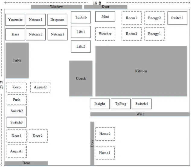
3.2.5 Device Location and Setup

All device locations are kept constant in SHE, except for the iPhone controller

which typically is on the user and is therefore not at a fixed location. Figure 13 shows the

location of each device in SHE. Wi-Fi devices are indicated by boxes with solid outlines,

(54)

a one-bedroom apartment with three doors, one set of large windows, a large table, and a

couch; these items are indicated by grey boxes. Devices locations are placed near power

outlets to reduce the need for additional power cords.

Figure 13. SHE Device Locations (not to scale)

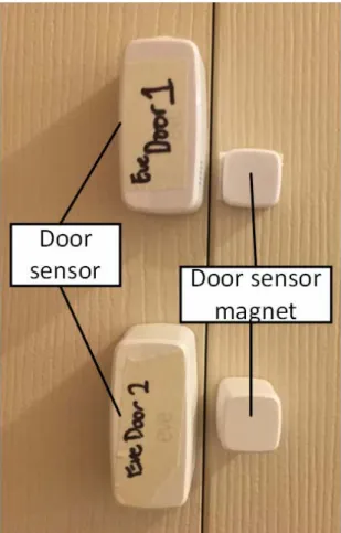
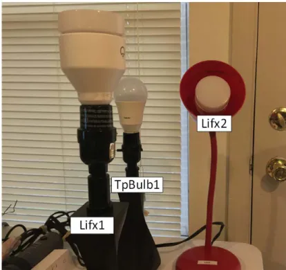
Figures 13 to 17 show how various devices are set up. Not all devices are shown

in the figures, but the overall configuration is similar across device types. Door sensors

(55)

door lock holders with actual door lock parts included. Plugs are installed into either power

strips or outlets, with no plugged-in device. Temperature sensors are placed in a flat

surface with open space around them. Cameras are placed around a motion source to

provide motion for their sensing capabilities. Figure 38 provides a photograph of the

camera device setup.

(56)

(57)

Figure 17. Plug Setup

(58)

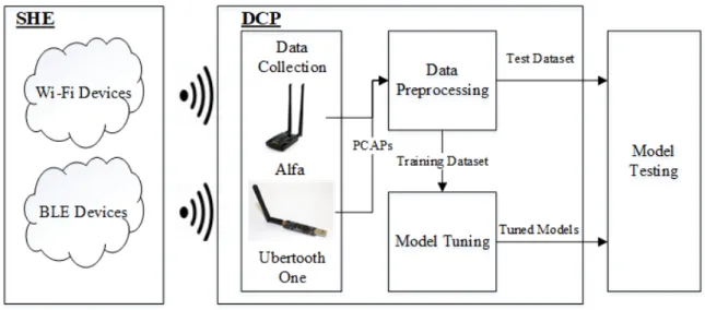
3.3 Device Classification Pipeline (DCP)

DCP is designed to collect and preprocess the wireless traffic into workable data,

extract features from the data, and produce tuned classifier models ready for testing. Figure

19 shows the DCP system diagram and its three components: (i) data collection, (ii) data

preprocessing, and (iii) model tuning. The outputs of DCP are tuned linear discriminant

analysis (LDA), k-nearest neighbors (KNN), and random forests (RF) classifiers for model

testing, as well as the test dataset. The following sections describe each component and

their functions.

Data collection is accomplished using user-inputted commands and scripts, as

described in Section 3.3.2, while data preprocessing and model tuning are accomplished

using the MulticlassDCP class written in Python. The MulticlassDCP class contains two sub-classes, BLEMulticlassDCP and WifiMulticlassDCP, one for each protocol.

(59)

3.3.1 Data Collection Hardware

A workstation is used to run all components of DCP. The workstation is an Acer

Aspire E15 with a 64-bit Intel Core i5-6200U 2.3 GHz processor, 8 GB DD4 RAM, 256

GB solid-state hard drive, and runs Kali Linux 2018.4 as the operating system. The

scanning and sniffing equipment consists of the Plugable Bluetooth adapter, three BLE

sniffers (Ubertooth One with firmware 2018-08-R1), and a long-range dual-band Wi-Fi

adapter (Alfa AWUS036ACH); all equipment is connected to the workstation using

Universal Serial Bus (USB). Each Ubertooth One sniffer uses a 2.4 GHz 2.2 dBi antenna,

while the Alfa card uses a 2.4 GHz and 5 GHz dual-band dipole antenna. Figure 20

provides images for these equipment.

Figure 20. Scanning and Sniffing Equipment. Plugable Bluetooth adapter (left), Alfa AWUS036ACH Wi-Fi adapter (center), and Ubertooth One BLE sniffer (right)

(60)

3.3.1.1Sniffer Distance Separation

All sniffers, Wi-Fi and BLE, operate in the 2.4 GHz band and must be horizontally

isolated to prevent interference. The required distance between antennae, 𝑑𝑑, to ensure horizontal isolation is given by the Fraunhofer distance equation

𝒅𝒅 ≥ 𝟐𝟐

𝑫𝑫_𝝀𝝀𝟐𝟐

(1) where 𝐷𝐷 is the antenna length in meters and 𝜆𝜆 is the wavelength of the device frequency band in Hz [32]. The Ubertooth One sniffers have 3.5 inch long antennae and operate at

an average wavelength of 2441 MHz, and the Alfa card has 6.5 inch long antennae and

operate at an average wavelength of 2412 MHz. Applying these values to (1) yields a

separation distance of about 5 inches for the Ubertooth One sniffers and 17 inches for the

Alfa card antenna. Separation distances are maintained by affixing the Ubertooth One

sniffers on a wooden board and ensuring that the Alfa card is located at an appropriate

distance, as shown in Figure 21.

3.3.2 Data Collection

Data collection supplies the raw data needed for data preprocessing. Data

collection occurs in two steps: scanning and sniffing. Scanning collects necessary

information required for sniffing and analysis, and sniffing gathers BLE and Wi-Fi wireless

traffic and stores them into packet capture files (pcap). The scanning and sniffing

Evaluating Machine Learning Techniques for Smart Home Device Classification

AFIT Scholar

Evaluating Machine Learning Techniques for Smart

Home Device Classification

AIR FORCE INSTITUTE OF TECHNOLOGY

Abstract

Acknowledgements

Table of Contents

List of Figures

List of Tables

I.

Introduction

II.

Background and Related Research

III.

System Design

𝒅𝒅 ≥ 𝟐𝟐