Toward a General-Purpose Heterogeneous Ensemble for Pattern Classification

(1)

Original Citation:

Toward a General-Purpose Heterogeneous Ensemble for Pattern Classification

Hindawi Publishing Corporation Publisher:

Published version: DOI:

Terms of use: Open Access

(Article begins on next page)

This article is made available under terms and conditions applicable to Open Access Guidelines, as described at http://www.unipd.it/download/file/fid/55401 (Italian only)

Availability:

This version is available at: 11577/3169491 since: 2015-12-14T18:00:09Z

10.1155/2015/909123

(2)

Research Article

Toward a General-Purpose Heterogeneous Ensemble for

Pattern Classification

Loris Nanni,

1

Sheryl Brahnam,

2

Stefano Ghidoni,

1

and Alessandra Lumini

3 1_{DEI, University of Padova, Via Gradenigo 6, 35131 Padova, Italy}

2_{Computer Information Systems, Missouri State University, 901 S. National, Springfield, MO 65804, USA} 3_{DISI, Universit`a di Bologna, Via Sacchi 3, 47521 Cesena, Italy}

Correspondence should be addressed to Stefano Ghidoni; [email protected] Received 9 April 2015; Accepted 27 July 2015

Academic Editor: Reinoud Maex

Copyright © 2015 Loris Nanni et al. This is an open access article distributed under the Creative Commons Attribution License, which permits unrestricted use, distribution, and reproduction in any medium, provided the original work is properly cited. We perform an extensive study of the performance of different classification approaches on twenty-five datasets (fourteen image datasets and eleven UCI data mining datasets). The aim is to find General-Purpose (GP) heterogeneous ensembles (requiring little to no parameter tuning) that perform competitively across multiple datasets. The state-of-the-art classifiers examined in this study include the support vector machine, Gaussian process classifiers, random subspace of adaboost, random subspace of rotation boosting, and deep learning classifiers. We demonstrate that a heterogeneous ensemble based on the simple fusion by sum rule of different classifiers performs consistently well across all twenty-five datasets. The most important result of our investigation is demonstrating that some very recent approaches, including the heterogeneous ensemble we propose in this paper, are capable of outperforming an SVM classifier (implemented with LibSVM), even when both kernel selection and SVM parameters are carefully tuned for each dataset.

1. Introduction

The present trend in machine learning is focused on building optimal classification systems for very specific, well-defined problems. Another research focus, however, would be to work on building General-Purpose (GP) systems that are capable of handling a broader range of problems as well as multiple data types. Ideally, GP systems would work well out of the box, requiring little to no parameter tuning but would still perform competitively against less flexible systems that have been optimized for very specific problems and datasets. One promising avenue of exploration is to build ensembles that are composed of diverse classifiers that merge their hypotheses [1], thereby resulting in a better approximation of a true hypothesis [2].

Many ensemble construction techniques are available. One approach is to perturb the information that is given to the base classifiers. The basic assumption behind this approach is that each of the base classifiers makes errors that are independent of each other, but as part of an ensemble they offer stronger classificatory power. To build an ensemble using this approach,𝐾training sets are first created, and𝐾

classifiers are then trained on each of the𝐾 training sets. The results of the 𝐾 classifiers are combined using some decision rule such as majority voting, sum rule, max rule, min rule, product rule, median rule, and Borda count. Different types of perturbations methods have been developed to max-imize the classifier diversity in an ensemble. These methods focus on perturbing the training patterns, the feature sets, the classifiers, or some combination of these perturbation methods.

In pattern perturbation,𝐾new training sets are created (commonly following an iterative approach) by perturbing the original training set, and a different classifier is trained on each new set. Some well-known pattern perturbation techniques include Bagging [3], Arcing [4], Class Switching [5], and Decorate [6]. In Bagging [3], new training sets are subsets of the original training data. In Arcing [4], each new training set is created based on the misclassified patterns in the previous iteration. In Class Switching [5], new training sets are created by randomly changing the labels of a subset of the original training data. Decorate [6] creates new training sets by adding artificial patterns misclassified by the combined decision of the ensemble.

Volume 2015, Article ID 909123, 10 pages http://dx.doi.org/10.1155/2015/909123

(3)

Feature perturbation techniques manipulate a set of orig-inal features into new training sets composed of perturbed features. Some important examples of feature perturbation include random subspace (RS) [7] and Input Decimated Ensemble [8]. In RS [7],𝐾new training sets are randomly generated from subsets of the feature set. In Input Decimated Ensemble [8], new training sets are generated using the principal component analysis (PCA) transform, where PCA is calculated on the training patterns belonging to each particular class. The ensemble size is thus bounded by the number of classes. This limitation can be avoided, however, as shown in [9], if PCA is performed on training patterns that have been partitioned into clusters.

New ensembles can also be composed by mixing the two perturbation methods discussed above. For example, Random Forest [10] uses a bagging ensemble of decision trees, where a random selection of features is used to split a given node.

Finally, in classifier perturbation, each classifier of the same type (homogeneous ensembles) can be given differ-ent parameter values, or differdiffer-ent classifiers (heterogeneous ensembles) can be combined and trained on the same training set. Classifier perturbation methods for building ensembles have been the least studied in the literature, but recently several studies have focused on this type of ensemble [11]. Moreover, several papers have investigated building GP heterogeneous ensembles [12, 13]. In [12], an ensemble combining the RS approach with an ensemble using an editing approach to reduce outliers was compared with other state-of-the-art methods across sixteen benchmark datasets representing very different problems (numerous medical problems, image problems, a vowel dataset, a credit dataset, etc.). Although none of the ensembles investigated in [12] worked consistently well across all sixteen datasets, one GP ensemble worked well across all the image datasets. Moreover, in some cases, the GP ensemble performed better than an SVM whose parameters had been optimally tuned on a specific dataset.

GP ensembles that exploit information available in dif-ferent feature extraction methods and representations of the data have also been explored. In [13], for instance, the goal was to search for a GP ensemble for protein classification that combined an optimal set of different protein representations and descriptors and that performed well across fourteen protein classification datasets representing different protein classification tasks. It was discovered in [13] that large descriptors work better when a large training set is available (due to the curse of dimensionality). Although no ensemble was discovered that provided the best performance across all fourteen datasets, it was shown that it is always possible to find a more limited GP ensemble that performed well across each type of dataset.

In this work the focus is on testing different classifiers and their combinations across twenty-five datasets (fourteen image datasets and eleven UCI data mining datasets). In the image datasets, two state-of-the-art texture descriptors are utilized: Local Ternary Patterns [14] and Local Phase Quantization [15]. As the majority of machine learning papers published in the literature are based on the LibSVM

implementation of SVM, the aim of this work is to com-pare the performance of the LibSVM library with several recently proposed classifiers (Gaussian process classifiers, RS of AdaBoost, RS of rotation boosting, and deep learning) and to show that a heterogeneous GP ensemble of classifiers works well across the different datasets. For all the classifiers compared in this study, we use well-known toolboxes that have been extensively tested and that are freely available. Moreover, to make results reproducible and to gain a wider diffusion of this type of research, the MATLAB code/interface for building the GP heterogeneous ensembles proposed in this work is provided. We hope this tool will also prove useful for practitioners.

The most interesting result obtained from our experi-ments is that the best GP ensemble proposed in this paper outperforms each stand-alone classifier without any ad hoc tuning on the dataset: the same fusion rule is used for all twenty-five datasets tested in this work. As a result, we are confident that the proposed GP ensemble can easily be extended to other problems and should prove useful to researchers who want a reliable classifier that works well without tuning it. It should be noted, however, that there is a cost associated with using heterogeneous ensembles: increased computational time.

The remainder of this paper is organized as follows. In Section2, the different classifiers explored in this paper are briefly described. In Section 3, the feature descriptors are outlined. In Section4, we provide an overview of the twenty-five datasets. In Section 5, we present the experimental results along with our best GP heterogeneous ensembles. We conclude in Section 6 with a few reflections and remarks on some issues involved in developing GP ensembles and list some future directions of research. The MATLAB code for all the classifiers used in the proposed ensembles are available at https://www.dei.unipd.it/node/2357. Moreover, for the purpose of reproducing and comparing results, the split training/testing sets are also available at the above website.

2. Classifiers

Since the aim of this study is to find a heterogeneous multiclassifier system that works well with a large number of datasets, we examined the fusion by sum rule of several state-of-the-art classifiers: the Support Vector Machine (SVM), Gaussian process classifier (GPC), RS of AdaBoost (RS AB), RS of rotation boosting (RS RB), and deep learning (DL). The sum rule [2] simply sums the matching scores (normalized to mean 0 and standard deviation 1) provided by each of the different classifier systems. Each of the classifiers examined in this study is described briefly below.

2.1. Support Vector Machine (SVM). SVM [16] is a binary classifier and is used as the core classifiers in several of our ensembles. An SVM performs classification by cutting the 𝑛-dimensional space (𝑛being the number of features) into two regions associated with two distinct classes, often referred to as the positive class and thenegative class. The regions are separated by an𝑛-dimensional hyperplane that

(4)

has the largest possible distance𝑑from the training vectors of the two classes. Three kernels are tested in our exper-iments: linear, radial basis function, and polynomial. For each kernel, a dataset driven fine-tuning of parameters is performed. SVM is implemented using LibSVM, available at http://www.csie.ntu.edu.tw/∼cjlin/libsvm/.

In addition to SVM implemented with LibSVM, we test an RS ensemble with SVM as the classifier (using fifty different subspaces that include 50% of the original features). This ensemble is called RS SVM.

2.2. The Gaussian Process Classifier (GPC). GPC [17] is a probabilistic approach for learning in kernel machines. It considers two procedures for approximating inference for binary classification: (1) Laplace’s approximation, which is based on an expansion around the mode of the poste-rior, and (2) the Expectation Propagation algorithm, which is based on matching moments approximations to the marginals of the posterior. GPC is implemented using the MATLAB code available athttp://www.gaussianprocess.org/ gpml/code/matlab/doc/index.html.

2.3. Random Subspace of AdaBoost (RS AB). RS AB [18] is a supervised learning algorithm that boosts the classification performance of a simple binary classifier by combining a collection of weak classifiers. The output of the weak learners is combined into a weighted sum that represents the final output of the boosted classifier. In this work, we combine AdaBoost with the RS method [7] for building ensembles. This results in a pseudorandom selection of subsets of components in the feature vector that are then used for training the different classifiers of the ensemble. We use RS to construct fifty different subspaces that include 50% of the original features. A different AdaBoost.M2 [18] is trained on each subspace. AdaBoost.M2 gives the weak learner (a neural network in our studies) more expressive power. The 50 classifiers are combined by sum rule.

2.4. Random Subspace of Rotation Boosting (RS RB). RS RB is the random subspace version of rotation boosting (RB). RB [19] is an ensemble of decision trees based on randomly splitting the feature set into subsets. In each subset a feature transform is applied (PCA without feature reduction in the original version of RB). Instead of PCA, the feature transform used in this study is Neighborhood Preserving Embedding (NPE) as in [9]. NPE is described in Section3.3.

2.5. Deep Learning (DL). Deep learning is a recent and one of the best-performing approaches to Artificial Intelligence, a field that was revolutionized when it was first proposed in 2006 [20]. The main feature of deep learning is its layered structure: there are several layers of processing nodes between its input and output, with every layer adding a certain level of abstraction to the overall representation. For example, image interpretation is a task that can be performed through several steps: at a lower level, small image patches are considered, leading to features like edges and texture. Such low-level descriptors can be combined together to build a more complex representation: at the second level,

for example, features like larger image patches and contours can be considered. Moving toward upper levels, the elements considered by the network are of increased complexity and are extracted from larger areas in the image (i.e., larger sets of input data).

Another major feature of deep learning networks is that they are able to exploit unlabeled data, a crucial feature when dealing with huge sets of data. Deep learning has been widely used in computer vision and image understanding applications, including object recognition in 3D (RGB-D) data [21] and face detection and verification [22].

In this work, we test the deep learning approach based on the Feedforward Backpropagation Neural Network (FBNN) [23] with a sigmoid activation function. We train FBNN for 10000 epochs with minibatches of size 25. Three versions of DL are tested DL1, DL2, and DL3. Each has an input layer that is the size of the input feature vector and an output layer that is the size of the number of classes. DL1 has a hidden layer of size 100. DL2 has two hidden layers each of size 100, and DL3 has two hidden layers each of size 500. DL is implemented using the MATLAB code available at http://it.mathworks.com/ matlabcentral/fileexchange/38310-deep-learning-toolbox.

3. Feature Extraction

In Sections3.1and3.2, we briefly describe the texture features used with the fourteen image datasets. Many methods are available for extracting features from texture. Two of the best-performing methods are Local Ternary Patterns (LTP) and Local Phase Quantization (LPQ). In Section3.3, we describe the NPE descriptor that is used as a transform in RS RB.

3.1. Local Ternary Patterns (LTP). LTP [14] is an extension of the canonical Local Binary Pattern (LBP) operator designed to be more discriminant and less sensitive to noise in uniform regions. The LBP operator [24] is computed at each pixel𝐼_𝑐of an image by considering the differences between grey-level values of a small circular neighborhood (with radius𝑅pixels):

LBP(𝑃, 𝑅) =

𝑃−1 ∑ 𝑖=0

𝑠 (𝐼_𝑝− 𝐼_𝑐) 2𝑖, (1) where𝑃is the number of pixels in the circular neighborhood

𝐼_𝑝and𝑠(𝑥)is a threshold function such that

𝑠 (𝑥) = {1, 𝑥 ≥ 0

0, 𝑥 < 0. (2)

In the LTP, the threshold function𝑠(𝑥)is substituted by a ternary coding function that makes the operator more robust to noise.

The ternary coding𝑡(𝑥)is defined as

𝑡 (𝑥) = { { { { { { { 1, 𝑥 ≥ 𝜏 0, |𝑥| ≤ 𝜏 −1, 𝑥 ≤ −𝜏, (3)

(5)

The ternary code obtained by the𝑡(𝑥)function is split into two binary codes by considering its positive and negative components, according to the following binary function

𝑏_V(𝑡(𝑥)):

𝑏_V(𝑡 (𝑥)) ={_{ {

1 𝑡 (𝑥) =V

0 otherwise V∈ {−1, 1} . (4) Thus, the LTP_Voperator forV∈ {−1, 1}is

LTP_V(𝑃, 𝑅) =

𝑃−1 ∑ 𝑝=0

𝑏_V(𝑡 (𝐼_𝑝− 𝐼_𝑐)) 2𝑛. (5) The resulting binary codes are used to create two his-tograms of LTP values.

In this work two values of𝑅and𝑃are used: (𝑅 = 1;𝑃 =

16) and (𝑅 = 2,𝑃 = 16); hence, we have four codes (two sets of parameters, with a positive and a negative code for each of them).

3.2. Local Phase Quantization (LPQ). LPQ is a texture descriptor [15] based on the blur invariance of the Fourier Transform Phase. For each pixel positionx of the image𝑓(x), the 2D short-term Fourier transform (STFT) is computed over a rectangular neighborhood of size𝐿 × 𝐿, and four com-plex coefficients, corresponding to the 2D frequencies, are considered and quantized to construct the final descriptor:

𝑢₁ = [𝑎, 0]𝑇_,_𝑢

2 = [0, 𝑎]𝑇,𝑢3 = [𝑎, 𝑎]𝑇, and𝑢4 = [𝑎, −𝑎]𝑇,

where𝑎is a scalar frequency parameter.

The four complex coefficients[𝑢₁, 𝑢₂, 𝑢₃, 𝑢₄]need to be decorrelated before quantization to become statistically inde-pendent and maximally preserve the information. Assuming a Gaussian distribution and a fixed correlation coefficient between adjacent pixel values 𝜌, a whitening transform can be obtained from the singular value decomposition of the covariance matrix of the transform coefficient vector. After decorrelation, the vector𝐺_𝑐 ∈ R8 that contains the decorrelated STFT coefficients for the pixel𝐼_𝑐 is quantized using a scalar quantizer𝑠(𝑥) (already defined in(2)). Then the final LPQ code is represented as an integer between 0 and 255 using the binary coding:

LPQ(𝐿) =

8 ∑ 𝑖=1

𝑠 (𝐺_𝑐) 2𝑖−1. (6) Finally, a histogram of these integer values is composed and used as a feature vector. In this work, we tested LPQ using two sizes for the local window𝐿(3 and 5), both with Gaussian derivative quadrature filter pairs for local frequency estima-tion. LPQ is implemented using the MATLAB code available athttp://www.cse.oulu.fi/CMV/Downloads/LPQMatlab.

3.3. Neighborhood Preserving Embedding (NPE). First, pro-posed in [25], the NPE transformation is a global approach that preserves the local neighborhood structure on the data manifold. PCA, in contrast, preserves the global Euclidean structure. Thus, NPE is less sensitive to outliers than PCA.

As described in Section2, we use NPE as the transform for dimensionality reduction in RB.

Given a set of points𝑥₁, 𝑥₂, . . . , 𝑥_𝑚∈ 𝑅𝑛, the idea behind NPE is to find a transformation matrixA that maps these points into another set𝑦₁, 𝑦₂, . . . , 𝑦_𝑚 ∈ 𝑅𝑑, where𝑑 ≪ 𝑛.In this way,𝑦_𝑖= 𝐴𝑇𝑥_𝑖represents𝑥_𝑖in a space with significantly less dimensions.

NPE begins by building a weight matrix to describe the relationships between data points: each point is described as a weighted combination of its neighbors. An optimal embedding is sought such that the neighborhood structure is preserved in the reduced space.

The algorithm can be formalized in three steps:

(1) Build an adjacency graph: define a graphG with𝑚 nodes. The𝑖th node represents the point𝑥_𝑖. There is an edge between𝑖and𝑗if and only if𝑥_𝑗is one of the

𝐾nearest neighbors of𝑥_𝑖.

(2) Compute weights: in this step weights on edges are calculated. W is the weight matrix and 𝑤_𝑖𝑗 is the weight of the edge from node 𝑖 to node 𝑗. The matrix can be computed by minimizing the objective function: min 𝑚 ∑ 𝑖 󵄩󵄩󵄩󵄩 󵄩󵄩󵄩󵄩 󵄩󵄩󵄩𝑥𝑖− 𝑚 ∑ 𝑗 𝑤_𝑖𝑗𝑥_𝑗󵄩󵄩󵄩󵄩󵄩󵄩󵄩󵄩 󵄩󵄩󵄩 2 Subject to: 𝑚 ∑ 𝑗 𝑤_𝑖𝑗= 1, 𝑗 = 1, 2, . . . , 𝑚. (7)

(3) Compute the projection: in this step the linear projec-tion is computed. The following eigenvector problem is solved:𝑋𝑀𝑋𝑇a= 𝜆𝑋𝑋𝑇a;𝑀 = (𝐼 − 𝑊)󸀠(𝐼 − 𝑊). The local manifold structure is then preserved using the following transformation matrixA that maps𝑥_𝑖 to𝑦_𝑖:

𝑦_𝑖=A𝑇𝑥_𝑖, where A = (a₀,a₁, . . . ,a_𝑑−1) . (8)

4. Datasets

To assess their generalizability, the approaches proposed in this paper were tested across twenty-five datasets: fourteen image classification datasets and eleven UCI data mining datasets.

4.1. Image Classification Datasets. The following fourteen image classification datasets that represent very different computer vision problems were selected to evaluate the generalizability of our approach:

(i) PS: this Pap Smear dataset [26] contains 917 images representing cells that are used in the diagnosis of cervical cancer.

(ii) VI: this dataset, reported in [27], contains images of viruses. A split training/testing set is provided by the authors and is used in this paper. The masks for subtracting image backgrounds were not utilized.

(6)

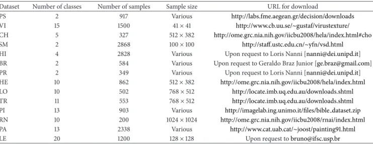
Table 1: Descriptive summary of the image datasets.

Dataset Number of classes Number of samples Sample size URL for download

PS 2 917 Various http://labs.fme.aegean.gr/decision/downloads

VI 15 1500 41×41 http://www.cb.uu.se/∼gustaf/virustexture/

CH 5 327 512×382 http://ome.grc.nia.nih.gov/iicbu2008/hela/index.html#cho

SM 2 2868 100×100 http://staff.ustc.edu.cn/∼yfn/vsd.html

HI 4 2828 Various Upon request to Loris Nanni [[email protected]]

BR 2 584 Various Upon request to Geraldo Braz Junior [[email protected]]

PR 2 349 Various Upon request to Loris Nanni [[email protected]]

HE 10 862 512×382 http://ome.grc.nia.nih.gov/iicbu2008/hela/index.html

LO 10 502 768×512 http://locate.imb.uq.edu.au/downloads.shtml

TR 11 553 768×512 http://locate.imb.uq.edu.au/downloads.shtml

PI 13 903 Various http://imagelab.ing.unimo.it/files/bible dataset.zip

RN 10 200 1024×1024 http://ome.grc.nia.nih.gov/iicbu2008/rnai/index.html

PA 13 2338 Various http://www.cat.uab.cat/∼joost/painting91.html

LE 20 1200 128×128 Upon request [email protected]

(iii) CH: this dataset, reported in [28], contains fluores-cent microscopy images taken from Chinese hamster ovary cells that belong to five different classes. (iv) SM: this dataset, reported in [29], contains images

extracted from video-based smoke detection surveil-lance systems. The same division of the dataset into training/testing sets, reported in [29], is used in this paper.

(v) HI: this dataset, reported in [30], contains images extracted from four fundamental tissues.

(vi) BR: this dataset, reported in [31], contains 273 malig-nant and 311 benign breast cancer images.

(vii) PR: this is a dataset containing 118 DNA-binding proteins and 231 non-DNA-binding proteins. Texture descriptors are extracted from the 2D distance matrix that represents each protein. This matrix is obtained from the 3D tertiary structure of a given protein considering only atoms that belong to the protein backbone (see [32] for details).

(viii) HE: the 2D HeLa dataset [28] contains single cell images divided into 10 staining classes that were taken from fluorescence microscope acquisitions on HeLa cells.

(ix) LO: the locate endogenous mouse subcellular organelles dataset [33] contains 502 images unevenly distributed among 10 classes of endogenous proteins or features of specific organelles.

(x) TR: the locate transfected mouse subcellular organelles dataset [33] contains 553 images unevenly distributed in 11 classes of fluorescence-tagged or epitope-tagged proteins transiently expressed in specific organelles.

(xi) PI: this dataset, reported in [34], contains pictures extracted from digitalized pages of the Holy Bible of Borso d’Este, duke of Ferrara, Italy, from 1450 AD to 1471 AD. PI is composed of 13 classes, characterized

by a clear semantic meaning and significant search relevance.

(xii) RN: this is a dataset containing 200 fluorescence microscopy images evenly distributed among 10 classes of fly cells subjected to a set of gene knock-downs using RNAi. The cells were stained with DAPI to visualize their nuclei.

(xiii) PA: this dataset, reported in [35], contains 2338 paintings by 50 painters, representative of 13 different painting styles: abstract expressionism, baroque, con-structivism, cubism, impressionism, neoclassical, pop art, postimpressionism, realism, renaissance, roman-ticism, surrealism, and symbolism. A split train-ing/testing set is provided by the authors [35] and is used in this paper.

(xiv) LE: this dataset contains images of 20 species of Brazilian flora [36]. A total of 400 samples, divided into 20 classes (20 samples per class), were collected. Three windows were extracted from each sample. A constraint to the fivefold cross-validation technique was added that required that all windows extracted from a given leaf belong either to the training set or to the testing set, not both.

A descriptive summary of each dataset, along with the URL where each dataset can be downloaded, is reported in Table1. If a dataset contains RGB images, these were con-verted to grey-level images before the feature extraction step. The testing protocol used with these datasets is the fivefold cross-validation method, with the exception of three dataset, SM, VI, and PA, where the protocols and testing/training sets defined by the datasets were used (these protocols, which are briefly described above, were obtained from the creators of each of these datasets).

4.2. UCI Data Mining Datasets. We report results obtained using eleven datasets from the UCI repository [37]. In Table2 we list each dataset used in this study and describe each

(7)

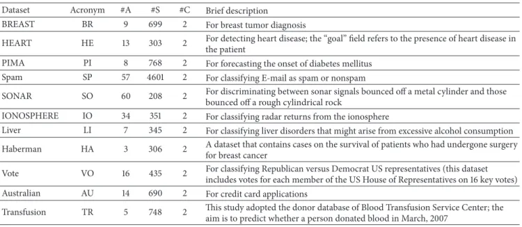
Table 2: UCI datasets and their features: number of attributes (#A), number of samples (#S), and number of classes (#C).

Dataset Acronym #A #S #C Brief description

BREAST BR 9 699 2 For breast tumor diagnosis

HEART HE 13 303 2 For detecting heart disease; the “goal” field refers to the presence of heart disease in

the patient

PIMA PI 8 768 2 For forecasting the onset of diabetes mellitus

Spam SP 57 4601 2 For classifying E-mail as spam or nonspam

SONAR SO 60 208 2 For discriminating between sonar signals bounced off a metal cylinder and those

bounced off a rough cylindrical rock

IONOSPHERE IO 34 351 2 For classifying radar returns from the ionosphere

Liver LI 7 345 2 For classifying liver disorders that might arise from excessive alcohol consumption

Haberman HA 3 306 2 A dataset that contains cases on the survival of patients who had undergone surgery

for breast cancer

Vote VO 16 435 2 For classifying Republican versus Democrat US representatives (this dataset

includes votes for each member of the US House of Representatives on 16 key votes)

Australian AU 14 690 2 For credit card applications

Transfusion TR 5 748 2 This study adopted the donor database of Blood Transfusion Service Center; the

aim is to predict whether a person donated blood in March, 2007

of them according to the number of attributes (#A), the number of samples (#S), and the number of classes (#C) that each contains. The testing protocol is the fivefold cross-validation method. All features in these datasets were linearly normalized between 0 and 1 before classification, using only the training data for normalizing the test data. In all the tests the testing set is completely blind.

5. Results and Discussion

The performance indicator used in all experiments is the area under the ROC curve (AUC) because it provides a better overview of classification results [38]. In the multi-class problem, AUC is calculated using the one-versus-all approach, where a given class is considered “positive” and all other classes are considered “negative.” The average AUC is reported in all tables.

In order to better compare the ensembles, we also con-sider their average AUC (Av) and the average rank (RA) obtained in all datasets. RA should be minimized: if a classifier obtains the perfect classification in all the datasets, its RA is 1. The last row labelled Av in all the tables included in this section reports the average AUC performance on all the datasets. To statistically validate these experiments, the Wilcoxon Signed-Rank test [39] was used for all methods.

For the purpose of reproducing and comparing results, the split training/testing sets used for each dataset are available at the website listed at the end of the Introduction. For the image datasets, we also provide both the LTP and LPQ features that were extracted from each dataset for this study.

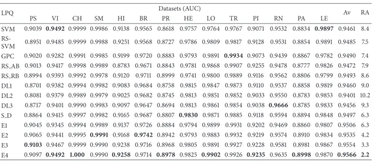
5.1. Experimental Results in Image Classification. The first set of experiments are aimed at comparing the performance of the proposed approaches with the stand-alone methods described in Section 2. Tables 3 and 4 report the results obtained by the state-of-the-art classifiers, trained with LTP

and LPQ, respectively, and the following heterogeneous ensembles based on the sum rule:

(i) S D: (DL1 + DL2 + DL3)/3. (ii) E1: GPC + RS AB.

(iii) E2: GPC + RS AB + RS RB.

(iv) E3: GPC + RS AB + RS RB + RS-SVM. (v) E4: GPC + RS AB + RS RB + RS-SVM + S D. A + B is the sum rule applied to classifier A and classifier B, after classifier scores have been normalized to mean 0 and standard deviation 1.

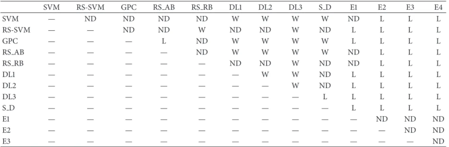
In Table5, we compare the classifier performances given in Tables3and4using the Wilcoxon Signed-Rank test. Three symbols are used in Table5:

(i) “𝐿” indicates that the method in the given row exhibits a lower performance (with 𝑝value <0.10) than the method listed in the corresponding column (i.e., the classifier in that row is the “loser” compared with the column classifier).

(ii) “ND” indicates that there is no statistically significant difference between the performances of the two meth-ods.

(iii) “𝑊” indicates that the method in the given row exhibits a higher performance, with𝑝value <0.10, than the method listed in the corresponding column (i.e., the classifier in that row is the “winner” com-pared with the column classifier).

Analyzing the results reported in Table 5, we observe some very interesting results:

(i) Both SVM and RS-SVM fail to outperform any of the other state-of-the-art approaches.

(8)

Table 3: Performance (AUC) obtained in different image datasets using LTP as texture descriptor. LTP Datasets (AUC) Av RA PS VI CH SM HI BR PR HE LO TR PI RN PA LE SVM 0.9144 0.9349 1.000 0.9975 0.9156 0.9692 0.8968 0.9814 0.9949 0.9926 0.9286 0.9696 0.8903 0.9792 0.9546 7.0 RS-SVM 0.9071 0.9352 1.000 0.9976 0.9195 0.9763 0.9030 0.9826 0.9950 0.9924 0.9316 0.9713 0.8944 0.9807 0.9562 5.9 GPC 0.9086 0.9131 0.9997 0.9971 0.9198 0.9789 0.8865 0.9816 0.9964 0.9930 0.9090 0.9769 0.8968 0.9752 0.9523 8.1 RS AB 0.9121 0.9254 0.9998 0.9974 0.8924 0.9810 0.9079 0.9813 0.9965 0.9953 0.9242 0.9771 0.8959 0.9738 0.9543 7.0 RS RB 0.9110 0.9293 0.9999 0.9953 0.9136 0.9739 0.8886 0.9806 0.9969 0.9955 0.9178 0.9900 0.8940 0.9738 0.9543 7.6 DL1 0.8927 0.9173 0.9999 0.9952 0.9072 0.9811 0.8486 0.9801 0.9962 0.9965 0.9147 0.9837 0.8865 0.9811 0.9486 8.7 DL2 0.8965 0.9220 0.9998 0.9956 0.8945 0.9815 0.8780 0.9806 0.9956 0.9959 0.9061 0.9878 0.8869 0.7900 0.9365 9.4 DL3 0.7802 0.9239 0.9999 0.9963 0.9082 0.9815 0.8779 0.9812 0.9958 0.9962 0.9014 0.9916 0.8895 0.9525 0.9412 8.5 S D 0.8985 0.9244 1.000 0.9958 0.9143 0.9835 0.8783 0.9818 0.9958 0.9966 0.9151 0.9916 0.8960 0.9806 0.9537 6.0 E1 0.9130 0.9196 0.9997 0.9974 0.9162 0.9812 0.8999 0.9816 0.9962 0.9945 0.9191 0.9798 0.8983 0.9748 0.9551 7.2 E2 0.9165 0.9337 0.9998 0.9973 0.9184 0.9809 0.9007 0.9837 0.9969 0.9960 0.9238 0.9884 0.9030 0.9768 0.9583 5.1 E3 0.9165 0.9361 1.000 0.9975 0.9229 0.9816 0.9090 0.9843 0.9970 0.9968 0.9313 0.9835 0.9080 0.9796 0.9603 2.8 E4 0.9164 0.9372 1.000 0.9975 0.9235 0.9824 0.9059 0.9851 0.9973 0.9971 0.9318 0.9864 0.9093 0.9808 0.9608 2.2

Table 4: Performance obtained on the different image datasets using LPQ as texture descriptor.

LPQ Datasets (AUC) Av RA PS VI CH SM HI BR PR HE LO TR PI RN PA LE SVM 0.9039 0.9492 0.9999 0.9986 0.9138 0.9565 0.8618 0.9757 0.9764 0.9767 0.9071 0.9532 0.8834 0.9897 0.9461 8.4 RS-SVM 0.8951 0.9485 0.9999 0.9988 0.9251 0.9568 0.8727 0.9786 0.9809 0.9817 0.9128 0.9531 0.8854 0.9891 0.9485 7.5 GPC 0.9020 0.9282 0.9991 0.9985 0.9199 0.9720 0.8883 0.9793 0.9891 0.9934 0.9073 0.9439 0.8867 0.9782 0.9490 7.4 RS AB 0.9013 0.9417 0.9998 0.9989 0.8783 0.9671 0.8843 0.9781 0.9868 0.9907 0.9255 0.9478 0.8777 0.9826 0.9472 7.9 RS RB 0.8994 0.9393 0.9992 0.9978 0.9120 0.9711 0.8999 0.9741 0.9800 0.9889 0.9116 0.9562 0.8806 0.9799 0.9493 8.6 DL1 0.8701 0.9382 0.9994 0.9982 0.9083 0.9684 0.8758 0.9815 0.9847 0.9873 0.9110 0.9537 0.8858 0.9819 0.9460 9.0 DL2 0.8081 0.9379 0.9989 0.9979 0.9025 0.9682 0.8745 0.9813 0.9851 0.9852 0.9033 0.9550 0.8783 0.9853 0.9401 10.2 DL3 0.8717 0.9401 0.9990 0.9983 0.9097 0.9647 0.8694 0.9813 0.9861 0.9854 0.9038 0.9666 0.8785 0.9833 0.9456 9.3 S D 0.8864 0.9415 0.9997 0.9982 0.9165 0.9687 0.8807 0.9830 0.9871 0.9885 0.9118 0.9594 0.8894 0.9848 0.9497 6.3 E1 0.9045 0.9345 0.9994 0.9989 0.9137 0.9726 0.8884 0.9794 0.9899 0.9931 0.9202 0.9469 0.8860 0.9807 0.9506 6.3 E2 0.9065 0.9441 0.9995 0.9991 0.9168 0.9742 0.8942 0.9793 0.9883 0.9932 0.9219 0.9574 0.8910 0.9834 0.9535 4.2 E3 0.9103 0.9467 0.9999 0.9990 0.9238 0.9716 0.8968 0.9805 0.9891 0.9927 0.9228 0.9581 0.8981 0.9867 0.9554 3.3 E4 0.9097 0.9492 1.000 0.9990 0.9258 0.9714 0.8978 0.9825 0.9902 0.9926 0.9235 0.9635 0.8998 0.9870 0.9566 2.2

Table 5: Comparisons between all the pairs of tested methods.

SVM RS-SVM GPC RS AB RS RB DL1 DL2 DL3 S D E1 E2 E3 E4 SVM — L ND L ND ND ND ND ND L L L L RS-SVM — — ND L ND ND ND ND ND L L L L GPC — — — ND ND ND W W ND L L L L RS AB — — — — ND W W W ND ND L L L RS RB — — — — — W W ND ND L L L L DL1 — — — — — — ND ND L L L L L DL2 — — — — — — — ND L L L L L DL3 — — — — — — — — ND L L L L S D — — — — — — — — — ND L L L E1 — — — — — — — — — — L L L E2 — — — — — — — — — — — L L E3 — — — — — — — — — — — — L

(9)

Table 6: Performance on the different data mining datasets. Datasets (AUC) Av RA BR HE PI SP SO IO LI HA VO AU TR SVM 0.9941 0.8809 0.824 0.9708 0.9517 0.9814 0.7558 0.7012 0.9855 0.9164 0.714 0.8796 7.3077 RS-SVM 0.9931 0.9076 0.8221 0.9771 0.9591 0.9795 0.7411 0.6399 0.9853 0.9221 0.6931 0.8745 8.6923 GPC 0.9924 0.9024 0.827 0.979 0.9409 0.9713 0.729 0.6804 0.9882 0.9267 0.7295 0.8788 8.000 RS AB 0.991 0.9101 0.8229 0.988 0.9371 0.9788 0.7581 0.6727 0.9887 0.9313 0.735 0.8831 7.000 RS RB 0.9925 0.9169 0.8208 0.9873 0.9334 0.9851 0.7664 0.6071 0.9884 0.9326 0.674 0.8731 7.3846 DL1 0.9943 0.8852 0.8252 0.966 0.8794 0.9222 0.7541 0.6751 0.9795 0.9155 0.7338 0.8664 8.7692 DL2 0.9941 0.8754 0.8149 0.9691 0.8789 0.9242 0.7478 0.6679 0.9808 0.9088 0.7318 0.8631 10.3077 DL3 0.9943 0.8941 0.8193 0.9684 0.8501 0.9022 0.6966 0.6537 0.9787 0.9154 0.7351 0.8553 10.2308 S D 0.9942 0.883 0.8238 0.9683 0.8781 0.9297 0.751 0.6772 0.9813 0.9186 0.7357 0.8674 8.6154 E1 0.992 0.9096 0.8277 0.9856 0.9426 0.9772 0.7532 0.6868 0.9896 0.9331 0.7372 0.885 6.000 E2 0.9924 0.9124 0.8285 0.988 0.9426 0.9817 0.7727 0.6724 0.9897 0.935 0.7257 0.8856 5.3846 E3 0.9933 0.9141 0.8288 0.9873 0.9508 0.9819 0.7723 0.6726 0.989 0.9343 0.7258 0.8864 5.0769 E4 0.9934 0.9113 0.8294 0.9862 0.942 0.9805 0.7717 0.6794 0.9895 0.9339 0.7297 0.8861 5.2308

Table 7: Comparisons between all the pairs of methods tested in Table6.

SVM RS-SVM GPC RS AB RS RB DL1 DL2 DL3 S D E1 E2 E3 E4 SVM — ND ND ND ND W W W W ND L L L RS-SVM — — ND ND W ND ND W ND L L L L GPC — — — L ND W W W W L L L L RS AB — — — — ND W W W W ND L L L RS RB — — — — — ND ND W ND ND L L L DL1 — — — — — — W W ND L L L L DL2 — — — — — — — W ND L L L L DL3 — — — — — — — — L L L L L S D — — — — — — — — — L L L L E1 — — — — — — — — — — ND ND ND E2 — — — — — — — — — — — ND ND E3 — — — — — — — — — — — — ND

(iii) E4 (the fusion among all the base methods) always obtains the highest performance.

(iv) The simple ensemble S D obtains a performance that is comparable with all the other base methods. (v) RS, which involved no parameter tuning step,

outper-forms SVM (implemented with LibSVM) where the parameters are optimally tuned for each dataset.

5.2. Experiments Results in Data Mining Datasets. The same tests reported in the previous section using the image datasets are also run for the data mining datasets. The results reported in Tables6and7clearly show the usefulness of our ensemble approach.

In these tests we obtain results that are similar to those reported in Tables3and4, but there is an important differ-ence: RS-SVM works poorly in the two datasets containing few features (HA and TR). The reason for this is simple: when only a few features are used to describe a pattern, they are likely to be uncorrelated, so an RS approach is not

advised. When the datasets HA and TR are removed from consideration, RS-SVM outperforms SVM. Notice as well that in this test the ensembles outperform the base methods.

6. Conclusions

The aim of this paper was to compare and combine several state-of-the-art classifiers for proposing a GP ensemble that works well across a broad set of datasets (fourteen different image datasets and eleven UCI data mining datasets) with no parameter tuning. No single approach was discovered that outperformed all the other classifier systems in all the tested datasets. This finding lends support to the “no free lunch” hypothesis/metaphor that claims that “any two algorithms are equivalent when their performance is averaged across all possible problems” [40]. Nonetheless, several interesting findings are obtained when examining the classifier results across the twenty-five datasets:

(i) Among the different state-of-the-art methods, there is no winner.

(10)

(ii) The GP ensembles clearly outperform the state-of-the-art methods without any complex fusion rule (the simple sum rule is used throughout the exper-iments). In particular, the GP ensembles outper-form SVM implemented with the LibSVM toolbox, which is probably the most used classification toolbox reported in the literature.

In our opinion, a heterogeneous system based on different state-of-the-art classifiers (including classifiers that are them-selves an ensemble, such as a random subspace of rotation boosting) is the most feasible way of avoiding the “curse” of the “no free lunch” metaphor.

There are many avenues for exploring GP ensembles fur-ther. A suggested list of future explorations is the following:

(i) Test the performance of ensembles using more com-plex fusion rules.

(ii) Test systems on data mining problems where a large set of features is available.

(iii) Expand the base methods to combine different deep learning approaches, such as an extreme learning machine [41] or convolutional neural networks [42] where the input is the whole image and not a feature vector.

Conflict of Interests

The authors declare that there is no conflict of interests regarding the publication of this paper.

References

[1] L. I. Kuncheva and C. J. Whitaker, “Measures of diversity in classifier ensembles and their relationship with the ensemble

accuracy,”Machine Learning, vol. 51, no. 2, pp. 181–207, 2003.

[2] J. Kittler, M. Hatef, R. P. W. Duin, and J. Matas, “On combining

classifiers,”IEEE Transactions on Pattern Analysis and Machine

Intelligence, vol. 20, no. 3, pp. 226–239, 1998.

[3] L. Breiman, “Arcing classifiers,”The Annals of Statistics, vol. 26,

no. 3, pp. 801–849, 1998.

[4] G. Bologna and R. D. Appel, “A comparison study on protein

fold recognition,” inProceedings of the 9th International

Confer-ence on Neural Information Processing (ICONIP ’02), vol. 5, pp. 2492–2496, IEEE, Singapore, November 2002.

[5] G. Mart´ınez-Mu˜noz and A. Su´arez, “Switching class labels to

generate classification ensembles,”Pattern Recognition, vol. 38,

no. 10, pp. 1483–1494, 2005.

[6] P. Melville and R. J. Mooney, “Creating diversity in ensembles

using artificial data,”Information Fusion, vol. 6, no. 1, pp. 99–

111, 2005.

[7] T. K. Ho, “The random subspace method for constructing

decision forests,”IEEE Transactions on Pattern Analysis and

Machine Intelligence, vol. 20, no. 8, pp. 832–844, 1998.

[8] K. Tumer and N. C. Oza, “Input decimated ensembles,”Pattern

Analysis and Applications, vol. 6, no. 1, pp. 65–77, 2003. [9] L. Nanni and A. Lumini, “Ensemble generation and feature

selection for the identification of students with learning

disabil-ities,”Expert Systems with Applications, vol. 36, no. 2, pp. 3896–

3900, 2009.

[10] L. Breiman, “Random forests,”Machine Learning, vol. 45, no. 1,

pp. 5–32, 2001.

[11] S. Kotsiantis and V. Tampakas, “Combining heterogeneous

clas-sifiers: a recent overview,”Journal of Convergence Information

Technology, vol. 6, no. 10, pp. 164–172, 2011.

[12] L. Nanni, S. Brahnam, and A. Lumini, “Double committee

adaboost,”Journal of King Saud University—Science, vol. 25, no.

1, pp. 29–37, 2013.

[13] L. Nanni, A. Lumini, and S. Brahnam, “An empirical study of

different approaches for protein classification,”The Scientific

World Journal, vol. 2014, Article ID 236717, 17 pages, 2014. [14] X. Tan and B. Triggs, “Enhanced local texture feature sets for

face recognition under difficult lighting conditions,” inAnalysis

and Modelling of Faces and Gestures, vol. 4778 ofLecture Notes in Computer Science, pp. 168–182, Springer, 2007.

[15] V. Ojansivu and J. Heikkila, “Blur insensitive texture

classifica-tion using local phase quantizaclassifica-tion,” inProceedings of the 3rd

International Conference on Image and Signal Processing (ICISP

’08), pp. 236–243, 2008.

[16] N. Cristianini and J. Shawe-Taylor,An Introduction to Support

Vector Machines and Other Kernel-Based Learning Methods, Cambridge University Press, Cambridge, UK, 2000.

[17] C. E. Rasmussen and C. K. Williams, Gaussian Processes

for Machine Learning, Adaptive Computation and Machine Learning, The MIT Press, 2006.

[18] Y. Freund and R. E. Schapire, “A short introduction to boosting,”

Journal of Japanese Society for Artificial Intelligence, vol. 14, no. 5, pp. 771–780, 1999.

[19] C.-X. Zhang and J.-S. Zhang, “RotBoost: a technique for

combining Rotation Forest and AdaBoost,”Pattern Recognition

Letters, vol. 29, no. 10, pp. 1524–1536, 2008.

[20] G. E. Hinton, S. Osindero, and Y.-W. Teh, “A fast learning

algorithm for deep belief nets,”Neural Computation, vol. 18, no.

7, pp. 1527–1554, 2006.

[21] R. Socher, B. Huval, B. Bhat, C. D. Manning, and A. Y. Ng, “Convolutional-recursive deep learning for 3D object

classifica-tion,” inAdvances in Neural Information Processing Systems 25,

F. Pereira, C. J. C. Burges, L. Bottou, and K. Q. Weinberger, Eds., pp. 1–9, 2012.

[22] Y. Sun, X. Wang, and X. Tang, “Hybrid deep learning for face

verification,” inProceedings of the IEEE International Conference

on Computer Vision (ICCV ’13), pp. 1489–1496, IEEE, Sydney, Australia, December 2013.

[23] K. Hornik, M. Stinchcombe, and H. White, “Multilayer

feedfor-ward networks are universal approximators,”Neural Networks,

vol. 2, no. 5, pp. 359–366, 1989.

[24] T. Ojala, M. Pietikäinen, and T. Mäenpää, “Multiresolution gray-scale and rotation invariant texture classification with local

binary patterns,” IEEE Transactions on Pattern Analysis and

Machine Intelligence, vol. 24, no. 7, pp. 971–987, 2002.

[25] X. He, D. Cai, S. Yan, and H.-J. Zhang, “Neighborhood

preserv-ing embeddpreserv-ing,” inProceedings of the 10th IEEE International

Conference on Computer Vision (ICCV ’05), Beijing, China, October 2005.

[26] J. Jantzen, G. Dounias, and B. Bjerregaard, “Pap-smear

bench-mark data for pattern classification,” in Proceedings of the

European Symposium on Nature Inspired Smart Information Systems (NiSIS ’05), pp. 1–9, Albufeira, Portugal, 2005. [27] G. Kylberg, M. Uppstr¨om, K.-O. Hedlund, G. Borgefors, and

I.-M. Sintorn, “Segmentation of virus particle candidates in

trans-mission electron microscopy images,”Journal of Microscopy,

(11)

[28] M. V. Boland and R. F. Murphy, “A neural network classifier capable of recognizing the patterns of all major subcellular structures in fluorescence microscope images of HeLa cells,”

Bioinformatics, vol. 17, no. 12, pp. 1213–1223, 2002.

[29] F. Yuan, “Video-based smoke detection with histogram

sequence of LBP and LBPV pyramids,”Fire Safety Journal, vol.

46, no. 3, pp. 132–139, 2011.

[30] A. Cruz-Roa, J. C. Caicedo, and F. A. Gonz´alez, “Visual pattern mining in histology image collections using bag of features,”

Artificial Intelligence in Medicine, vol. 52, no. 2, pp. 91–106, 2011. [31] G. B. Junior, A. C. de Paiva, A. C. Silva, and A. C. M. de Oliveira, “Classification of breast tissues using Moran’s index and Geary’s

coefficient as texture signatures and SVM,”Computers in Biology

and Medicine, vol. 39, no. 12, pp. 1063–1072, 2009.

[32] L. Nanni, J.-Y. Shi, S. Brahnam, and A. Lumini, “Protein clas-sification using texture descriptors extracted from the protein

backbone image,”Journal of Theoretical Biology, vol. 264, no. 3,

pp. 1024–1032, 2010.

[33] N. A. Hamilton, R. S. Pantelic, K. Hanson, and R. D. Teasdale,

“Fast automated cell phenotype image classification,” BMC

Bioinformatics, vol. 8, article 110, 2007.

[34] D. Borghesani, C. Grana, and R. Cucchiara, “Miniature illustra-tions retrieval and innovative interaction for digital illuminated

manuscripts,”Multimedia Systems, vol. 20, no. 1, pp. 65–79, 2014.

[35] F. S. Khan, S. Beigpour, J. van de Weijer, and M. Felsberg, “Painting-91: a large scale database for computational painting

categorization,”Machine Vision and Applications, vol. 25, no. 6,

pp. 1385–1397, 2014.

[36] D. Casanova, J. J. de Mesquita, and O. M. Bruno, “Plant leaf

identification using gabor wavelets,”International Journal of

Imaging Systems and Technology, vol. 19, no. 3, pp. 236–243, 2009.

[37] A. Frank and A. Asuncion, UCI Machine Learning Repository, 2010.

[38] T. Fawcett,ROC Graphs: Notes and Practical Considerations for

Researchers, HP Laboratories, Palo Alto, Calif, USA, 2004. [39] J. Demˇsar, “Statistical comparisons of classifiers over multiple

data sets,”Journal of Machine Learning Research, vol. 7, pp. 1–30,

2006.

[40] D. H. Wolpert and W. G. Macready, “Coevolutionary free

lunches,”IEEE Transactions on Evolutionary Computation, vol.

9, no. 6, pp. 721–735, 2005.

[41] G.-B. Huang, X. Ding, and H. Zhou, “Optimization method

based extreme learning machine for classification,”

Neurocom-puting, vol. 74, no. 1–3, pp. 155–163, 2010.

[42] R. B. Palm,Prediction as a candidate for learning deep

hierar-chical models of data [M.S. thesis], DTU Informatics, Technical Univeristy of Denmark, Kongens Lyngby, Denmark, 2012.

(12)

Submit your manuscripts at

http://www.hindawi.com

Computer Games Technology International Journal of

Hindawi Publishing Corporation

http://www.hindawi.com Volume 2014

http://www.hindawi.com Volume 2014 Distributed Sensor Networks International Journal of Advances in

Fuzzy

Systems

International Journal of

Reconfigurable Computing

Applied

Computational

Intelligence and Soft

Computing

Advances in

Artificial

Intelligence

Hindawi Publishing Corporation http://www.hindawi.com Volume 2014 Advances in Software Engineering

Electrical and Computer Engineering

Journal of Journal of

Computer Networks and Communications

Hindawi Publishing Corporation

http://www.hindawi.com Volume 2014

Multimedia

International Journal of

Biomedical Imaging

Artificial

Neural Systems

Advances in

Robotics

Journal of

http://www.hindawi.com Volume 2014 Hindawi Publishing Corporationhttp://www.hindawi.com Volume 2014

Computational Intelligence and Neuroscience

Modelling & Simulation in Engineering

The Scientific

World Journal

http://www.hindawi.com Volume 2014 Human-Computer Interaction

Advances in

Computer EngineeringAdvances in Hindawi Publishing Corporation