Weierstraß-Institut
f¨
ur Angewandte Analysis und Stochastik
im Forschungsverbund Berlin e.V.
Preprint
ISSN 0946 – 8633
Spetral estimation of the frational order
of a Lévy proess
Denis Belomestny
submitted: Marh 20,2010
WeierstrassInstitute
forAppliedAnalysisandStohastis Mohrenstr. 39 10117Berlin Germany E-Mail: Denis.Belomestnywias-berlin.de No. 1491 Berlin2010
2000Mathematics Subject Classification. 62F10, 62J12, 62F25, 62H12..
Key words and phrases. Regular Levy processes, Blumenthal-Getoor index, semiparametric estima-tion.
Weierstraÿ-Institutfür Angewandte Analysis und Stohastik (WIAS) Mohrenstraÿe 39 10117 Berlin Germany Fax: +49 302044975 E-Mail: preprintwias-berlin.de World WideWeb: http://www.wias-berlin.de/
Abstract
We consider the problem of estimating the fractional order of a L´evy process from low frequency historical and options data. An estimation methodology is developed which allows us to treat both estimation and calibration problems in a unified way. The corresponding procedure consists of two steps: the estimation of a conditional characteristic function and the weighted least squares estimation of the fractional order in spectral domain. While the second step is identical for both calibration and estimation, the first one depends on the problem at hand. Minimax rates of convergence for the fractional order estimate are derived, the asymptotic normality is proved and a data-driven algorithm based on aggregation is proposed. The performance of the estimator in both estimation and calibration setups is illustrated by a simulation study.
1
Introduction
Nowadays L´evy processes are undoubtedly one of the most popular tool for modeling eco-nomic and financial time series (see e.g. Cont and Tankov, 2004, for an overview). This is not surprising if one takes into account their simplicity and analytic tractability on the one hand and the ability to reproduce many stylized facts of financial time series on the other hand. In the last decade, new subclasses of L´evy processes have been introduced and actively studied (mainly in the context of option pricing). Among the best known models are normal inverse Gaussian processes (NIG), hyperbolic processes (HP), gener-alized hyperbolic processes (GHP) and truncated (or tempered) L´evy processes (TLP). Boyarchenko and Levendorski˘ı (2002) have introduced a general class of regular L´evy processes of exponential type (RLE) which contains all above mentioned particular L´evy models. This type of processes is characterized by the requirement that the modulus of the characteristic function of increments behaves like exp(−η|u|α) as |u| → ∞ for some
0< α <2. Parameterαcoincides with the fractional order of the underlying L´evy process and plays an important role because it determines the decay of the characteristic function and hence the smoothness properties of the corresponding state price density. Statistical inference for RLE processes is the subject of our paper.
There are basically two types of statistical problems relevant for L´evy processes: the estimation of parameters of a L´evy processXtfrom a time series of the assetSt= exp(Xt)
and the calibration of these parameters using options data. Both problems have got much attention recently.
Suppose that a L´evy processXtis observed atntime points ∆,2∆, . . . , n∆.SinceX0 = 0,
this amounts to observing n increments χi = Xi∆−X(i−1)∆, i = 1, . . . , n. If ∆ is small
(high-frequency data), then a large increment χi indicates that a jump occurred between
time ti−1 and ti. Based on this insight and the continuous-time observation analogue,
inference for the L´evy measure of the underlying L´evy process can be conducted. See, for example, A¨ıt-Sahalia and Jacod (2006) for a semiparametric problem of estimating
volatility of a stable process under the presence of L´evy perturbation or Lee and Mykland (2007) and Figueroa-L´opez and Houdr´e (2006) for a nonparametric problems of testing and estimation for jump diffusion models. For low-frequency observations, however, we cannot be sure to what extent the increment χi is due to one or several jumps or just
to the diffusion part of the L´evy process. The only way to draw inference is to use the fact that the increments form independent realizations of infinitely divisible probability distributions. In this setting, a variety of methods have been proposed in the literature: standard maximum likelihood estimation (DuMouchel, 1973a,b, 1975), using the empiri-cal characteristic function as an estimating equation (see e.g. Press, 1972; Fenech, 1976; Feuerverger and McDunnough, 1981a; Singleton, 2001), maximum likelihood by Fourier inversion of the characteristic function (Feuerverger and McDunnough, 1981b), a regres-sion based on the explicit form of the characteristic function (Koutrouvelis, 1980), or other numerical approximations (Nolan, 1997). Some of these methods were compared in Akgiray and Lamoureux (1989). Note that all of the aforementioned papers deal with the specific parametric (mainly stable) models. A semiparametric estimation problem for L´evy models has recently been considered in Neumann and Reiß (2007) and Gugushvili (2008).
The second, calibration problem is of special importance for financial applications because pricing of options is performed under an equivalent martingale measure and one can infer on this measure only from options data. Since option data is sparse and the underly-ing inverse problem is usually ill-posed, we face a rather complicated estimation issue. Different approaches have been proposed in the literature to regularize the underlying inverse problem. For example, in Cont and Tankov (2004) and Cont and Tankov (2006) a method based on the penalized least squares estimation with the minimal entropy penal-ization is proposed. Belomestny and Reiß (2006) developed a spectral calibration method which avoids solving a high dimensional optimization problem and is based on the direct inversion of a Fourier pricing formula with a cut-off regularization in spectral domain. This method essentially employees the integrability property of the underlying L´evy mea-sure (finite activity L´evy processes) that excludes many interesting infinite activity L´evy processes.
In this paper we consider the problem of estimating the fractional order of a L´evy process from low-frequency historical as well as options data. Our problem is semiparametric one because we do not assume any specific parametric model for the underlying process but only some asymptotic behavior. The spectral approach allows us to treat both estimation and calibration problems in a unified framework and leads to an efficient data-driven algorithm. Moreover, the fractional order estimate delivered by the spectral method possesses several interesting optimality properties.
The problem of estimating the degree of activity of jumps in semimartingale framework using high-frequency financial data has recently been considered in A¨ıt-Sahalia and Jacod (2009). On the one hand, small increments of the process turn out to be most informative for estimating the activity index. On the other hand, these small increments are the ones where the contribution from the continuous martingale part is mixed with the contribution from the small jumps. A¨ıt-Sahalia and Jacod (2009) proposed an estimation procedure which is able to “see through” the continuous part and consistently estimate the degree of activity for the small jumps under some restrictions on the structure of the underlying semimartingale. Note that in the case of L´evy processes the degree of activity of jumps is identical to the fractional order of the underlying L´evy process. We also stress that the case when both diffusion and jump components are presented can be treated in the
framework of spectral estimation as well (see Section 6.9).
Short outline of the paper. In Section 2 we introduce the class of RLE processes. Section 3 discusses some aspects of financial modeling with RLE processes. Section 4 describes the observational model. In Section 5 methods of estimating the characteristic function of a L´evy process from low-frequency historical and options data are presented. Section 6 is devoted to the spectral calibration method of estimating the fractional order α. We discuss here the problems of regularization and derive minimax rates of convergence for a class of L´evy processes. In Section 7 adaptive procedure for estimating α is presented and its properties are discussed. We conclude with some simulation results.
2
Regular L´
evy processes of exponential type
In this section we recall some basic properties of L´evy processes.
2.1
Spectral properties of L´
evy processes
Consider a L´evy processXtwith a L´evy measureν. That is,Xt is c`adl`ag process with
in-dependent and stationary increments such that the characteristic function of its marginals φt(u) is given by (2.1) φt(u) := E eiuXt = exp t iuµ− u 2a2 2 + Z R (eiux−1−iux1{|x|≤1})ν(dx) .
So, any L´evy processXtis characterized by the so called L´evy triple (µ, a, ν), whereµ∈R
is a drift, a > 0 is a diffusion volatility and ν is a L´evy measure. Note that the drift µ depends on the type of truncation in (2.1). In fact, this characterization is unique for a fixed truncation function and we can reconstruct L´evy triple from the characteristic function φt(u). This reconstruction may be viewed as consisting of three steps. First,
because of 1 |u|2 Z R (eiux−1−iux1{|x|≤1})ν(dx)→0, |u| → ∞, (2.2)
we can find a2/2 as lim
|u|→∞|u|−2ψ(u) with
ψ(u) =t−1log(φt(u)).
Second, note that Z
1 −1 ( ˜ψ(u)−ψ(u˜ +w))dw= Z R eiuxρ(dx) with ˜ ψ(u) = ψ(u) + a 2 2 u 2, ρ(dx) = 2 1− sinx x ν(dx).
Since ρ is a finite measure (R(x2 ∧1)ν(dx) < ∞), one can uniquely reconstruct it (and
hence ν) from ˜ψ(u). Finally, we find µ as limu→∞ h
˜
ψ(u)/(iu)i. So, in principle, we can recover all characteristics of the underlying L´evy process (including the fractional order) provided that φt is completely known. If, however, φt is estimated from data we face
an ill-posed estimation problem because a small perturbation in φt may deteriorate its
asymptotic behavior and lead to the violation of (2.2). In this case using a regularization technique (see e.g. Cont and Tankov (2004) or Belomestny and Reiß (2006)), we still can get an asymptotically consistent estimates for the whole triple (µ, a, ν) given a consistent estimate of φt.
Remark 2.1. A consistent estimation of ψ(u) from a time series of Xt is only possible
if the number of observations from the distribution with the c. f. φt(u) for some t > 0
increases. This can be either due to a decreasing time step in a times series of the process X (high frequency data) or due to an increasing time horizon (low frequency data). While the first type of observational models has got much attention in recent years, there are only few papers dealing with low frequency data (see e.g. Neumann and Reiß (2007)).
2.2
Fractional order of L´
evy processes
LetXt be a L´evy process with a L´evy measure ν. The value
α := inf r≥0 : Z |x|≤1| x|rν(dx)<∞
is called the fractional order or the Blumenthal-Getoor index of the L´evy process Xt.
This index α is related to the “degree of activity” of jumps. All L´evy measures put finite mass on the set (−∞,−ǫ]∪[ǫ,∞) for any arbitrary ǫ > 0, so if the process has infinite jump activity it must be because of the small “jumps”, defined as those smaller than ǫ. If ν([−ǫ, ǫ]) < ∞ the process has finite activity and α = 0. But if ν([−ǫ, ǫ]) = ∞ i.e. the process has infinite activity and in addition the L´evy measure ν((−∞,−ǫ]∪[ǫ,∞)) diverges near 0 at a rate |ǫ|−α for some α > 0 then the fractional order ofX
t is equal to
α. The higher α gets, the more frequent the small jumps become (see A¨ıt-Sahalia and Jacod (2009) for more discussion).
The Blumenthal-Getoor index is closely related to the notion of the degree of jump activity that applies to general semimartingales as shown in A¨ıt-Sahalia and Jacod (2009), and reduces to the Blumenthal-Getoor index in the special case of L´evy processes.
Note also that the Blumenthal-Getoor index coincides with the stability index for stable processes. Another example of processes having a prescribed fractional orderαis the class of tempered stable processes of order α. Boyarchenko and Levendorski˘ı (2002) studied a generalization of tempered stable processes, called regular L´evy processes of exponential type (RLE). A L´evy process is said to be a RLE process of type [λ−, λ+] and order
α ∈ (0,2) if the L´evy measure has exponentially decaying tails with rates λ− ≥ 0 and
λ+ ≥0 (2.3) Z −1 −∞ eλ−|y|ν(dy)<∞, Z ∞ 1 eλ+yν(dy)<∞
and behaves near zero as |y|−(1+α):
Z |y|>ǫ
ν(dy)≍ Π(ǫ)
ǫα , ǫ→+0,
where Π is some positive function on R+ satisfying 0 < Π(+0) < ∞. Obviously, the fractional order of a RLE process of order α is equal to α. An equivalent definition of a
RLE process in terms of its characteristic exponent ψ(u) can be given as follows. A L´evy process is called to be a RLE process of type [λ−, λ+] and orderα∈(0,2) if the following
representation holds
ψ(u) = iµu+ϑ(u), µ∈R,
(2.4)
where function ϑ admits a continuation from R into the strip {z∈C: Imz ∈[−λ+, λ−]}
and is of the form
ϑ(u) =−|u|απ(u), (2.5)
where π(u) is a function satisfying lim sup|u|→∞|π(u)| < ∞ and lim inf|u|→∞|π(u)| > 0
such that
Re[π(u)]>0, u∈R\ {0}. (2.6)
As was mentioned in the introduction, the class of RLE processes includes among others hyperbolic, normal inverse Gaussian and tempered stable processes but does not include variance Gamma process. In the sequel we will mainly consider RLE processes without regularity conditions (2.3) (or equivalently with λ− = λ+ = 0) since only the behavior
of a L´evy measure near zero matters for the fractional order of the corresponding L´evy process.
As mentioned before, in this work we are going to consider the problem of estimating the fractional order α of a L´evy process Xt from a time series of asset prices as well as from
option prices. Before turning to this, let us first make our modelling and observational framework more precise.
3
Financial modelling
In this section we recall basic facts concerning financial modelling with exponential L´evy models.
3.1
Asset dynamics
We assume that the asset priceStfollows an exponential L´evy model under bothhistorical
measure P and risk neutral measure Q. Specifically, we suppose that St =
(
SeXt, underP, Sert+Yt, underQ,
where Xt and Yt are L´evy processes, S > 0 is the present value of the asset (at time 0)
and r ≥0 is the riskless interest rate which is assumed to be known and constant. Note, that the martingale condition forStunderQentails EQ[eYt] = 1. The martingale measure
Q is in fact not unique under the presence of jumps. As is standard in the calibration literature, it is assumed to be settled by the market and to be identical for all options under consideration. Processes Xt and Yt are related by the requirement that measures
RLE process andXtis of orderαP thenYt has the orderαQ =αP. Indeed, the equivalence
of the corresponding L´evy measures νP and νQ implies (see, Sato (1999))
Z ∞
0
p
dνQ/dνP−12νP(dx)<∞. (3.1)
Since for RLE processes dνQ(x)/dνP(x)
≍x(αP−αQ)
and dνP(x)
≍ x−(1+αP)
dx as x→+0, the condition (3.1) can be satisfied only if αP =αQ. This means that the fractional order of the underlying L´evy process must be the same under both historical and risk-neutral measures. This not only indicates the importance of the fractional order parameter for financial applications but also suggests that the combination of two estimates of the fractional order α under P and Q might be useful e.g. to reduce the overall variance of the resulting combined estimator.
3.2
Option pricing
The risk neutral price at timet= 0 of the European call option with strikeK and maturity T is given by
C(K, T) =e−rTEQ[(S
T −K)+].
Using the independence of increments, we can reduce the number of parameters by intro-ducing the so called negative log-forward moneyness
y:= log(K/S)−rT, such that the call price in terms of y is given by
C(y, T) =SEQ[(eYT −ey)+].
The analogous formula for the price of the European put option is P(y, T) =SEQ[(ey−
eYT)+] and a well-known put-call parity is easily established
C(y, T)−P(y, T) =SEQ[eYT −ey] =S(1−ey). As we need to employ Fourier techniques, we introduce the function
(3.2) OT(y) :=
(
S−1C(y, T), y≥0,
S−1P(y, T), y <0.
The function OT records normalized call prices for y ≥ 0 and normalized put prices for
y < 0. It possesses many interesting properties (see, Belomestny and Reiß (2006) for details) one of them being the following connection between the Fourier transform of OT
and the characteristic function of YT denoted byφQT
(3.3) F[OT](v) =
1−φQT(v−i)
v(v−i) , v ∈R.
Another property which directly follows from (3.3) is that (3.4)
Z
R
e−2yOT(y)dy <∞,
4
Observations
We consider two kinds of observational models corresponding to two types of statistical problems we are going to tackle. While the first type of models assumes the a time series of St is directly available, the second one supposes that only some functionals of St can
be observed.
4.1
Time series data
We assume that the values of the log-price process Xt= log(St) on equidistant time grid
π ={t0, t1, . . . , tn} are observed.
4.2
Option data
As to option data, we assume to be given the prices of n call options for a set of forward log-moneynesses y0 < y1 < . . . < ynand a fixed maturity T, corrupted by noise. In terms
of the function O, the following sample is available
(4.1) OT(yj) =OT(yj) +σ(yj)ξj, j = 1, . . . , n.
It is supposed that {ξj} are independent centered random variables with E[ξj2] = 1 and
supjE[ξ4
j]<∞. Furthermore, we assume that
Z
R
e−2yσ2(y)dy <∞.
This condition is required because we need to transform the original regression model (4.1) to an exponentially weighted one
(4.2) OeT(yj) =OeT(yj) +eσ(yj)ξj, j = 1, . . . , n
with OeT(y) =e−yO
T(y), OeT(y) = e−yOT(y) andeσ(y) =e−yσ(y).
As a matter of fact, a consistent estimation of the fractional order αis only possible if the amount of data available increases. In our asymptotic analysis we will therefore assume that the number of time series observations and the number of available options tend to infinity.
5
Estimation of characteristic functions
φ
Pand
φ
Q The main idea of the spectral estimation method (SEM) is to infer on the parameters of the underlying model using its special structure in the spectral domain. Since spectral behavior of a RLE process is described explicitly by (2.4)-(2.5), we can apply SEM as soon as an estimate for the corresponding characteristic function is available. While estimation of φunderPis rather straightforward, its calibration from option prices underQrequires special treatment.5.1
Estimation of
φ
under
P
We estimate the characteristic function φP
|π|(u) by its empirical counterpart
˜ φP |π|(u) = 1 n n X j=1 eiu(Xtj−Xtj−1).
The empirical characteristic function φ˜P
|π| possesses many interesting properties and we
refer to Ushakov (1999) for a comprehensive overview.
5.2
Estimation of
φ
under
Q
For estimating φQT we employ the Fourier technique. So, motivated by (3.3) we define
(5.1) φ˜QT(u) := 1−u(u+i) " n X j=1 δjOeT(yj)e iuyj # , u ∈R,
where δj = yj−yj−1 and OeT is defined in (4.2). For more involved methods of
approxi-matingF[OT](u) see Belomestny and Reiß (2006).
6
Estimation of fractional order
In this section we turn to the problem of estimating the fractional order of a RLE process. To this aim we apply the spectral estimation method accompanied with a spectral cut-off regularization.
6.1
Main idea
Let us consider a RLE process with the characteristic exponent ψ(u) of the form (2.4)-(2.5). In the sequel we assume (mainly for the sake of simplicity) that limu→−∞π(u) =
limu→∞π(u) = η∈R+. In this case we can rewrite ϑ as
(6.1) ϑ(u) = −η|u|ατ(u),
where Re[τ(u)]>0 for u∈R\ {0} and τ(u)→1 as|u| → ∞. The formula Y(u) := log(−log(|φ(u)|2))
(6.2)
= log(2η) +αlog(u) + log(Reτ(u)), u >0,
with φ(u) = exp(ψ(u)), suggests now the way how to estimate α from φ. Indeed, in terms of the new “data”Y we have a linear semiparametric problem with the “nuisance” non-parametric part log(Reτ(u)). Since log(Reτ(u)) tends to 0 as |u| → ∞, we can get rid of this component by basing our estimation onY(u) with large|u|. On the other hand, if we plug-in an estimate ˜φ instead of φ, the variance of Y(u) will increase exponentially with|u|(because of the exponential decay of φ(u)) and we have to regularize the problem by cutting high frequencies. An appropriate weighting scheme would allow to take both effects into account.
6.2
Truncation
First, we truncate ˜φ to avoid logarithm’s explosion. Let ˜
Y(u) := log(−log(Tω
−,ω+[|
˜
φ|2](u))), u∈R\ {0},
where the truncation operator Tω−,ω+ with truncation levels 0 < ω− ≤ ω+ <1 is defined
via Tω−,ω+[f](u) = ω+, f(u)> ω+, f(u), ω−≤f(u)≤ω+, ω−, f(u)< ω−
for any real-valued function f.
6.3
Linearization
Truncation allows us to linearize the problem. Set ω±∗(u) := |φ(u)|2 1± 2|log|φ(u)|| 1 + 2|log|φ(u)|| .
The following lemma holds
Lemma 6.1. For any u∈R\ {0} and any ω−(u), ω+(u) satisfying
0< ω−≤ω−∗ ≤ω+∗ ≤ω+ <1, the following inequality holds with probability one
Y˜(u)−Y(u)−ζ1(u)(|φ(u)˜ |2− |φ(u)|2)≤ζ2(u)(|φ(u)˜ |2− |φ(u)|2)2,
where
ζ1(u) = 2−1|φ(u)|−2log−1(|φ(u)|) and ζ2(u) = 2 max ξ∈{ω−(u),ω+(u)} 1 +|log(ξ)| ξ2log2(ξ) .
Using the notation
∆(u) :=|φ(u)˜ |2− |φ(u)|2,
Lemma 6.1 can be reformulated as follows
Corollary 6.2. For any u∈R\ {0}
(6.3) Y˜(u)−Y(u) =ζ1(u)∆(u) +Q(u), where
(6.4) |Q(u)| ≤ζ2(u)∆2(u)
Remark 6.1. Since φ(0) = 1 and φ(u) → 0 as |u| → ∞ the behavior of truncation levels ω−(u) and ω+(u) in the vicinity of points u = 0 and u = ∞ becomes important
for determining the behavior of ˜Y(u) around these points. However, the values of ˜Y(u) around 0 will be discarded while estimating α and hence we do not need to know ω+(u)
for small |u|. As to ω−(u) and ω+(u) for large u, they can be constructed if some prior
information on the Blumenthal-Getoor indexαand the functionπ(u) =ητ(u) is available. For instance, if 0 < α ≤ α ≤ α ≤ 2 and 0 < π− ≤ Re[π(u)] ≤ π+ for all |u| > u0 with
large enough u0 >0 then one can take
ω−(u) = C1e−2π+|u| α |u|−α, |u|> u0, ω+(u) = C2e−2π−|u| α , |u|> u0
with some constants C1 > 0 and C2 depending on π+ and π− respectively. While a
prior upper estimateα for α appears also in the minimax rates of convergence proved in Section 6.6, a lower estimate α turns out to be irrelevant for the convergence rates.
Note that the slope coefficient ζ1 grows exponentially with |u|. This means that the
variance of ˜Y(u) grows exponentially as well and the values of ˜Y(u) with large |u| should be discarded when estimating α.
6.4
Spectral cut-off estimation
Taking into account the special semi-linear structure of (6.2) together with a heteroscedas-tic variance of ˜Y(u), we apply a weighted least squares method to estimate α. Let w1(u)
be a function supported on [ǫ,1] with someǫ >0 that satisfies
Z 1 0 w1(u) log(u)du= 1, Z 1 0 w1(u)du= 0. (6.5)
For anyU >0 put
wU(u) =U−1w1(uU−1)
and define an estimate ˜αU of α as
(6.6) α˜U =
Z ∞
0
wU(u)˜Y(u)du.
It is instructive to see what happens with ˜αU in the case of exact data, i.e ˜Y = Y. One
can see that in this case the following decomposition holds ˜ αU = log(2η) Z ∞ 0 wU(u)du | {z } 0 +α Z ∞ 0 wU(u) log(u)du | {z } 1 +RU with (6.7) RU := Z ∞ 0
wU(u) log(Reτ(u))du.
So, even in the case of perfect observations we still have the “bias” term RU induced
by model misspecification. Indeed, when applying the least squares method we ignore a non-linearity caused by RU and treat the problem as being linear. This is, however, only
6.5
Further specification of the model class
In order to rigorously study the complexity of the underlying estimation problem we have to make further assumptions about the model class. Let us consider a class of L´evy models A( ¯α, η−, η+,κ) with
(6.8) ψ(u) =iµu+ϑ(u), ϑ(u) = −η|u|ατ(u), u ∈R,
where 0< α≤α¯ ≤2,
(6.9) 0< η− ≤η≤η+<∞
and
(6.10) |1−τ(u)|. 1
|u|κ, |u| → ∞ for some 0<κ ≤α. We will write
(α, η, τ)∈A( ¯α, η−, η+,κ)
to indicate that the L´evy process with characteristics (α, η, τ) is in the class A. The following proposition shows that conditions (6.8), (6.9) and (6.10) can be in fact rephrased in terms of the L´evy density of a A( ¯α, η−, η+,κ) process.
Proposition 6.3. Let ν(x) be the L´evy density of a L´evy process satisfying (6.8), where the function τ fulfills
(6.11) τ(u) = 1 +D±u−κ+o(|u|−κ), u→ ±∞
with some constants D+ and D−. Then Z
|x|<ǫ
x2ν(x)dx=cǫ2−αθ(ǫ), (6.12)
where c >0 is a constant depending on η and α and the function θ(ǫ) satisfies
|θ(ǫ)−1|.|ǫ|κ, ǫ→0.
As will be shown in the next two sections even in the class A( ¯α, η−, η+,κ) the problem of estimating α is severely ill-posed, that is a small perturbation ε in data may lead (in worst case) to log−κ/α¯(1/ε) distance between α and its best estimate. On other hand, it turns out that our estimate ˜αU achieves the best possible rates of convergence in the class
A( ¯α, η−, η+,κ).
6.6
Upper bounds
Let us define ε := ( n−1, underP, kδk2+Pn j=1δj2σ˜2(yj), underQ, where kδk2 = Pnj=1δj2, ˜σ(yj) = e−yjσ(yj) and δj = yj −yj−1. In the case of calibration
simultaneously. In this section we will study the asymptotic behavior of the estimate ˜
αU = ˜αU(ε) defined in (6.6) as ε→0,A:= min{−y0, yn} → ∞ and e−A.kδk2. Thus, it
is assumed that the number of historical observations as well as the number of available options tend to infinity. First, we present an upper bound showing that our estimate ˜αU
with the “optimal” choice of the cut-off parameter U converges to α with a logarithmic rate in ε.
Theorem 6.4. For U = ¯U with
¯ U = 1 2η+ log ε−1log−β(1/ε) 1/α¯ and β = ( 1 +κ/α,¯ under P, (κ+ 4)/α¯−1, under Q, it holds (6.13) sup (α,η,τ)∈A(¯α,η −,η+,κ) E|α˜U¯ −α|2 .R(ε), ε→0, where R(ε) = 1 2η+ logε−1 −2κ/α¯ .
Remark 6.2. Since the rates are logarithmic it is usual to call the underlying estimation problem severely ill-posed. From a practical point of view severely ill-posedeness means that more observations are needed to reach the desired level of accuracy than for well-posed problems.
Remark 6.3. As can be easily seen the convergence rates depend on ¯α, a prior upper bound for α. If there is no prior information on ¯α one may take ¯α = 2.
Remark 6.4. For symmetric stable processes we have τ(u)≡1 and it can be shown that the rates are parametric in this case, that is
sup
(α,η,τ)∈A(¯α,η
−,η+,∞)
E|α˜U¯ −α|2 .ε, ε→0
for some ¯U depending on ε.
6.7
Lower bounds
Now we show that the rates obtained in the previous section are the best ones in the minimax sense for the class A( ¯α, η−, η+,κ).
Theorem 6.5. It holds
(6.14) lim
s→0lim infε→0 infα˜ (α,η,τ)∈Asup(¯α,η
−,η+,κ) δn,s−2(ε) E(|α˜−α|2) =O(1), where δn,s(ε) = 1 2η+ logε−1 −κ/(¯α−s) ,
6.8
Asymptotic behavior
In this section we complete the investigation of asymptotic properties of the estimate ˜αby proving its asymptotic normality. In the case of estimation under Pwe have the following
Theorem 6.6. Denote ς(ε, U) = ε Z ∞ 0
wU(u)wU(v)ζ1(u)ζ1(v)S(u, v)du dv
1/2
with
S(u, v) : = Reφ(u−v) + Imφ(u+v)
−(Reφ(u) + Imφ(u))(Reφ(v) + Imφ(v)).
Let U = U(ε) be a sequence of cutoffs such that U(ε) → ∞ and ς(ε, U(ε)) → σ > 0 as
ε→0. Then
ς−1(ε, U(ε))( ˜αU(ε)−α)∼N(0,1), ε→0.
Remark 6.5. The choice of U(ε) is based on the following reasoning. On the one hand we have to require that U(ε) → ∞ in order to make RU in (6.7) small. On the other
hand the variance of ˜αU should converge as ε → 0 and the limit must be bounded and
non-degenerated.
Remark 6.6. Given an estimate ˜φ of φ and some U = U(ε) such that |φ(u)˜ | 6= 0 on [−U, U] and|φ(u)˜ | 6= 1 on [−U, U]\ {0},we can estimate the asymptotic varianceσ of ˜αU
via e σ:= ε Z ∞ 0
wU(u)wU(v)˜ζ1(u)˜ζ1(v) ˜S(u, v)du dv
1/2
with
˜
S(u, v) : = Re ˜φ(u−v) + Im ˜φ(u+v)
−(Re ˜φ(u) + Im ˜φ(u))(Re ˜φ(v) + Im ˜φ(v)) and
˜
ζ1(u) :=|φ(u)˜ |−2log−1(|φ(u)˜ |2).
A similar result can be proved in the case of calibration as well.
6.9
Processes with a non-zero diffusion part
In fact, spectral calibration algorithm allows us to treat more general models with a non-zero diffusion part. Let A(¯a,α, η¯ −, η+,κ) be a class of L´evy processes with the
char-acteristic exponent of the form
where 0 < a < ¯a and conditions (6.9)-(6.10) are fulfilled. We will write (a, α, η, τ) ∈ A(¯a,α, η¯ −, η+,κ) to indicate that a L´evy process with the characteristic exponent (6.15) belongs toA(¯a,α, η¯ −, η+,κ).
Assume first that φa(u) = exp(ψa(u)) is known exactly. Define
L(u) := log(|φa(u)|2) =−a2u2+ 2 Re[ϑ(u)]
and
Lξ(u) := ξ2L(u)−L(ξu) = log|φ
a(u)|2ξ
2
/|φa(ξu)|2
=: log(ρξ(u))
for some ξ >1.It obviously holds
Lξ(u) =−η|u|α ξ2Re[τ(u)]−ξαRe[τ(ξu)] =−cξ(α)|u|ατξ(u),
where cξ(α) = (ξ2−ξα)−1 and τξ(u) fulfills
(6.16) |1−τξ(u)|.
1
|u|κ, |u| → ∞.
Thus, Lξ(u) has a structure similar to the structure ofϑ(u) in (6.8) and we can carry over the results of the previous section to a more general models (6.15) by defining
˜
Yξ(u) := log −log(Tω−,ω+[ρeξ](u))
, where ρeξ(u) =|φ(u)˜ |2ξ
2
/|φ(ξu)˜ |2 withφebeing an estimate ofφ
a. Define
(6.17) α˜ξ,U =
Z ∞
0
wU(u)˜Yξ(u)du.
The following two theorems are extensions of Theorems 6.4 and 6.5 respectively to the case of L´evy models with a nonzero diffusion part.
Theorem 6.7. For U = ¯U with
¯ U = 1 2¯alog ε −1log−β(1/ε) 1/2 and β = 1 +κ/2 it holds (6.18) sup (a,α,η,τ)∈A(¯a,α,η¯ −,η+,κ) E|α˜ξ,U¯ −α|2 .R(ε), ε→0, where R(ε) =c−ξ1( ¯α) 1 2¯alogε −1 −κ . Theorem 6.8. It holds (6.19) lim inf
ε→0 infα˜ (a,α,η,τ)∈Asup(¯a,α,η¯
−,η+,κ) δ−n2(ε) E(|α˜−α|2) =O(1), where δn(ε) = 1 2¯alogε −1 −κ/2 ,
and the infimum is taken over all estimators α˜ of α.
As can be seen the estimate ˜αξ,U¯ is consistent as long as ¯α <2. The nearer is ¯α to 2 the
7
Adaptive Procedure
Minimax results obtained in the previous sections show the complexity of the underlying estimation problem but are not very helpful in practice. Putting aside the fact that they are related to the performance of the procedure in the worst situation (worst case scenario) which is not necessarily the case for the given model fromA( ¯α, η−, η+,κ), the choice of U suggested there depends on ¯α, is asymptotic and likely to be inefficient for small sample sizes. In this section we propose an adaptive procedure for choosing the cut-off parameter U. First, let us fix a sequence of cut-off parameters U1 > U2 > . . . > UK and define
˜ αk=
Z ∞
0
wUk(u)˜Y(u)du, k = 1, . . . , K.
We suggest a method based on the combination of multiple testing and aggregation ideas (see, Belomestny and Spokoiny (2007)). Namely, for the sequence of estimates ˜αkconsider
a sequence of nested hypothesis Hk :α1 =. . .=αk=α, where
αk=
Z ∞
0
wUk(u)Y(u)du, k = 1, . . . , K.
The hypothesis Hk basically means that RUi = 0 for i = 1, . . . , k. The procedure is sequential: we put ˆα1 = ˜α1 and start with k= 2 and at each step k the hypothesis Hk is
tested againstHk−1. For testingHkagainstHk−1we check that the previously constructed
adaptive estimate ˆαk−1 belongs to the confidence intervals built on ˜αk. Then we put
(7.1) αˆk =γkα˜k+ (1−γk) ˆαk−1.
The mixing parameterγk is defined using a measure of statistical difference between ˆαk−1
and ˜αk
γk :=K(Tk/Vk), Tk := ˜αk−αˆk−1
2
/σk2, whereσ2
k is the variance of ˜αk,Kis a kernel supported on [0,1] and{Vk}is a set of critical
values. In particular, γk is equal to zero if Hk is rejected, that is ˆαk−1 lies outside the
confidence interval around ˜αk. The final estimate is equal to ˆαK.
7.1
Choice of the critical values
V
kThe critical values V1, . . . ,VK−1 are selected by a reasoning similar to the standard ap-proach of hypothesis testing theory: we would like to provide prescribed performance of the procedure under the simplest (null) hypothesis. In the considered set-up, the null means that
α1 =. . .=αK =α.
(7.2)
In this case it is natural to expect that the estimate ˆαk coming out of the first steps of
the procedure until index k is close to the nonadaptive counterpart ˜αk.
To give a precise definition we need to specify a loss function. Suppose that the risk of estimation for an estimate ˆα of α is measured by Eαˆ−α2r for some r > 0. It is not difficult to show that under the null hypothesis (7.2), each estimate ˜αk asymptotically
fulfills
For example, in the case of estimation under P one can prove (see the proof of Proposi-tion 6.6) that σ2 k = Z ∞ 0 Z ∞ 0 wUk(u)ζ 1(u)wUk(v)ζ1(v)S(u, v)du dv (7.3) with
S(u, v) : = Reφ(u−v) + Imφ(u+v)
−(Reφ(u) + Imφ(u))(Reφ(v) + Imφ(v)), Therefore, E0 σ−k,ε2 α˜k−α 2r ≈Cr, where σ2
k,ε =εσk2, Cr =E|ξ|2r and ξ is the standard normal. We require the parameters
V1, . . . ,VK−1 of the procedure to satisfy
E0 σk,ε−2 αˆk−α˜k 2r ≤γCr, k = 2, . . . , K. (7.4)
Here γ stands for a preselected constant having the meaning of a confidence level of the procedure. This gives us K−1 conditions to fix K−1 parameters.
Our definition still involves two parametersγ and r. It is important to mention that their choice is subjective and there is no way for an automatic selection. A proper choice of the power r for the loss function as well as the “confidence level”γ depends on the particular application and on the additional subjective requirements to the procedure.
8
Simulations
8.1
Estimation of the fractional order from a time series
Let us consider the generalized hyperbolic (GH) L´evy model which was introduced in a series of papers (Eberlein and Keller (1995), Eberlein, Keller and Prause (1998) and Eber-lein and Prause (2002)) and emerged from extensive empirical investigations of financial time series. See also Eberlein (2000) for a survey on a number of analytical aspects of this model. The characteristic function ΦGH of increments in the GH L´evy model with
parameters (κ, β, δ, λ) is given by ΦGH(u) =e iµu p κ2 +β2λ p κ2−(β+iu)2λ Kλ δpκ2−(β+iu)2 Kλ δpκ2+β2 ,
whereK is the modified bessel function of the second kind. ΦGH has the L´evy-Khintchine
representation of the form ΦGH(u) = exp ibu+ Z ∞ −∞ (eiux −1−iux)g(x)dx .
Note that this model does not contain a Gaussian componenta2u2/2. Function g(x), the
an integral form. From this representation the following expansion forρ(x) =x2g(x) can be obtained ρ(x) = δ π + λ+ 12 2 |x|+ δβ π x+o(|x|), x→0. A direct consequence of this expansion is that
Z |x|>ε
g(x)dx≍1/ε, ε→0
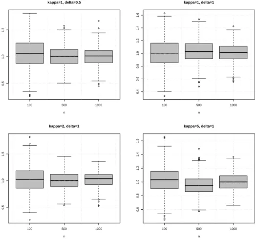
and hence the fractional order of the GH L´evy model is equal to 1. In our simulation study we simulate GH L´evy processX withβ = 0, λ= 1 and different pairs ofκ andδ atn+ 1 equidistant points {0,∆, . . . , n∆}. Upon that we construct the empirical characteristic function of increments: e φ(u) = 1 n n X k=1 eiu(Xk∆−X(k −1)∆).
Following the description of the spectral estimation algorithm, define ˜
Y(u) := log(−log(Tω−,ω+[|φe|
2](u))),
where truncation levels ω− and ω+ are constant in u and are equal to 0.01 and 0.95
respectively. In fact, for practical applications with a medium sample sizes n the choice of these levels is not crucial. Now consider the following minimization problem
(l0U, l1U) = arg min
l0,l1
Z U
0
¯
wU(u)(˜Y(u)−l1log(u)−l0)2du, (8.1)
where ¯wU(u) =U−1w¯1(U−1u) and ¯w1(u) = u1
{ǫ≤u≤1} for some ǫ >0. An estimate for the
fractional order is defined as ˜αU =lU
1. It is not difficult to show that ˜αU is of the form
˜ αU =
Z ∞
0
wU(u)˜Y(u)du
with wU(u) = U−1w1(U−1u) and w1(u) = ¯w1(u) [A
1log(u)−A2], where A1 and A2 are
two positive constants such that w1(u) satisfies conditions (6.5). LetU
1 > U2 > . . . > UK
be an exponentially decreasing sequence of cut-offs and ˜α1, . . . ,α˜K be the corresponding
sequence of estimates. Following (7.1), we construct a sequence of aggregated estimates ˆ
α1, . . . ,αˆK using a triangle kernel and a set of critical valuesV1, . . .VK computed by (7.4).
The variances {σ2
k} in (7.3) are estimated from above using a bound forζ1. Box plots of
ˆ
α = ˆαK based on 500 trials for different n and different pairs of κ and δ are shown in
Figure 8.1.
8.2
Estimation of the fractional order from options data
In the case of calibration (estimation underQ) we compute first the prices ofncall options C(yk, T) =SEQ[(eYT −eyk)+], k = 1, . . . , n
using formula (3.3), where the underlying processY follows a GH L´evy model (parameters will be specified later on), S = 1,T = 0.25 and r = 0.06. The log-moneyness design (yi)
100 500 1000 0.5 1.0 1.5 kappa=1, delta=0.5 n 100 500 1000 0.4 0.6 0.8 1.0 1.2 1.4 1.6 kappa=1, delta=1 n 100 500 1000 0.5 1.0 1.5 kappa=2, delta=1 n 100 500 1000 0.6 0.8 1.0 1.2 1.4 1.6 kappa=5, delta=1 n
Figure 8.1: Box plots of the estimate ˆα under P for different sample sizes and different parameters of the GH process.
is chosen to be normally distributed with zero mean and variance 1/3 and reflects the structure of the option market where much more contracts are settled at the money than in or out of money. Finally, we simulate
OT(yj) =OT(yj) +σ(yj)ξj, j = 1, . . . , n,
where ξj are standard normal,OT is defined in (3.2) andσ(y) = [¯σ OT(y)]2.
In the first step of our estimation procedure we find the functionOb among all functionsO with two continuous derivatives as the minimizer of the penalized residual sum of squares
RSS(O, L) = n+1 X i=0 (OT(yi)−O(yi))2+L Z yn+1 y0 [O′′(u)]2du, (8.2)
where y0 ≪ y1and yn+1 ≫ yn are two extrapolated points with artificial values On+1 =
O0 = 0. The first term in (8.2) measures closeness to the data, while the second term
penalizes curvature in the function, and L establishes a trade-off between the two. The two special cases are L = 0 when Ob interpolates the data and L = ∞ when a straight line using ordinary least squares is fitted. In our numerical example we use the R package
psplines with the choice of L that minimizes the generalized cross-validation criterion.
It can be shown that (8.2) has an explicit, finite dimensional, unique minimizer which is a natural cubic spline with knots at the values of yi, i = 1, . . . , n. Since the solution of
(8.2) is a natural cubic spline, we can write
b O(y) = n X j=1 θjβj(y)
where βj(y), j = 1, . . . , n, is a set of basis functions representing the family of natural
cubic splines. We estimate F[O](vb +i) by
F[O](vb +i) = n X j=1 θjF[e−yβj(y)](v). AlthoughF[e−yβ
j(y)] can be computed in closed form, we just use the Fast Fourier
Trans-form (FFT) and compute F[O](vb +i) on a fine dyadic grid. On the same grid one can
compute (8.3) ψ(v) :=e 1 T log 1 +v(v+i)F[O](vb +i) , v ∈R,
where log(·) is taken in such a way that ψ(v) is continuous withe ψ(e −i) = 0. Now we can
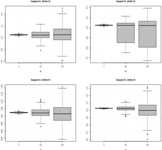
follow the road map of the adaptive spectral calibration algorithm and get an estimate for the fractional order of the underlying GH L´evy model. In Figure 8.2 box plots of the final estimate ˆα = ˆαK based on 500 Monte Carlo trials are shown in the case of the
underlying GH L´evy model with parameters β = −1, λ = 1 and different κ, δ. Sample size n is equal to 1000 and noise level ¯σ takes values in the set {1,10,20}. The estimate
ˆ
α is obviously biased because of numerical errors (due to the approximation of Fourier integral and linearization).
1 10 20 0.8 0.9 1.0 1.1 1.2 kappa=2, delta=2 σ 1 10 20 0.7 0.8 0.9 1.0 1.1 1.2 kappa=5, delta=2 σ 1 10 20 0.85 0.90 0.95 1.00 1.05 1.10 1.15 1.20 kappa=2, delta=5 σ 1 10 20 0.6 0.7 0.8 0.9 1.0 1.1 1.2 1.3 kappa=5, delta=5 σ
Figure 8.2: Box plots of the estimate ˆα under Q for different noise levels and different sets of parameters of the underlying GH L´evy process.
8.3
Processes with a non-zero diffusion part
Turn now to the class of L´evy processes containing a non-zero diffusion part which was treated in Section 6.9. The only algorithmic difference to the case of processes with zero diffusion part is that now we first fix some ξ >1 and compute
˜
Yξ(u) := log(−log(Tω
−,ω+[|ρeξ|
2](u))),
instead of ˜Y(u), where ρeξ(u) = |φ(u)˜ |2ξ
2
/|φ(ξu)˜ |2 with φebeing an estimate of φ
a. In the
estimation procedure we consider only the set of u with |φ(ξu)˜ | > 0. Note that this set is smaller than the set where |φ(u)˜ |>0 since ξ >1. It is also intuitively clear that more observations are needed to estimate ˜ρξ with the same quality as |φ(u)˜ |2 and therefore the
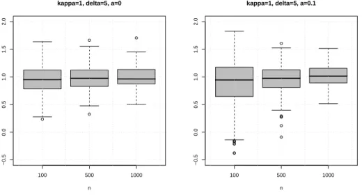
first problem is likely to be computationally more difficult. This conjecture is supported by our simulation study as well. Figure 8.3 shows the boxplots of two estimates ˆα and
ˆ
αξ based on 500 samples under historical measure P from the GH L´evy model with zero
diffusion part (left) and with the diffusion parameter a equal to 0.1 (right), remaining parameters λ, β, κ and δ being equal to 1, 0, 1 and 4 respectively. The estimate ˆαξ is
constructed from the estimates ˜αU1,ξ, . . . ,α˜UK,ξ (we use ξ = 2 and ¯w
1(u) = u1
{ǫ<u≤1} in
(8.1)) via the stagewise aggregation procedure as described in Section 7. We tookK = 30, Uk = 100(1.25)−(k−1), k= 1, . . . , K andK(x) = (1−x)1{0≤x≤1}.As to the critical values,
they are determined via (7.4) withr= 1, γ = 0.5. Note that while the difference between ˆ
αξ and ˆα is rather pronounced for small sample sizes it almost disappears for sample sizes
as large as 1000. 100 500 1000 −0.5 0.0 0.5 1.0 1.5 2.0
kappa=1, delta=5, a=0
n 100 500 1000 −0.5 0.0 0.5 1.0 1.5 2.0
kappa=1, delta=5, a=0.1
n
Figure 8.3: Box plots of the estimates ˆα(left) and ˆαξ (right) under Pfor different sample
9
Appendix
9.1
Proof of Lemma 6.1
For any positive ω− and ω+ satisfying ω−(u)≤ |φ(u)|2 ≤ω+(u), we have
Y˜(u)−Y(u)−ζ1(u)(Tω−,ω+[|
˜ φ|2](u)− |φ(u)|2)≤ ζ2(u) 2 (Tω−,ω+[| ˜ φ|2](u)− |φ(u)|2)2 ≤ ζ2(u) 2 (|φ(u)˜ | 2 − |φ(u)|2)2. Furthermore |φ(u)˜ |2−Tω−,ω+[| ˜
φ|2](u)≤|φ(u)˜ |2− |φ(u)|2, u∈Rd
and it holds on the set |φ(u)˜ |26∈[ω
−, ω+]
|φ(u)˜ |2− |φ(u)|2≥min{|φ(u)|2−ω−, ω+− |φ(u)|2}.
Thus, ζ1(u) |φ(u)˜ |2−Tω−,ω+[| ˜ φ|2](u) ≤ ζ2(u)2 |φ(u)˜ |2− |φ(u)|2 2
on the set |φ(u)˜ |2 6∈[ω
−, ω+], provided that
2|φ(u)|2|log (|φ(u)|)|min{|φ(u)|2−ω−, ω+− |φ(u)|2} ≥ |
φ(u)|4log2( |φ(u)|2) 1 +|log(|φ(u)|2)| , that is min 1− ω− |φ(u)|2, ω+ |φ(u)|2 −1 ≥ log(|φ(u)| 2) 1 +|log(|φ(u)|2)|.
9.2
Proof of Proposition 6.3
Without loss of generality we can assume thatµ= 0 in (6.8). Denote
ρ(x) = 1− sinx x ν(x),
then ρ is, up to a scaling factor, the density of some probability distribution with the characteristic functionζρψ(u),e whereζρ is a positive constant and
e
ψ(u) =
Z 1
−1
(ψ(u)−ψ(u+w))dw. Due to (6.11) the following asymptotic expansion holds
e ψ(u) =|u|ατ(u) Z 1 −1 1−1 + w u α τ(u+w) τ(u) dw =C±(α, κ)|u|α−2 1 +O(|u|−κ), u→ ±∞ with some constantsC+and C− depending onαandκ.We consider separately two cases.
Case 0< α <1 Note that in this caseψ(u) is integrable one Rand the Fourier inversion formula implies ρ(x) = ζρ 2π Z ∞ −∞
(exp(−ixu)−1)ψ(u)e du
since ρ(0) = 0. We have for any positive number a
Z ∞
−∞
(exp(−ixu)−1)ψ(u)e du= Z
|u|≤a
(exp(−ixu)−1)ψ(u)e du
+
Z |u|>a
(exp(−ixu)−1)ψ(u)e du=:I1+I2,
where |I1|.|x|.|x|1−α+κ for x→0 provided that κ≤α. Furthermore,
I2 = C±(α, κ) Z |u|>a (exp(−ixu)−1)|u|α−2du+O(|x|1−α+κ) = C±(α, κ)|x|1−α[1 +O(|x|κ)], x→ ±0 and (6.12) holds.
Case 1 ≤ α < 2 In this case we use the Fourier inversion formula for distribution functions to get Z |x|<ε ρ(x)dx= 2ζρ π Z ∞ 0 sin(εu)
u Re[ψ(u)]e du. The representation Z ∞ 0 sin(εu) u Re[ψ(u)]e du= Z a 0 sin(εu) u Re[ψ(u)]e du+ Z ∞ a sin(εu) u Re[ψ(u)]e du=:I1+I2. and the asymptotic relation
I2 = C+(α, κ) Z ∞ a sin(uε) u u α−2du+O(ε2−α+κ) = C+(α, κ)ε2−α[1 +O(εκ)], ε→+0
lead now to (6.12) provided that κ≤α−1.
9.3
Proof of Theorem 6.4
The representation ˜ αU−α = Z ∞ 0wU(u)(˜Y(u)−Y(u))du+RU,
and Lemma 6.1 imply that (9.1) E|α˜U −α|2 ≤3 E Z ∞ 0 wU(u)ζ1(u)∆(u)du 2 + 3 E Z ∞ 0
wU(u)ζ2(u)∆2(u)du
2
Let us consider the first term in (9.1) E Z ∞ 0 wU(u)ζ1(u)∆(u)du 2 = Z ∞ 0
wU(u)ζ1(u) E[∆(u)]du
2 + Var Z ∞ 0 wU(u)ζ1(u)∆(u)du . Since
ζ1(u) = 2−1|φ(u)|−2log−1(|φ(u)|) =e2η|u|
αReτ(u) /(2η|u|αReτ(u)) we have Z ∞ 0 wU(u)ζ 1(u) E[∆(u)]du = Z 1 0 w1(u)ζ 1(Uu) E[∆(Uu)]du = U−α Z 1 0 w1(u)e2ηUαuαReτ(U u)
2ηuαReτ(Uu) E[∆(Uu)]du.
(9.2)
Due to localization principle (Laplace method) and the identity E[∆(u)] = E|φ(u)˜ |2− |φ(u)|2=ε(1− |φ(u)|2),
the integral in (9.2) is asymptotically (as U → ∞) less than or equal to AεU−α
Z 1 1−δ
w1(u)u−αe2ηUαuαdu.εU−αe2ηUα with arbitrary small δ >0 and some constant A >0. Similarly
Var Z ∞ 0 wU(u)ζ1(u)∆(u)du = Z ∞ 0 Z ∞ 0
wU(u)wU(v)ζ1(u)ζ1(v) Cov(∆(u),∆(v))du dv
.εU−2αe2ηUα +ε2U−4αe4ηUα, U → ∞, where again localization principle and the identity
Cov(|φ(u)˜ |2,|φ(v˜ )|2) = 2ε3(ε−1−1)(ε−1−2)[Re(φ(u)φ(v)φ(−u−v)) + Re(φ(−u)φ(v)φ(u−v))−2|φ(u)|2|φ(v)|2]
+ε3(ε−1−1)[|φ(u+v)|2+|φ(−u+v)|2−2|φ(u)|2|φ(v)|2] are used. Turn now to the second term in (9.1)
E
Z ∞
0
wU(u)ζ2(u)∆2(u)du
2
=
Z ∞
0
wU(u)ζ2(u) E[∆2(u)]du
2
+ Var
Z ∞
0
wU(u)ζ2(u)∆2(u)du
. Since ζ2(u). | log|φ(u)|| |φ(u)|4 , u→ ∞
and
E||φ(u)˜ |2− |φ(u)|2|2 = E||φ(u)˜ |2−E|φ(u)˜ |2+ E|φ(u)˜ |2− |φ(u)|2|2 ≤ 2 E||φ(u)˜ |2−E|φ(u)˜ |2|2+ 2|E|φ(u)˜ |2− |φ(u)|2|2
. ε|φ(u)|2+ε2, u→ ∞, we get an asymptotic estimate
Z ∞
0
wU(u)ζ2(u) E[∆2(u)]du.εUαe2ηU
α
+ε2Uαe4ηUα, U → ∞. Similarly, one can prove that
Var
Z ∞
0
wU(u)ζ2(u)∆2(u)du
.ε2U2αe4ηUα, U → ∞. Finally, the third term in (9.1)
RU =
Z ∞
0
wU(u) log(Reτ(u))du can be can be bounded by
|RU|= Z 1 0
w1(u) log(Reτ(uU))du
≤ U−1 Z A 0 |
w1(y/U)||log(Reτ(y))|dy +U−κ
Z 1 0 |
y|−κ|w1(y)|dy.U−κ, U → ∞, for A >0 large enough. Combining all the previous estimates we get
E|α˜U −α|2 . εU−2αe2ηU
α
+ε2U2αe4ηUα +U−2κ
. εU−2 ¯αe2η+Uα¯ +ε2U2 ¯αe4η+Uα¯ +U−2κ, U → ∞.
(9.3)
Finally the choice
U = 1 2η+ log ε−1log−β(1/ε) 1/α¯ with β = 1 +κ/¯α leads to (6.13).
In the case of calibration problem we have |φ(u)˜ |2 = 1−2 Re " u(u+i) n X j=1 δjOe(yj)eiuyj # +u2(1 +u2) n X j,l=1 eiu(yl−yj)δ jδlOe(yj)Oe(yl) and E|φ(u)˜ |2 = 1−2 Re " u(u+i) n X j=1 δjO(ye j)eiuyj # +u2(1 +u2) n X j6=l eiu(yl−yj)δ jδlO(ye j)O(ye l) +u2(1 +u2) n X j=1 δj2σ˜2j.
As was mentioned in Section 3.2 function O(y) =e e−yO(y) is nonnegative, Lipschitz and satisfies Cram´er condition Z
R
O(y)e−ydy <∞
provided that E[e2YT]<∞. Under the condition e−A≤ kδk2 we get
Z R eiuyO(y)dye − n X j=1 eiuyjδ jO(ye j) .kδk 2 , kδk2 →0 as well as Z R eiuyO(y)dye 2 − n X j,l=1 eiu(yl−yj)δ jδlO(ye j)O(ye l) .kδk 2 , kδk2 →0. Thus, |E|φ(u)˜ |2− |φ(u)|2|.u2(1 +u2) n X j=1 δj2(1 + ˜σj2). Further |φ(u)˜ |2−E|φ(u)˜ |2 = −2 Re " u(u+i) n X j=1 δjσ˜jξjeiuyj # +2u2(1 +u2)X j<l eiu(yl−yj)δ jδlσ˜jσ˜lξjξl +u2(1 +u2) n X j=1 δ2 jσ˜2j(ξj2−1) and E(|φ(u)˜ |2−E|φ(u)˜ |2)2 . u2(1 +u2) n X j=1 δ2j˜σj2+u4(1 +u2)2 n X j=1 δj4σ˜4j.
Using these inequalities, the first term in (9.1) can be estimated from above as E Z ∞ 0 wU(u)ζ1(u)∆(u)du 2 . U8−2αe4ηUαkδk4+U4−2αe4ηUα " n X j=1 δ2jσ˜j2 #2 . ε2U8−2 ¯αe4η+Uα¯
while the second one is asymptotically negligible if ε2U8−2αe4ηUα
→0. Taking U = 1 2η+ log ε−1log−β(1/ε) 1/α¯ with β = (κ+ 4)/α¯−1, we get (6.13).
9.4
Proof of Theorem 6.5
For any two probability measures P and Q define
χ2(P, Q) =: R dP dQ −1 2 dQ if P ≪Q +∞ otherwise
The following proposition is the main tool for the proof of lower bounds in the estimation case and can be found in Butucea and Tsybakov (2004).
Proposition 9.1. Let PΘ:={Pθ :θ∈Θ} be a family of models. Assume that there exist
θ1 and θ2 in Θ with |θ1−θ2|>2δn >0 such that
Pθ1 ≪Pθ2, χ 2(P⊗n θ1 , P ⊗n θ2 )≤κ 2 <1 then lim inf n→∞ infθˆn δ −2 n max{Eθ1|θˆn−θ1| 2,E θ2|θˆn−θ2| 2 } ≥(1−κ)2(1−√κ)2,
where the infimum is taken over all estimators θˆn (measurable function of observations)
of the underlying parameter.
Taking Θ =A( ¯α, η−, η+,κ) andθi = (αi, ηi, τi), i= 1,2, we get from Proposition 9.1
sup
(α,η,τ)∈A(¯α,η
−,η+,κ)
E(|αε−α|2)≥δn−2max{E1(|αε−α1|2),E2(|αε−α2|2)}
provided that |α1−α2|>2δn>0 and
χ2(Pθ⊗1n, Pθ⊗2n)≤κ2 <1.
Turn now to the construction of models θ1 and θ2. Let us consider a symmetric stable
model
ψ(u) = iµu+ϑ(u), ϑ(u) =−η+|u|α, 0< α≤1, u∈R
For any δ satisfying 0< δ < α and M >0 define ψδ(u) = iµu+ϑδ(u),
where ϑδ(u) =−η+|u|α1{|u|≤M}− η+Mδ (1 +cM−κ)|u| α−δ(1 +c |u|−κ)1{|u|>M}.
Then φδ(u) = exp(iµu+ϑδ(u)) is a characteristic function of some L´evy process and
φδ(u) =φ(u), |u| ≤M,
where φ(u) = exp(iµu+ϑδ(u)). Indeed, the function ϑδ(u) is a continuous, non-positive,
symmetric function which is convex on R+ for large enough M and small enough c > 0. According to a well known P´olya criteria (see e.g. Ushakov (1999)), the function exp(ξϑδ(u)) is a c. f. of some absolutely continuous distribution for any ξ > 0. In
particular, for any natural n the function exp(ϑδ(u)/n) is a c. f. of some absolutely
continuous distribution. Hence, exp(ϑδ(u)) is a c.f. of some infinitely divisible distribution.
Define
and φθ1(u) = φ(u), φθ2(u) =φδ(u) with τδ,M(u) :=|u|δ1{|u|≤M}+ Mδ (1 +cM−κ)(1 +c|u| −κ)1 {|u|>M}. If Mδ = 1 +cM−κ, i.e.
(9.5) δ = log(1 +cM−κ)/logM ≍cM−κ/logM, M → ∞, then
|τδ,M(u)−1|.|u|−κ, |u| → ∞
and hence θ2 ∈Θ =A( ¯α, η−, η+,κ). Furthermore, it holds
χ2(Pθ⊗1n, Pθ⊗2n) = nχ2(pθ1, pθ2) = n Z R |pθ1(y)−pθ2(y)| 2 pθ1(y) dy,
where pθ1 and pθ2 are densities corresponding to c.f. φθ1 and φθ2 respectively. Using the
fact that the density of stable law pθ1(y) does not vanish on any compact set in R and
fulfills pθ1(y)&|y| −(α+1), |y| → ∞, we derive nχ2(pθ1, pθ2) ≤ nC1 Z |y|≤A| pθ1(y)−pθ2(y)| 2dy +nC2 Z |y|>A| y|α+1|pθ1(y)−pθ2(y)| 2dy=nC 1I1+nC2I2
for large enough A > 0 and some constants C1, C2 > 0. Using the fact that function
φθ1(u)−φθ2(u) is two times differentiable (it is zero for |u|< M) and Parseval’s identity,
we get I1 ≤ 1 2π Z R| φθ1(u)−φθ2(u)| 2du ≤ 2π1 Z |u|>M e−2η|u|α−δ du.M1−α+δe−2ηMα−δ , I2 ≤ 1 2π Z |u|>M| (φθ1(u)−φθ2(u)) ′′ |2du . Z |u|>M| u|6e−2η|u|α−δ du.M7−α+δe−2ηMα−δ .
The choice M ≍h2η1+ log ε−1log−β
(1/ε)i1/(α−δ) with ε = 1/n and some β ≥ (7−(α− δ))/2(α−δ) yields
ε−1χ2(pθ1, pθ2)<1
for small enough ε. Combining this and (9.5), we arrive at (6.14).
For the proof of lower bounds in the case of calibration one can employ the fact that the regression model
e
OT(yi) =OeT(yi) + ˜σ(yi)ξi, δi =yi−yi−1, E
is equivalent to the Gaussian white noise model
dZ(x) = O(y)e dy+ε1/2dW(y)
with the noise level asymptotics ε→0, a two-sided Brownian motion W. Here the noise level ε corresponds to the statistical regression error Pnj=1δ2
jσ˜j2. Furthermore, instead of
χ2 distance we use the Kullback-Leibler divergence
KL(Tθ1,Tθ2) = 1 2 Z R| (Oeθ1 −Oeθ2)(y)| 2ε−1dy
between two modelsTθ1 andTθ2 corresponding to two L´evy processes with characteristics θ1 and θ2 respectively (see (9.4)). Simple calculations lead to the estimate
KL(Tθ1,Tθ2).ε−1Mγe−2η+Mα−δ
with some γ >0. Hence, for small enoughε >0 it holds KL(Tθ1,Tθ2)<1
provided thatM ≍h2η1+ log ε−1log−β
(1/ε)i1/(α−δ)withβ ≥γ/2(α−δ). Assouad lemma (see e.g. Tsybakov (2008)) together with (9.5) implies (6.14).
9.5
Proof of Proposition 6.6
It holds for any fixed U
˜
αU−α =
Z ∞
0
wU(u)(˜Y(u)−Y(u))du = Z ∞ 0 wU(u)ζ1(u)∆(u)du + Z ∞ 0 wU(u)Q(u)du+RU,
where Q is defined in (6.3). As shown in Lemma 9.2 the process ε−1/2∆(u) converges
weakly to a Gaussian process Z(u) with E[Z(u)] = 0 and Cov(Z(u), Z(v)) = S(u, v). Moreover, ε−1/2Q(u)→0 almost surely. The extended continuous mapping theorem (see
Van der Vaart and Wellner (1996)) implies that if for some sequence U(ε) and finite positive real number σ
ς2(ε) =ε
Z ∞
0
wU(ε)(u)wU(ε)(v)ζ1(u)ζ1(v)S(u, v)du dv→σ2
and ς−1(ε)RU(ε) →0, then ς−1(ε)( ˜αU(ε)−α)→N(0,1).
9.6
Proof of Theorem 6.7
We give only the sketch of the proof. Let ω− and ω+ be two truncation levels satisfying
0 < ω−(u) < ρξ(u) < ω+(u) < 1 and 0 < ω− < ρξ(u)(1−log(ρξ(u))/(1 + log(ρξ(u)))).
First, similarly to the proof of Proposition 6.1 one can show that
Y˜ξ(u)−Y(u)−ζ1,ξ(u)(T0,ω+[˜ρξ](u)−ρξ(u))
≤ζ2,ξ(u)(T0,ω+[˜ρξ](u)−ρξ(u))
where
ζ1,ξ(u) = −ρ−ξ1(u) log
−1 (ρξ(u)), and ζ2(u) = 2 max θ∈{ω−(u),ω+(u)} 1 +|log(θ)| θ2log2(θ) .
Furthermore, we have on the set {ρ˜ξ(u)≤ω+(u)}
|ρξ(u)−T0,ω+[˜ρξ](u)| ≤ω+(u)
|φa(ξu)|2− |φ(ξu)˜ |2 |φa(ξu)|2 + |φa(u)|2ξ 2 − |φ(u)˜ |2ξ2 |φa(ξu)|2
and on the set {ρ˜ξ(u)> ω+(u)}it holds
|ρξ(u)−T0,ω+[˜ρξ](u)| ≤2ω+(u).
Hence E|ρξ(u)−T0,ω+[˜ρξ](u)| 2 ≤ 2|φa(ξu)|−4 E|φa(ξu)|2− |φ(ξu)˜ |2 2 + E|φa(u)|2ξ 2 − |φ(u)˜ |2ξ22
+ 4ω+2(u) P(˜ρξ(u)> ω+(u)).
Without loss of generality one can assume that there existsU0 >0 such thatρξ(u)/ω+(u)<
1/2 foru > U0.Then it holds for u > U0
P(˜ρξ(u)> ω+(u)) ≤ P
|φa(u)|2ξ
2
− |φ(u)˜ |2ξ2> ω+(u)|φ(uξ)|2/4
+ P|φa(uξ)|2− |φ(uξ)˜ |2 > ω+(u)|φ(uξ)|2/4 ≤ 16|φa(ξu)|−4 E|φa(ξu)|2− |φ(ξu)˜ |2 2 + E|φa(u)|2ξ 2 − |φ(u)˜ |2ξ2 2 .
In the case of the estimation under P, for instance, we have E|φa(ξu)|2− |φ(ξu)˜ |2 2 .ε, E|φa(u)|2ξ 2 − |φ(u)˜ |2ξ22 .ε, ε→0 and hence E|ρξ(u)−T0,ω+[˜ρξ](u)| 2 .ε |φa(ξu)|−4, ε→0.
Now one can follow the proof of Theorem 6.4 and use the fact that ζ1,ξ(u)≍c−ξ1(α)|u|−ατξ−1(u) exp(cξ(α)|u|ατξ(u)), u→ ∞.
9.7
Proof of Theorem 6.8
Instead of L´evy models θ1 and θ2 one considers models θ1,a and θ2,a with characteristic
exponents ψa(u) =iµu−¯a2u2/2 +ϑ(u) and ψa,δ(u) =iµu−¯a2u2/2 +ϑδ(u) respectively.