Multi-atlas segmentation using clustering, local non-linear manifold embeddings and target-specific templates

Local Non-Linear Manifold Embeddings and

Target-Specific Templates

CHRISTOPH ARTHOFER, BSc., MSc.

Thesis submitted to the University of Nottingham

for the degree of Doctor of Philosophy

Abstract 6

Acknowledgement 7

1 Introduction 8

1.1 Medical image segmentation . . . 8

1.2 Approaches to brain MR segmentation . . . 11

1.2.1 General overview . . . 11

1.2.1.1 Classical segmentation methods . . . 12

1.2.1.2 Higher-level segmentation methods . . . 13

1.2.2 Atlas-based segmentation . . . 14

1.2.3 Multi-atlas segmentation (MAS) . . . 18

1.3 Our approach . . . 22

1.3.1 Overview of our approach . . . 22

1.3.2 Contributions . . . 24

1.3.3 Outline . . . 25

2 Anatomical atlas building and MAS 27 2.1 Introduction . . . 27

2.1.1 Increasing the number of atlases . . . 27

2.1.2 Joint group-wise registration and segmentation methods 28 2.1.3 Patch-based methods with linear registration . . . 29

2.1.4 Reducing the computational burden . . . 29

2.2 Pre-processing . . . 30

2.2.1 Intensity inhomogeneity correction . . . 30

2.3 Image registration . . . 35

2.3.1 Similarity measure . . . 36

2.3.2 Transformation . . . 37

2.3.3 Optimisation . . . 40

2.4 Anatomical atlases and label probability maps . . . 40

2.4.1 Single-subject atlases . . . 41

2.4.2 Population atlases . . . 42

2.4.3 Unbiased probabilistic atlas construction . . . 45

2.4.4 Creation of label maps . . . 48

2.5 Tools, datasets and evaluation strategies . . . 50

2.6 Our approach to template building . . . 53

2.6.1 Pre-processing . . . 53

2.6.2 Estimating a population template . . . 53

2.6.3 Transferring the label maps to the target . . . 55

2.7 Experiments . . . 56 2.8 Discussion . . . 57 3 Target-specific template 63 3.1 Introduction . . . 63 3.2 Comparison basis . . . 67 3.2.1 Image intensities . . . 67 3.2.2 Non-image information . . . 67 3.2.3 Registration consistency . . . 68 3.2.4 Anatomical geometry . . . 69 3.2.5 Deformation fields . . . 69 3.3 Similarity metrics . . . 71

3.3.1 Basic similarity metrics . . . 73

3.3.2 Manifold learning . . . 75

3.3.2.1 Principal component analysis . . . 76

3.4 Our approach to TST building . . . 80

3.4.1 Manifold embedding . . . 81

3.4.2 TST construction . . . 83

3.5 Experiments . . . 84

3.5.1 Reconstruction of a GM image slice with eigenimages . 84 3.5.2 Reconstruction of a deformation field with eigenimages 86 3.5.3 Comparison of nonlinear dimensionality reduction meth-ods and parameter optimisation . . . 89

3.5.4 Method validation on the LONI dataset . . . 92

3.5.5 Method validation on the ADNI-HarP dataset . . . 94

3.5.6 Method validation on the IBSR dataset . . . 96

3.5.7 Method validation on the NIREP-NA0 dataset . . . 97

3.5.8 Method validation on the MICCAI 2012 dataset . . . . 98

3.5.9 Method validation on the MICCAI 2013 dataset . . . . 99

3.6 Discussion . . . 100 4 Label Fusion 103 4.1 Majority voting . . . 104 4.2 Weighted voting . . . 104 4.3 STAPLE . . . 105 4.4 SIMPLE . . . 107 4.5 STEPS . . . 107 4.6 MALP . . . 108

4.7 Joint label fusion . . . 108

4.8 Patch-based label fusion . . . 109

4.9 Our approach to propagation, fusion and binarisation . . . 111

4.10 Experiments . . . 113

4.10.1 Evaluation on the LONI dataset . . . 113

4.10.2 Evaluation on the ADNI-HarP dataset . . . 117

4.10.5 Evaluation on the MICCAI 2012 dataset . . . 126

4.10.6 Evaluation on the MICCAI 2013 dataset . . . 127

4.11 Discussion . . . 130

5 Dynamically adjusted labels 134 5.1 Offline learning . . . 134

5.2 ROI selection . . . 136

5.3 Clustering methods . . . 137

5.3.1 K-means . . . 138

5.3.2 Affinity propagation . . . 138

5.3.3 Hierarchical agglomerative clustering . . . 139

5.4 Our approach to label adjustment . . . 141

5.4.1 Dividing the labels into clusters . . . 141

5.4.2 Combining the clusters . . . 142

5.5 Experiments . . . 143

5.5.1 Evaluation on the ADNI-HarP dataset . . . 143

5.5.2 Evaluation on the MICCAI 2013 dataset . . . 146

5.5.3 Evaluation on the NIREP-NA0 dataset . . . 146

5.6 Discussion . . . 148

6 Application to Tourette’s images 152 6.1 Introduction . . . 152

6.1.1 Healthy brain development . . . 152

6.1.2 Tic disorders and Tourette’s Syndrome . . . 154

6.1.3 Method . . . 155

6.2 Results . . . 156

6.3 Discussion . . . 156

7 Conclusion and perspectives 161 7.1 Chapter overview . . . 161

Bibliography 169

Multi-atlas segmentation (MAS) has become an established technique for the automated delineation of anatomical structures. The often manually annotated labels from each of multiple pre-segmented images (atlases) are typically transferred to a target through the spatial mapping of corresponding structures of interest. The mapping can be estimated by pairwise registration between each atlas and the target or by creating an intermediate population template for spatial normalisation of atlases and targets. The former is done at runtime which is computationally expensive but provides high accuracy. In the latter approach the template can be constructed from the atlases offline requiring only one registration to the target at runtime. Although this is computationally more efficient, the composition of deformation fields can lead to decreased accuracy.

Our goal was to develop a MAS method which was both efficient and accurate. In our approach we create a target-specific template (TST) which has a high similarity to the target and serves as intermediate step to increase registration accuracy. The TST is constructed from the atlas images that are most similar to the target. These images are determined in low-dimensional manifold spaces on the basis of deformation fields in local regions of interest. We also introduce a clustering approach to divide atlas labels into meaningful sub-regions of interest and increase local specificity for TST construction and label fusion. Our approach was tested on a variety of MR brain datasets and applied to an in-house dataset.

We achieve state-of-the-art accuracy while being computationally much more efficient than competing methods. This efficiency opens the door to the use of larger sets of atlases which could lead to further improvement in segmentation accuracy.

Throughout the journey leading to this Ph.D. thesis I have been supported in various ways and influenced by many people, making it a difficult task to acknowledge each and every single one in this section.

First and foremost, I would like to thank my primary supervisor Dr. Alain Pitiot for the countless meetings and inspiring discussions, the constructive feedback and comments, and the encouragement and motivation, all of which will be missed. I would also like to send my gratitude to my second supervisor Prof. Paul Morgan for sharing his extensive scientific experience and giving valuable advice. I am very grateful for having had such kind and thought-ful supervisors. Working as an MR scanner operator alongside my Ph.D. provided complementary experience from the MR acquisition side and was made possible by Jan Alappadan Paul and Prof. Penny Gowland. Thank you also to Prof. Stephen Jackson and the James Tudor Foundation for the generous funding support and the opportunity to work in his laboratory. I hope we will cross paths again in the future. I would also like to thank my examiners Dr. Juan Eugenio Iglesias and Prof. Tony Pridmore for their time and helpful feedback.

I would like to thank my loving family, Elisabeth, Rainer, Christine, Karl and Berta for their encouragement and support despite being 1204 km away. I will be forever grateful for their continued investment and confidence in me achieving my dreams. If it was not for them this Ph.D. would not have been possible. I am also very blessed to have Filipa in my life, who has spread optimism and given me strength along the way.

Thank you to Darren, Antonis and Tom, who filled the office with a great atmosphere and to Susi, Winti, Kathi, Martina, Sebastian, Niki, Johanna and Benjamin for their unwavering friendship.

Introduction

Image segmentation is the process of partitioning an image into multiple components. While manual segmentation is time-consuming and poorly re-producible, automated methods, and in particular atlas-based segmentation, have shown to be efficient alternatives. In this chapter the aims of image segmentation and various different approaches for the segmentation of MR images will be presented. Due to our main interest in atlas-based segmen-tation methods, we will provide an overview of its basic underlying concept as well as advanced solutions followed by an outline of our approach and contributions.

1.1

Medical image segmentation

Aims of medical image segmentation: Image segmentation, in the general sense, is defined as the partition of an image into nonoverlapping homogeneous regions or objects, with respect to certain features or char-acteristics, and their separation from the background [166]. Segmentation, applied in the field of medicine and, in particular, to medical images acquired by magnetic resonance imaging (MRI), is commonly required for delineating anatomical regions of interest such as the brain, different tissue types such as grey matter or white matter, or regions associated with function, activity

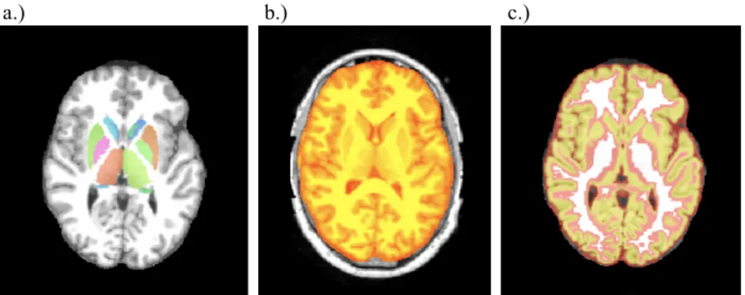
a.) b.) c.)

Figure 1.1: Aims of medical image segmentation on examples of segmented a) regions of interest, b) brain and c) grey matter.

or pathology (Fig. 1.1). It is often one of the first steps in a series of image analysis tasks such as planning of medical treatment or surgery [61, 143], diagnosis and patient follow-ups [114], and monitoring of disease progression or development [34]. Consequently, we require segmentation methods that provide accurate and reproducible results.

Challenges in image segmentation: Typically, the segmentation of an image combines two main challenges. The first is to identify certain image features like homogeneity, continuity or similarity extracted from intensity values, differences in texture or gradients in border areas (Fig. 1.2). The second challenge is to transform these extracted features into semantic en-tities and provide context. This makes it a classification task, which is one of the most difficult tasks in the image processing domain [28, 91, 210]. The segmentation of an image yields groups of voxels that belong to the same structure or region of interest, requiring each voxel of the image to be clas-sified and assigned to one of the groups. Although, over the years, various concepts have been extensively studied, the increasing number of different requirements and their associated challenges allow for no general solution which is applicable to problems from all disciplines [76].

a.) b.) c.)

Figure 1.2: Segmentation based on a.) image intensities [28], b.) gradients and c.) texture [116].

Common problems in MRI: The acquisition of images with different modalities, scan protocols or with scanners from different manufacturers, as well as the underlying physical signal acquisition itself pose challenges such as [232]:

• intensity non-uniformities, e.g. bias fields where voxels of varying in-tensities belong to the same tissue type,

• movement artefacts known as ghosting,

• partial volume effects where voxel intensities represent a mixture of different tissue types,

• frequency/phase wrapping caused by aliasing, • noise,

• poor image contrast and • weak boundaries.

All of these artefacts can have an impact of varying degree on the quality of the image processing pipeline. This makes early detection and, where possible, correction crucial.

1.2

Approaches to brain MR segmentation

1.2.1

General overview

Although manual segmentation and interpretation by experts is still consid-ered as the gold standard, it does not come without drawbacks. It is a very time-consuming and cost-intensive task, since every voxel has to be assigned a label. The segmentation accuracy is restricted by the variability introduced due to the operator(s), as different experts produce different segmentation results of the same structure (inter-observer variability). Even when the same expert performs the segmentation of an image repeatedly, variability between the resulting segmentations is introduced (intra-observer variability) [232]. An early assessment by Clarke et al. [53] outlined validation meth-ods to measure reproducibility and compared various volume measurement studies. For example, the segmentation of the hippocampus with manually supervised methods showed inter- and intra-observer variability of 14% and 10% respectively. Although technical equipment for acquisition and screen-ing of MRI and segmentation protocols such as the Harmonized Hippocampal Protocol [35, 84] have improved since Clarkeet al.’s study approximately 20 years ago, manual and manually supervised segmentation is still used as the gold-standard. An evaluation of the commonly used public dataset from the more recent MICCAI 2013-SATA challenge showed inter-scan reliability of 68% for the basal forebrain and 79% for the middle occipital gyrus, measured with the the Dice overlap coefficient [17].

In order to improve accuracy with respect to a manual gold-standard and reproducibility, a wide variety of automated segmentation algorithms have been developed. They can be classified in many ways [166] such as based on their degree of automatism (manual, semiautomatic, automatic), their spatial extent (local pixel-based, global region-based), or the concept (area-based, edge-based). Methods can also be categorised into classical (thresholding, edge-based, region-based), statistical and neural network techniques [160]. In the following sections we will give an overview of commonly used classical

and higher-level methods. In general, the former are based on low-level image processing, while the latter use classification and clustering methods which can also incorporate a priori anatomical knowledge.

1.2.1.1 Classical segmentation methods

One fast and simple method is global binary thresholding where a fixed threshold is used to split the image based on its pixels’ intensity values. Sup-port for finding the ideal threshold is given by analysing the histogram of the entire image [120, 149, 164]. This approach was further extended for multilevel thresholding [242], allowing the original image to be divided into more than two classes and local thresholding [48] for more regional decision making. In general, thresholding is simple to implement and yields fast com-putation times, but is influenced by the amount of noise, intensity contrast and anatomical complexity in the image.

In contrast, region growing aims to merge pixels into homogeneous, connected regions [2]. Every pixel in the neighbourhood around one or more starting points is examined and added to the region if a common homogeneity criterion is fulfilled. The outcome of the algorithm strongly depends on the chosen condition and is heavily influenced by the defined starting points. Conversely, instead of growing a region by merging pixels, one region can be divided into sub-regions based on a homogeneity criterion until no further splitting is possible [39]. In order to combine the advantages of both methods, a split-and-merge algorithm [103] was developed.

Another computationally efficient group of methods is based on deter-mining the edges of a structure. Commonly used edge detectors are the Sobel [192], Prewitt [158] or Canny [42] gradient operators based on first order derivatives, or the Laplacian operator based on second order deriva-tives. Due to the operators’ sensitivity to noise, smoothing the image is recommended.

The watershed algorithm [32] considers the 2D grayscale gradient or topographic distance image of the target image as a 3D surface. The grayscale

values represent heights with local minima as sources of basins and increasing values as ridges. Starting at each source, the basins are flooded. As the water rises and water sources meet, a barrier, i.e. a watershed, is created. The method tends to over-segment images, which usually requires merging of partitions in a post-processing step.

1.2.1.2 Higher-level segmentation methods

Clustering methods such asunsupervised methods aim at partitioning the data into non-overlapping groups based on certain homogeneity attributes as measured by the clustering criterion. Since each clustering technique implic-itly imposes a structure on the data, the method should be chosen carefully by considering the data under analysis. Commonly used approaches include hierarchical methods and methods based on a sum of square error criterion such as k-means [137]. Clustering methods will be discussed in Section 5.3 in more detail.

Alternatively, image segmentation can be seen as a pixel classification problem. Statistical approaches aim at characterising a structure and assigning it a category based on its features or attributes. Classifiers belong to the group of supervised methods, which discriminate new input data based on a classifier learned from a pre-labelled training set. Examples for supervised segmentation methods include active shape [63] and active appearance models[62], which are based on active contour models [54, 115] and use deforming curves or surfaces to segment a structure. These curves are controlled by internal and external forces where external forces pull the curve towards a desired object shape and internal forces preserve the local tension or smoothness of the curve.

Due to the availability of large annotated datasets neural networks (NNs) have gained a lot of attention. NNs consist of a large number of interconnected nodes, or neurons. Each neuron has a set of incoming con-nections and one outgoing connection, which represent weighted inputs and the output respectively. By organizing these networks into layers, the weights

and topological relationships between the variables can be updated and dy-namically adjust to a task, which allows the modelling of complex nonlinear relationships. Networks with multiple layers between input and output are considered as deep neural networks. One type of commonly used NNs are convolutional neural networks (CNNs) where the input image is convolved with kernels at every layer. The convolutions generate sets of features which are non-linearly transformed. CNNs usually include pooling layers where the output of previous layers is combined by applying filters. CNNs can classify each pixel individually or produce likelihood maps.

Another important and powerful high-level technique which incorporates anatomical a priori information is atlas-based segmentation [170]. In the following sections we will introduce single- and multi-atlas segmentation before presenting an overview of our approach.

1.2.2

Atlas-based segmentation

The traditional concept of atlas-based segmentation uses a single model of the human brain, which will be referred to as an atlas, to segment a new anatomical intensity brain image, referred to as the target (Fig. 1.3). The atlas, in its simplest form, consists of one individual anatomical intensity image and its corresponding label map (see Section 2.4.1). It is of impor-tance to note that in the literature the term atlas is sometimes not further specified and might refer to an individual single atlas or a probabilistic atlas. In this manuscript special care will be taken to indicate the type of atlas if not evident from the context. The target image is aligned to the anatomi-cal atlas image by estimating the spatial transformation between them using image registration. This process aims at finding the best mapping between the anatomical structures in the target and the corresponding anatomical structures in the atlas intensity image. The label maps from the atlas are transferred to the target by applying the inverse of the same transformation

Target Atlas

D-1

Figure 1.3: Single atlas-based segmentation concept.

to them. This algorithm crucially depends on the quality of the registration, which is the reason why in the literature it is often referred to as a registration problem rather than a segmentation problem. One of the first implementa-tions of this basic concept for 3-D information propagation was presented by Collinset al. [56] and Dawant et al. [69]. The advantage of their concept is its independence from the selected atlas labels, which allows the use of mul-tiple different atlas label maps without the need to re-compute the mapping between atlas- and target-space. The registration can be performed with a time-efficient affine registration or with a nonlinear method. In general a linear registration leads, without further post-processing, to a poor align-ment, and, in turn, poor segmentation quality. Commonly a combination of linear and computationally more expensive nonlinear registration methods is used, which leads to a better alignment of anatomical structures and conse-quently better segmentation results. For instance, Christensen et al. used a diffeomorphic registration method [50], which used a low-dimensional trans-formation for global shape differences and a high-dimensional vector field for the alignment of fine structures based on linear elasticity and fluidity models.

Their atlas-based model was used to automatically label a cortical surface by elastically deforming a pre-labelled 3-D surface atlas so that the cortical sulci of the atlas align with the corresponding image features in the target image [68, 179].

The segmentation accuracy crucially depends on the quality of the mapping between the target and atlas images. A one-to-one mapping between ev-ery point in the two images might not always be possible due to the high anatomical variability. Over the last decades, anatomical variability has been investigated in the whole brain as well as for particular structures showing that volume, distribution of grey and white matter, and anatomical shape vary considerably between individuals [9, 24, 152, 231]. The quality of the registration is also limited by the registration model and can lead to regis-tration errors (see Section 2.3). In an extensive evaluation, one linear and 14 nonlinear registration methods have been compared on a set of 80 man-ually labeled brain images [122]. One of the surrogate evaluation strategies measured the overlap as the agreement of deformed source and target label volumes averaged across all regions and brain pairs. A maximum overlap of approximately 71% was reached for the LONI-LPBA40 dataset [185] with the SyN registration method [21]. One way to improve registration accuracy is to use an atlas which is expected to lead to the most precise registration and, in turn, segmentation. The comparison of different atlas selection strategies has shown that an individual atlas with an intensity image more similar to the target can achieve better segmentation accuracy than the use of a randomly selected atlas [57, 85, 169]. The choice of atlas also depends significantly on the ROI [72]. While a single atlas might provide the best possible result for some ROIs it does not necessarily lead to the best outcome for other ROIs. It was concluded that there is no single atlas obtained from one individual subject that would provide the overall most accurate segmentation of a new target image. Consequently, it has been suggested to use more than one atlas to capture a wider range of inter-subject variability. In a series of studies

Atlas I1 = avg S1& L1 D . . . S2& L2 SN& LN

Figure 1.4: Probabilistic atlas-based segmentation concept.

the use of multiple individual atlases over a single individual atlas has shown improved segmentation accuracy [4, 169, 239].

One way to make use of multiple atlases is, as previously indicated, the selection of the single most similar atlas to the target from a set of atlases and its use for segmentation. Although this strategy accesses the information of multiple atlases, it eventually does not fully take advantage of all atlases. Another way to incorporate the labelling information of multiple atlases is by building an average-, population-, statistical- or probabilistic atlas (Fig. 1.4) which provides a value for each voxel indicating its probability of being part of a particular label (see Sections 2.4.2 - 2.4.3). Similar to the procedure with an individual atlas, the probabilistic atlas intensity image is registered to the target and its corresponding probabilistic label maps propagated. The use of one standardised space presents a large advantage in terms of perfor-mance. It requires only one nonlinear registration to the target at runtime and the impact of registration errors can be partly alleviated by the proba-bilistic maps. All individual atlases and registered targets are linked via their

deformation fields which makes the mapping between each of them possible by composing the respective deformation fields. In comparison, without an average atlas, computationally expensive nonlinear registrations have to be performed between each of the individual atlases and every new target.

Although computationally very efficient, the use of a probabilistic atlas has shown to provide less accurate segmentation results compared to the direct use of each individual atlas for target segmentation, which will be referred to as multi-atlas segmentation and explained in more detail in the next section.

1.2.3

Multi-atlas segmentation (MAS)

In the previous section, segmentation based on a single atlas was introduced. The single atlas of choice can either be from one individual, which, for ex-ample, could be selected as the best possible match from a set of individual atlases, or be represented as a probabilistic atlas, constructed from multiple individual atlases.

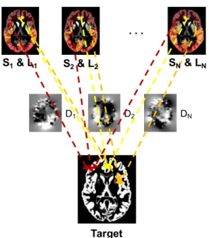
In contrast to a probabilistic atlas, Multi-Atlas Segmentation (MAS) di-rectly utilises the label information from all individual atlases of a set. A new target image is nonlinearly registered to each individual atlas resulting in as many deformation fields as there are atlases (Fig. 1.5). The same deformation fields can be applied to the corresponding atlas label maps to warp them to the target, resulting in candidate labels, which can be com-bined into the final segmentation with a label fusion algorithm. This was shown to outperform single atlas-based segmentation methods [169] and is commonly used for segmentation problems. This is in line with the findings in the pattern recognition literature where the combination of classifiers is in general more accurate than one individual classifier [38].

One of the first implementations was proposed in a series of papers by Rohlfinget al. [169, 168, 172, 173]. In their most influential work [169] they used an optimised free-form deformation algorithm to non-rigidly register

. . .

Target

D1 D2 DN

S1& L1 S2& L2 SN& LN

Figure 1.5: Multi atlas-based segmentation concept. Each individual atlas intensity image is registered to the target and each resulting deformation field is used to transform the corresponding label map to the target.

each of the atlas images to the remaining images yielding one segmentation candidate from each. The final segmentation was determined by majority voting, which assigns to each voxel the label with the most occurrences at the corresponding location in the candidate images. In [172] this simple vote rule or majority voting for the fusion of candidate labels was further extended with the expectation maximisation label fusion algorithm by Warfieldet al. [228], originally designed for the assessment of human labelling performance and estimation of the true segmentation. Since most of Rohlfing’s initial work was done on bee brains, more papers about atlas selection strategies corroborated his findings for automatic labelling of the human brain [23, 123, 239] and the impact of the label fusion method was investigated by Heckeman et al. [98]. However, most top performing MAS methods rely on the accurate alignment between each atlas and the target, which is usually done by estimating the pairwise nonlinear spatial correspondence between each atlas and the target at runtime. This step is typically the most time-consuming part of the MAS

algorithm.

Some methods have focused on running speed, e.g. Coupe et al.’s patch-based approach [64] requires only linearly aligned atlases but achieved the lowest performance in Wuet al.’s evaluation [237]. Two alternative strategies for reducing the number of registrations and improving registration accuracy either employ a target-specific template (TST), more similar to the target than an average population template [59, 61, 151, 187, 235], or construct a graph structure of intermediate similar atlas images [46, 88, 96, 110, 118, 147, 202, 225, 234] to split a large, potentially imprecise registration, into smaller more accurate deformations. However, TSTs are usually constructed as prob-abilistic atlases which does not allow the direct consultation of the warped individual atlas label maps. In most methods these probabilistic atlases are constructed from the locally or globally most similar individual atlas inten-sity images to the target by registering them iteratively to their average [59], which can increase the computational burden at runtime. Similarity mea-sures such as normalised mutual information or the sum of squared differences are commonly used for comparison of intensity images. More recent meth-ods have shown improved accuracy for candidate selection and label fusion by using distances between images calculated in manifold space [75]. Decisions solely based on image intensity values could potentially be corrputed by arte-facts or inhomogeneities. In the presence of anatomical pathology the use of deformation fields for similarity comparison is more robust [59, 61, 151, 163]. Other methods split the given labels into smaller, more localised sub-regions with the goal to improve candidate selection and fusion [18, 126, 217, 178]. However, most methods split the regions randomly without taking contex-tually meaningful information into account. One drawback of graph-based strategies is the observed decrease in segmentation overlap almost linear to the number of composed links between intermediate templates [188].

In general, eight commonly found components in MAS methods (Fig. 1.6) were identified by Iglesias and Sabuncu [105], with some of them being

op-(1) Generation of atlases (2) Offline learning (3) Registration (4) Atlas selection (5) Label propagation (6) Online learning (7) Label fusion (8) Post-processing N ove l ima ge gi ve n

Figure 1.6: Components of MAS. Optional components are indicated by the dashed boxes. Figure from Iglesias and Sabuncu [105]

tional. Given a set of atlases (1), some methods learn from or analyse the atlases offline, for example by constructing various templates or a graph structure (2). At runtime, this information is ready to use, which, in turn, improves computational efficiency. Once a target image is given, one or more atlas images are registered to it (3). Based on similarity criterions the atlas(es) with the highest expected probability of segmenting the target accurately can be selected (4) and the labels propagated (5). At runtime, another learning step can be performed (6) which can provide additional in-formation for the concurrent label fusion (7). Some algorithms additionally apply post-processing methods (8) to smooth the borders or use the fused la-bels to initialise an active contour or level set algorithm. Over the years each of these areas has become a topic of research. In this thesis, we experimented with many approaches in some of those areas, and developed our own. The next section provides an outline of our method and our main contributions.

1.3

Our approach

1.3.1

Overview of our approach

Motivated by the necessity to segment brain structures in MRI scans both accurately and in a time efficient manner, we have developed a novel MAS approach with the main aims of (1) reducing the number of nonlinear reg-istrations at runtime, and (2) providing state-of-the-art accuracy and (3) robust results on diverse datasets.

To reduce the number of registrations at runtime we use both an av-erage population template and a TST. For clarification we introduce the following notation: a ROI refers to the anatomy of interest, for example the hippocampus; a label refers to the particular delineation of a ROI, such as the hippocampus as annotated in one atlas; region refers to a collection of voxels in images or deformation fields without regards to a particular ROI; cluster refers to one sub-division of a region with similar attributes.

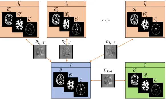
Offline, we construct a population template from a set of pre-segmented, affinely-registered atlas images and, by the same token, estimate a non-linear deformation field D between each atlas image Ieand the template G (Fig.

1.7.a). The same deformation fields are used to transform the corresponding atlas labelsLe to Gand to find clusters that undergo similar or different

de-formation. Firstly, for each location we calculate the standard deviation of the corresponding displacement magnitudes of the deformation fields. We as-sume that a high standard deviation indicates dissimilar deformation within the dataset at this location, while a low standard deviation indicates a lo-cation with similar displacement in the dataset. Secondly, we calculate the union from the labels in the space of G, which provides the largest region covered by the labels of a ROI. For each union we cluster the corresponding voxels based on their standard deviations of the deformation fields and loca-tions. The resulting set of clusters are warped back on each of the atlases, where we use the atlas labels to crop them.

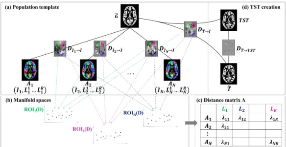
Figure 1.7: Overview of our approach. The population template G is con-structed from individual atlases offline (a). At runtime the targetTeis

regis-tered toG. A manifold embedding is constructed from the deformation fields for each ROI (b) allowing the ranking of the atlases based on their similarity to the target (c). A TST is constructed from the most similar atlas images warped onTeby composing D

e

Ij→I and DTe→I (d). Teis registered to the TST

and the atlas label maps are propagated to Te by composing D e

Ij→I, DTe→I

and D_{Te→T ST} where they are fused.

e

T to the template to obtain the target deformation field (first runtime reg-istration). For each cluster we then create a manifold embedding from the corresponding regions extracted from the atlas and target deformation fields (Figure 1.7.b). The atlas regions are then ranked in order of similarity to the target region using theirL2 _{distances in manifold space (Fig. 1.7.c). For}

each label the atlas images are then warped onto the target and a TST is constructed, to which the target is non-linearly registered (second runtime registration). We then project the label maps onto the target by composing the deformation fields between the atlases and the population template, be-tween the population template and the TST, and bebe-tween the TST and the target (Fig. 1.7.d). The resulting candidate segmentations are fused using

weights based on the rankings in manifold space which allows to determine areas with low and high probabilities. In addition to the probability val-ues, the final decision whether a voxel is part of a label is also based on the corresponding intensity value of the target by comparing it to the intensity distribution determined from high-probability areas.

1.3.2

Contributions

In order to combine the efficiency of single-atlas based methods and the ac-curacy of MAS methods we propose a novel framework with the following improvements.

First contribution: Minimising the number of registrations without compromising accuracy

(1) We reduce the number of nonlinear registrations at runtime by construct-ing an average population template from all atlas images offline (see Chapter 2) and a TST from the most similar atlas images to the target online, requir-ing only two nonlinear registrations at runtime for each new target.

(2) In contrast to other methods, the atlas images are non-linearly aligned with the target in an efficient way allowing the construction of the TST from the warped atlases on the target. This makes for an even more similar TST to the target than an average atlas or a target-specific probabilistic template constructed in average atlas space.

(3) The target is non-linearly registered to the morphologically very similar TST and by composing the deformation fields, all atlas label maps can be propagated directly to the target and consulted for fusion.

Second contribution: TST construction using region-specific man-ifold embeddings of deformation fields

(4) We create a nonlinear manifold for each ROI rather than from the whole image and from the deformation fields rather than from the intensity images

to provide the most accurate weights for the TST construction and label fusion (see Chapters 3 - 4). We evaluated two nonlinear manifold embedding strategies on a dataset with over 50 ROIs and used a more region-independent fusion method.

Third contribution: Splitting labels into meaningful clusters

5) In order to automatically select relevant sub-regions to allow for more accurate weight estimation and concurrent fusion our last contribution is the clustering of pre-defined ROIs based on the variability of the deformation. This allows the characterisation of regions that require a high and low amount of deformation at the population level (see Chapter 5).

1.3.3

Outline

In the remainder of this thesis we will discuss relevant methods from each of the components of the MAS concept (Fig. 1.6) and the impact of our ap-proach and contributions. In the beginning of each chapter we will provide a literature overview followed by a presentation of our own approach and experiments.

Chapter 2 outlines strategies for the spatial alignment of atlases with the target. We elaborate on the use of a population atlas for MAS and techniques for its creation.

Chapter 3provides an overview of computationally efficient MAS solutions. We present a fast and accurate MAS strategy that employs intermediate templates and manifold learning.

Chapter 4 introduces and compares techniques for the fusion of candidate labels and the thresholding of probabilistic segmentations.

Chapter 5 outlines strategies for offline learning to reduce the computa-tional burden at runtime and/or improve segmentation accuracy. We present our approach of using localised sub-regions which are dynamically derived

from the given atlas labels.

InChapter 6we present the segmentation results obtained by applying our method to brain MR scans of healthy subjects and Tourette’s patients.

Anatomical atlas building and

multi-atlas segmentation

2.1

Introduction

One of the essential parts of the MAS concept is the spatial alignment of the atlases with the target, which is achieved with image registration. In this chapter we provide an introduction to image registration methods, their use in MAS approaches and their effect on segmentation accuracy and runtime. In the remainder of this section we provide an overview of solutions for reg-istration in MAS and commonly used pre-processing steps, before outlining image registration methods in more detail, and techniques to create atlases and construct population templates.

2.1.1

Increasing the number of atlases

The quality of an image registration method depends on various factors such as the characteristic of the image, the ROI to be segmented and the under-lying registration algorithm and its parameters. Different methods or even the same method repeatedly applied with different parameters yield differ-ent outcomes. Similarly to the pattern recognition literature, where it has been shown that multiple classifiers yield improved and more stable results

over single classifiers [38], Rohlfing and Maurer [171] utilised these different outcomes to create a larger set of atlas-based classifiers. They repeatedly ap-plied the same registration method with different sets of parameters to the same image, with the goal of improving classification accuracy. In related work by Doshi et al. [74], multiple different image registration methods were applied to the same images, leading to a set of multiple different registra-tion results. A larger set of classifiers increased the probability of finding suitable candidates and showed superior segmentation results over using a single method. However, while a larger set of different classifiers can improve classification accuracy, the larger number of pairwise registrations with one or even multiple methods represents the most time-consuming part of MAS.

2.1.2

Joint group-wise registration and segmentation

methods

Traditionally the transformation is estimated between each individual atlas and the target, independently from the registrations of other atlases to the target. Groupwise methods [3, 97, 106, 110, 223] consider the strong reliance of the segmentation outcome on the quality of the registration and, con-versely, the potential improvement in registration quality by incorporating label information, i.e. a more precise deformation field for label propaga-tion provides better segmentapropaga-tion results and atlas labels provide impor-tant features to improve registration accuracy. For example, the generative probabilistic model by Iglesias, Sabuncu and Van Leemput [106] uses the consistency of voxel intensities within an ROI to simultaneously estimate the atlas-to-target deformation fields and target labels. In contrast to other MAS methods, these deformation fields are considered as model parameters alongside the Gaussian distribution parameters of the voxel intensities. The most likely values are estimated by a variational expectation algorithm. Al-though it can increase registration and segmentation accuracy, it can also have a negative impact on computational efficiency if all of the steps of the

method have to be re-applied for every new target image.

2.1.3

Patch-based methods with linear registration

One class of MAS methods which was originally proposed with only linearly aligned atlases is based on the non-local means method [41]. It was first utilised in MAS by Coupe et al. [64] and uses patches for the classification of target voxels (see Section 4.8). Patches around each voxel and around its neighbours in the atlas images are compared to the corresponding patch in the target image. Based on their similarity and the atlas labels at the specific location, a label can be assigned to the target voxel. Patches are selected within a specified search neighbourhood around each voxel which relaxes the one-to-one correspondences between target and atlases and makes the alignment of the images less constrained. Although proposed without the need for time-consuming nonlinear registrations, the repeated search through all of the voxels can still take a considerable amount of time and achieved less accurate results compared to other patch-based methods using nonlinear registrations. This lead to various approaches combining both nonlinear registration- and patch-based characteristics, which showed better results than the individual methods [13, 20, 25, 81, 174, 181].

2.1.4

Reducing the computational burden

The use of pairwise registrations, multiple pairwise registrations per atlas, group-wise registration, or patch-based schemes provides improved segmen-tation results at the cost of compusegmen-tational efficiency at runtime.

This computational burden at runtime can be reduced by using a common coordinate system to spatially normalise all atlases offline. At runtime, a new target requires only one registration to this same space. In the literature three main approaches for the selection of the coordinate system can be identified. Firstly, a standardised individual brain image that is not part of the atlas set can be used for normalisation, e.g. Aljabar et al. [4, 5].

Secondly, one of the atlas images can be selected as a reference space [188, 217]. However, the selection of a standardised brain image or an atlas image from the cohort might differ substantially from the remaining atlases or the target and might lead to inaccurate registration results. The third approach facilitates a population template, constructed from all atlases offline [12, 60, 61, 70, 81, 161, 187]. Although it does not guarantee similarity to the target, this approach can capture the variability within the atlas population, and, consequently, provide more accurate alignment in the average reference space.

2.2

Pre-processing

2.2.1

Intensity inhomogeneity correction

A general problem in MRI is the smooth intensity variation that can occur across the whole image. It can be caused by static field inhomogeneity and RF coil nonuniformity, and depends on pulse sequence and field strength. In most applications the correction for inhomogeneities is performed as a post-processing step by image processing tools such as SPM or Freesurfer [67] in addition to hardware-related solutions in MR acquisition. In SPM [15] inhomogeneity correction is automatically performed when segmenting an image into grey matter (GM), white matter (WM) and cerebrospinal fluid (CSF). The tissue classification in SPM is based on prior probability maps and a mixture of Gaussians model with more than one Gaussian for each class. The objective function of the model is extended by extra parameters to take intensity inhomogeneity into account. It uses a linear combination of low-frequency sinusoidal basis functions to model the spatially smooth nonuniformity. This integrated approach has shown to outperform compet-ing methods [87] and can be applied to images acquired with different pulse sequences. However, the integration of the correction method into the seg-mentation algorithm which, in turn, is based on prior knowledge about tissue types, does not allow its independent application to other anatomical

struc-tures than the brain.

A dedicated method for intensity inhomogeneity correction is nonpara-metric nonuniform intensity normalisation (N3) [190]. Although it is concep-tionally similar to SPM [130], N3 works without tissue class models, can be applied to pathological data, and is independent of the pulse sequence. The inhomogeneous field is assumed to blur the image which consequently reduces the high frequency components of the intensity distribution. The objective can be stated as finding the smooth, slowly varying, multiplicative field that maximises the high frequency content of the unblurred intensity distribu-tion. This is achieved by iteratively sharpening the intensity distribution of the blurred image and estimating the smooth field, which produces the blurred distribution, until the field converges. The smoothing operator used for N3 correction is a spline approximator. In the work by [214], this B-spline approximator was adapted to allow its use with larger field strengths, faster execution times, higher levels of frequency modulation of the bias field, and to be more robust to noise. Additionally, it utilises a multiresolution op-timisation which iteratively corrects the bias field and estimates the residual bias field.

2.2.2

Skull-stripping

One of the first steps in the neuroimage processing pipeline is often the re-moval of extrameningeal tissues, such as eyes, fat and the dura from the whole head MR images. Since the succeeding image analysis steps in the pipeline use the skull-stripped images for further processing, their accuracy is influenced by the quality of the skull-stripping method. Potential over- or under-segmentation of brain tissue can lead to errors such as imprecise esti-mations of tissue volumes or its spatial distribution. The proposed methods can be classified in two main categories, edge based and template based. Edge based techniques aim at finding an edge between brain and non-brain struc-tures. Edge based techniques are employed by the brain surface extractor

(BSE) [186] which uses an anisotropic diffusion filter, a Marr-Hildreth edge detector, morphological filter and region growing. The brain extraction tool (BET) [191] estimates a brain/non-brain intensity threshold from the image histogram and calculates a rough estimate of the centre of gravity and the ra-dius of the brain. These estimates are used to initialise a spherical tessellated surface model. Each vertex of the surface iteratively undergoes an incremen-tal movement. The movement is governed by an intensity term that finds a local threshold between brain and non-brain intensities which also takes the global thresholds into account. Freesurfer [67] uses a hybrid approach [200]. Similarly to BET, general parameters such as intensity thresholds for CSF and white matter, the centre of gravity and the brain radius are estimated. In addition, the global WM minimum location is determined, which is used as the main basin for the subsequent watershed algorithm. This results in a first estimate of the brain volume and is used to initialise a deformable surface algorithm. The active contours method iteratively deforms a tem-plate while using the brain volume from the watershed algorithm as a mask. The resulting surface is compared to a statistical atlas created from manually segmented images, which allows further refinement in case of segmentation errors. More recent algorithms also use convolutional neural networks [121], which can be trained and used on different modalities and pathologically altered head scans.

The second group of methods uses a deformable atlas with expert deleations which is registered to the target. This makes it more robust to in-tensity inhomogeneity and different acquisition protocols. A hybrid method that combines the discriminative attributes of a Random Forest classifier to detect the brain boundary and the generative attributes of a point distribu-tion model is ROBEX [104]. Offline, the Random Forest classifier is trained on a set of features derived from the voxel intensities, after intensity inhomo-geneity correction and intensity normalisation. The final classifier yields a probability volume, which indicates the probability of each voxel to be part of the brain boundary. A point distribution model is constructed from a set

of training images with corresponding landmarks. The result is a model of possible shapes which can be deformed according to the active shape model explained in Section 1.2.1.2. At runtime, a new target undergoes the same pre-processing steps such as intensity normalisation, feature calculation and voxel classification. Conceptually similar to single-atlas based segmentation, the point distribution model is fitted to the probability volume of the target with a non-linear deformation to refine the alignment. The final step involves the construction of the binary volume.

Depending on the registration approach used, MAS-based methods can be computationally more expensive and time-consuming. For example com-putational time is a limitation of Doshi et al.’s approach [73]. They used DRAMMS [150] for the nonlinear alignment of a selected study-specific tem-plate to the target because of its robustness to intensity inhomogeneities, noise, and outliers or missing anatomical regions. Eskildsenet al. presented a faster alternative [77], which is based on the nonlocal means patch-based approach and requires only linearly aligned atlases.

2.2.3

Tissue classification

In SPM spatial image normalisation (i.e. registration to a standard space template), tissue classification, and bias correction is combined in a unified model [15]. It is assumed that the distribution of voxel intensities in each set of predefined tissue classes is normal or a mixture thereof and can be described with its respective mean and variance (mixture of Gaussians). The spatial probability of GM, WM and CSF is provided by the ICBM MNI 152 atlas in a normalised stereotactic space and it is assumed that intensity inhomogeneity, i.e. a smooth varying field, is present. Due to the many unknown variables, an iterative algorithm with initial estimates, given by probability maps and a uniform bias field, was implemented. Each iteration starts by calculating the cluster parameters from the probability maps and the bias field. Then the probability maps and the bias field are updated until

convergence. In each iteration, the probability maps change slightly towards the distribution of the target image. In detail, the cluster parameters are calculated by computing the number of voxels that belong to each cluster, which further allows the calculation of the weighted mean of the image voxels and the variance for each cluster. From these cluster parameters, the prior proability images, the bias corrected field and the new label probability maps can be constructed following Bayes’ rule. The smooth varying bias field is modulated as a linear combination of low frequency discrete cosine transform basis functions.

FSL’s FAST tool [244] incorporates both a hidden Markov random field (HMRF) model and an expectation-maximisation (EM) algorithm. Over models fully specified by the histogram (finite mixture models), the MRF model has the advantage of taking spatial and, in turn, structural informa-tion into account. The spatial informainforma-tion is incorporated by a contextual constraint via a neighborhood system. The HMRF is an extension to this MRF and indicates that the states of the random field can not be directly observed. However, given a particular neighbourhood configuration and its parameters, a known conditional probability distribution can estimate them. The algorithm iterates through three EM steps, which include estimation of the class labels by MRF and maximum a posteriori (MAP), estimation of the bias field performed by MAP, and estimation of the tissue parame-ters performed by maximum-likelihood (ML). It is initialised with the mean and standard deviation for each class type, GM, WM and CSF, extracted from the histogram with Otsu’s thresholding method [149]. Since MRF and HMRF are not the main focus of this manuscript, I would refer the reader to the above mentioned literature for more details.

Like FAST, ANTs’ Atropos [22] is also based on a finite mixture model (FMM). However, a FMM assumes independence between voxels and does not take spatial and contextual considerations into account. Atropos uses prior probability models to incorporate this information and provides three options. Similar to FAST, a MRF can be used. Another way is to register

and warp labelled templates to the target to create a prior probability map. A third option in Atropos allows the user to label (sparse) points of the image, which provides an initialisation for the subsequent EM optimisation. In the E-step the label estimates for each voxel are updated based on the current estimates of the model parameters by computing the lower bound of the objective function. In the M-step the estimates of the model parameters (mean,variance) are updated by optimising this bound.

2.3

Image registration

Medical image registration has been an active area of research for over 20 years with the goal of estimating the spatial correspondence between anatom-ical structures in one image and the corresponding anatomanatom-ical structures in a second image. The result is a transformation which indicates the cor-respondence between voxels across both images. This corcor-respondence can be established by superposing landmarks or by matching voxel intensities. Landmark-based methods look for the same features in the images and try to align them with a transformation. Intensity-based methods try to in-crease a similarity measure. It is important for both approaches to define valid constraints that govern the process of finding the best images [85]. Al-though a one-to-one mapping between each of the voxels of two images would yield a perfect registration, in practice, it is very difficult to achieve because of intensity inhomogeneities, partial-volume effects, tissue motion, pathol-ogy, artefacts or simply because anatomy varies between subjects [65]. The evaluation of registration quality can be based on the use of labels [122] or features, automatically derived from the input images [193]. Both approaches are prone to errors because manually denoted labels might be inconsistent due to inter- and intra-subject variability and automatic features might not be correctly detected in complex structures with a high anatomical variability like the brain.

main components:

• Similarity or error measurement • Optimisation function

• Transformation model

In the following sections an outline of these key elements will be provided. For further details the reader may refer to [196].

2.3.1

Similarity measure

Similarity measures can be broadly categorised into three main groups: Feature-based, voxel-based and hybrid methods. Feature-based measures use geo-metric landmarks including points, lines or surfaces aiming at decreasing the (typically Euclidean) distance between corresponding features. These land-marks can be manually placed or automatically detected. Consequently, the registration accuracy largely depends on the ability of the feature extrac-tion method to find corresponding landmarks in the images. Voxel-based measures are based on image intensity values with the goal to maximise the similarity of corresponding intensity patterns. Due to this dependency, we can distinguished between intra- and inter-modal registration. Common mea-sures of similarity for images of the same modality include sum of squared differences (SSD), sum of absolute differences (SAD) and cross correlation (CC). Multi-modal image registration methods usually employ probability based methods, e.g. mutual information, which allow the comparison of im-ages in terms of information theory (entropy) with the goal to maximise the amount of information one image yields on the other [55, 138, 230]. Another approach to inter-modal registration employs a patch-based method (see Sec-tion 4.8) to measure similarity between patches in a local neighbourhood of an image and detect preserved anatomical structures [101].

2.3.2

Transformation

The transformation is the mathematical model that describes the geometric distortions that are applied to an image. Based on the chosen model and its mathematical constraints, the transformation can gain properties such as inverse consistency, symmetry, topology preservation or diffeomorphism. Inverse consistent and symmetric methods ensure that the path along which an image is transformed to a second image is unbiased by the computation direction or space of either one of the images. Consequently, the path used when registering an image A to image B is the same path when registering image B to image A unbiased by the target domain. Another desirable prop-erty for some applications is the transformation model’s ability to preserve topology. By creating a continuous and locally one-to-one mapping with a continuous inverse, folding of the grid over itself, resulting in potentially un-natural anatomical structures, can be prevented. This can also be achieved with diffeomorphisms [51, 211], which are transformation functions that are differentiable (smooth) and invertible with smooth inverses.

One linear model is the rigid-body model, which only allows rotations and translations (6 DOFs). It is a special case of the affine model, which addi-tionally allows scaling and shearing (12 DOFs). These are commonly used to correct for global shape changes, but are too constrained to describe local shape changes.

In contrast, nonrigid or nonlinear registration methods have more DOFs and can be applied to model local tissue deformations, align anatomical struc-tures that vary within a population or quantify change over time. Some of the most commonly used registration methods are based on physical mod-els and interpolation theory [196]. The former group includes elastic body models, diffusion models (Demons approaches) and flows of diffeomorphisms, while free-form deformations are an example of the latter.

Elastic body models assume that the image has similar properties to an elastic solid material, which can be modelled with the Navier-Cauchy partial differential equation [26]. The equation is governed by internal and external forces. Based on the chosen similarity measure, the external force causes the deformation, while the internal force models the stress within the elastic material. Linear elastic registration methods cannot handle large deforma-tions because the internal force of the equation increases proportionally with increasing external force making it only valid for small displacements. For large deformations, nonlinear elastic models were presented [153, 159].

Demons approaches model the transformation as a diffusion process [205]. The method considers the object boundaries in one image as semipermeable membranes, which allow the object of the second image to diffuse through them. Points on the membrane are called demons and decide whether a point of the moving object should be pushed inside or outside by iteratively computing each demon’s force and updating the transformation based on all these individual forces. One way to estimate the forces is with the optical flow equation. Thirion’s Demons approach has built the basis for a whole group of diffusion-based methods, most of which are based on the same iterative approach of estimating each demon’s forces and updating the transforma-tion based on these forces. The original model did not ensure diffeomorphic transformations which was later implemented by Vercauteren et al. [218].

Flows of diffeomorphisms estimate a displacement by integrating a ve-locity field over time with the Lagrange transport equation [51]. The veve-locity field can vary over time, which allows the esimation of large deformations as a composition of a series of small deformations [29]. Due to the integral of the velocity field along a path the deformation field is necessarily diffeo-morphic which is why this framework is also known as large deformation diffeomorphic metric mapping (LDDMM). The shortest path in the space of diffeomorphisms is called the geodesic path which allows the comparison of

distances between points or images.

DARTEL (Diffeomorphic anatomical registration using exponentiated Lie algebra) [14] is based on diffeomorphisms and allows rapid computation of the deformations due to its use of a constant velocity field and a full multigrid method which recursively goes through the scales. The use of a stationary velocity field, where the whole movement of a point over a series of time steps is integrated into a single fixed velocity field, does not allow relating each point in the flow field to the corresponding point in the brain at each time step. Starting by calculating the first and second derivatives of the objective function for a variable velocity vector field, it is thereafter constrained to constant velocity. This constraint limits the achievable diffeo-morphic configurations.

ANTs-SyN: Avants et al.’s symmetric image normalisation method (SyN) [21] extends the initially asymmetric LDDMM by guaranteeing that the geodesic mapping between two images is symmetric for every chosen similarity measure, not only for intensity differences. This is achieved by decomposing the diffeomorphism that deforms an image into a second image into two parts. Each of the images contributes equally to the whole defor-mation by constraining the sub-diffeomorphisms to be the same at half of their respective integration time, which is equivalent to half of the respective distances of the whole geodesic path. Local cross correlation was chosen as similarity measure, due to its robustness to intensity variations.

Free-form deformation (FFD) methods use a mesh of control points which can be manipulated with spline functions and consequently deform an object in the image. Different types of splines have been used where cubic B-splines [177], where adjusting the location of one control point impacts only a local neighbourhood of points, have become the most popular. FFDs have been extended by adding properties such as topology preservation and diffeomorphisms [176], symmmetry [148] and inverse consistency [79].

In a comparison by Klein et al. of 14 nonlinear registration methods [122] DARTEL and SyN were amongst the highest ranked methods in terms of overlap- and distance measures.

2.3.3

Optimisation

In most methods, the transformation is iteratively refined by estimating new transform parameter values to optimise the similarity measure of the images in the next iteration. This gradual improvement and subsequent similarity assessment is repeated until an optimum is found. The overall goal of the optimisation algorithm is to find the global optimum. One way to find an optimum is by using gradient-based techniques (gradient descent), which, however converge to a local optimum. A starting estimate close to the global optimum can be provided by reducing the capture range with a multi-scale method. By down-sampling, and then repeatedly up-sampling and register-ing the images, the transformation at each resolution level can be used as an initial estimate for the next registration step.

2.4

Anatomical atlases and label probability

maps

Due to image artefacts such as intensity inhomogeneities, partial volume effects or similarities in intensity distributions of different anatomical struc-tures, prior information is crucial for the automated segmentation of MR brain images. In atlas-based segmentation methods, this prior information is provided in form of a training dataset annotated manually by experts, which classifies it as a supervised learning method.

The first step in atlas-based segmentation requires the building of one or multiple anatomical brain atlases and their corresponding labels. It is crucial to clearly define what is considered as a brain atlas, as depending on the con-struction and application, scans from individual subjects and probabilistic

templates are often referred to as atlases in the literature.

2.4.1

Single-subject atlases

In earlier publications an atlas represented the annotation of anatomical structures and was called topological, single-subject or a deterministic atlas, with one of the most well-known examples in medicine being the Talairach atlas [201]. Talairach’s main work aimed at describing and locating anatom-ical structures not only based on their shape but also based on their location relative to each other. In his coordinate system he used the anterior commis-sure to the posterior commiscommis-sure for alignment and additionally introduced a parallel and orthogonal grid proportional to the skull size, which already provided the basis for the reconstruction of 3-dimensional volumes from 2-dimensional projections and is still widely used. With advances in imaging methodologies, more complex atlases have been developed. One represen-tative example of a deterministic whole body atlas is the Visible Human Project. CT and MRI images were obtained in addition to cryosection im-ages from whole human female and male cadavers, resulting in a complete digitial image dataset of the human body.

In a similar project, the Computerised Brain Atlas (CBA) was constructed from cryosections with the main goal to provide a brain template for nor-malisation with positron emission tomography or other imaging modes [94]. It contains 3-dimensional annotations of the brain surface, the ventricular system, the cortical gyri and sulci, as well the Brodmann cytoarchitectonic areas.

More recent atlases have been developed without the need for cryogenic images. Instead they have solely been constructed from non-invasive imaging modalities such as MR or CT scans [27, 117]. A high-resolution brain atlas was constructed by the McConell Brain Imaging Centre and used for the

BrainWeb database, which is a simulator for the creation of realistic MRI data volumes [58]. With the intention to create an average atlas with high SNR and structure definition, the Colin 27 brain atlas [102] was constructed from 27 linearly aligned scans of the same subject. However, after bringing it into stereotaxic space, it has also been frequently used as a template for alignment.

2.4.2

Population atlases

Due to the large anatomical inter-subject variability, there is no single brain anatomy scan capable of representing a whole population. Probabilistic at-lases, constructed from a set of images, have emerged as the tool of choice in the representation, analysis and interpretation of population-based imaging studies.

Population atlases provide a common 3D (stereotaxic) space for normal-isation and a reference for alignment. By mapping images from a cohort into the same space, population atlases provide a probabilistic map of the spatial location of structures of interest and an estimate of their shape (intra-population variability), allow the estimation of morphological differences be-tween distinct populations (inter-population differences) and provide support in the segmentation of new target images.

The use of probabilistic atlases has multiple advantages over individual-subject atlases:

• Since it represents the average shape and appearance of the popula-tion, it provides a space for normalisation for both the individual im-ages of the population and the targets. For the individual imim-ages, it requires the least amount of deformation to deform to their average. Consequently, for targets with similar morphological properties to the population, the quality of the registration can be increased, resulting in more precise deformation fields.

• Probabilistic atlases can be constructed for different populations, such as cohorts of different age, gender or pathology [241]. For an individual target image, the most suitable probabilistic atlas, which requires the least amount of deformation, can be selected for spatial normalisation [162, 169, 239]. On population level, the probabilistic atlases can be compared to find morphological differences.

• Three-dimensional spatial atlases can incorporate information from ad-ditional target images later on and can be extended into the time do-main, which makes it possible to compare diseases at different points in time or investigate developmental disorders [90, 156, 184].

The main goals can be defined as finding a realistic representation that cap-tures the structural and functional variability of a cohort individual scans and allowing the quantitative estimation of accuracy and errors [144].

One of the biggest attempts to create an atlas was made by the International consortium for brain mapping (ICBM) in a worldwide collaboration of imag-ing centres. Demographic, clinical, behavioural and imagimag-ing data of a total of 7000 subjects were collected, including genetic information from approx-imately 80% of the subjects. The processing steps for the construction of probabilistic brain atlases from 152 and 452 subjects included 3-dimensional intensity non-uniformity correction, and intensity normalisation. In order to create an average atlas that is spatially as well as intensity unbiased by a single subject, they were constructed from the average position, orientation, scale, and shear from all individual subjects [144, 145, 146].

The Laboratory of NeuroImaging (LONI), also part of the ICBM, constructed a probabilistic brain atlas from 40 manually delineated MRI scans of healthy volunteers. The delineation was performed for 50 cortical structures, 4 sub-cortical structures, the brainstem, and the cerebellum. These label maps were brought into a common space, which allowed the calculation of