Application of Privacy-Preserving
Clustering Methods Using Homomorphic
Encryption Algorithms
A thesis submitted to the
Graduate School of Natural and Applied Sciences
by
smail Aydn
in partial fulllment for the degree of Master of Science
in
Kindness is stronger than fear.
Application of Privacy-Preserving Clustering Methods Using
Homomorphic Encryption Algorithms
smail Aydn
Abstract
The need of protection and processing of the sensitive data in large scale data systems (for example data derived from nancial systems, militaristic systems or social media platforms) is a common problem. Usage of traditional cryptographic methods for data protection mainly needs at least two of the ciphering, deciphering and data processing works to be done on the same side. Because of this, with increase of the data size there will be a need for higher processing power to work on the data.
Using traditional encryption algorithms for protection of the sensitive data on large scale systems, also brings the need of exchanging the needed keys for protection and processing the data. Homomorphic encryption schemes have enough exibility that, they should be used on data systems that contains data from multiple parts, because of its feature of allowing to process the encrypted data like its non-encrypted form.
With the usage of homomorphic encryption schemes and proper data learning systems on encrypted data, distribution of sensitive data to dierent parties can be done without violating its privacy. In this thesis, we propose a method to run mathematical computations which needs high processing power on a common platform which oers high processing power of data but not on parties that the sensitive data will be distributed. As a result the partners of this systems will not need to have high processing power to function on the data because the high processing demanding tasks would be done on the common platform.
In this research Paillier Cryptographic system was used to protect data privacy. Paillier Cryptographic algorithm's most prominent features are its asymmetrical and partially homomorphic behavior. We proposed a system that uses privacy preserving distance matrix calculation as input for several clustering algorithms which are commonly used in machine learning systems. Our system is evaluated considering dierent data lengths and dierent key lengths. Four dierent data clustering methods have been tested. By applying clustering algorithms on both encrypted and plain forms of the same data for dierent key and data lengths, we obtained performance results by using six dierent metrics.
Homomork ifreleme Algoritmalar Kullanlarak Mahremiyet
Korumal Gruplandrma Yöntemlerinin Uygulanmas
smail Aydn
Öz
Günümüzde nans, sa§lk, askeri sistemler veya sosyal platformlarda elde edilmi³ ve mahremiyeti korunmas gereken büyük veri topluluklarnn i³lenmesi/anlamlandrlmas ihtiyac mevcuttur. Mahremiyet koruma amacyla klasik ³ifreleme yöntemlerinin kullanm, verinin kullanlaca§ sistemde ³ifreleme, ³ifre çözme veya verinin anlamlandrlmas i³lemle-rinin en az ikisinin ayn yerde yaplmasn gerektirir. Veri büyüklü§ünün artmas ile beraber bu i³lemlerin ayn yerde yaplmas durumunda büyük miktarlarda bir i³lem gücü ihtiyac do§acaktr.
Klasik anlamda kriptolama yöntemlerinin çok sayda ba§lant içeren büyük veri sistemle-rinde kullanm durumunda, i³lem yüküne ek olarak çok sayda kullancnn her bisistemle-rinde uygun anahtar da§tm mekanizmalarnn da çal³mas gerekecektir. Çok sayda kullancnn bir araya gelmi³ oldu§u bir büyük veri sisteminde gerek anahtar da§tm mekanizmalarnn ko³masnn, gerekse de büyük veri üzerinde yaplacak yüksek i³lem gücü gerektiren i³lemlerin ortak bir platform üzerinde yaplmasna imkan vermesi sebebiyle bu çal³mada homomork ³ifreleme yöntemlerinin kullanm önerilmektedir. Homomork ³ifreleme yöntemleri ile beraber ³ifreli veri üzerinde uygun makine ö§renme yöntemleri kullanlmas sayesinde büyük verilerin payda³lara da§tmnn ve veri i³lemenin mahremiyete aykr bir durum olu³turmadan yaplabilmesi mümkün hale gelmektedir.
Bu sayede sistem payda³larnn yüksek i³lem kapasitesine sahip olmasna gerek kalmadan büyük veri i³leme mekanizmalarna dahil olup, i³lem yapabilme imkanna sahip olmas sa§lanacaktr. Tasarlanan sistemin çal³masna uygun olmas sebebiyle asimetrik bir ³ifreleme algoritmas olan ve homomork özellik göstermesi sebebiyle mahremiyet koruma amacyla Paillier kriptolama sistemi kullanlm³tr. Makine ö§renme yöntemlerinin uygu-lamas amacyla tasarlanan sistem üzerinde farkl veri uzunluklar, farkl anahtar uzunluk-lar kullanuzunluk-larak mahremiyeti sa§lanan sistemde 4 ayr makine ö§renme yöntemi ko³turul-mu³tur. Her algoritmann farkl anahtar ve veri uzunlu§u için göstermi³ oldu§u performans, ayn verinin açk ve kapal halleri üzerinde ko³turulan makine ö§renme algoritmalarnn 6 farkl ölçüt üzerinden de§erlendirmeye tutulmas ile tespit edilmi³tir.
to all people who is in search of wisdom and who treats all branches
of science like their lost belongings while they keep on searching to
nd them. . .
Acknowledgments
I would like to express my sincere gratitude to my Co. advisor Dr. Ferhat Özgür Çatak for the continuous support of my study and related research, for his patience, motivation, and immense knowledge. Whenever I ran into a trouble spot or had a question about my research or writing, he consistently allowed this paper to be my own work, but steered me in the right direction whenever he thought I needed it.
I would also like to thank to Prof. Gül. I am gratefully indebted to him for his very valuable comments and guidence on this thesis.
Finally, I must express my very profound gratitude to my parents and to my spouse for providing me with unfailing support and continuous encouragement throughout my years of study and through the process of researching and writing this thesis. This accomplishment would not have been possible without them.
Thank you. . .
Contents
Declaration of Authorship ii Abstract iv Öz v Acknowledgments vii List of Figures xList of Tables xiii
1 Introduction 1 1.1 Current Situation . . . 1 1.2 Contribution . . . 3 2 Related Work 4 2.1 Related Work . . . 4 3 Preliminaries 8 3.1 Data Clustering . . . 8 3.1.1 K-Means Clustering . . . 10 3.1.2 Hierarchical Clustering . . . 11 3.1.3 Spectral Clustering . . . 12 3.1.4 Birch Clustering . . . 12 3.1.5 Evaluation Metrics . . . 13 3.1.5.1 Homogeneity . . . 13 3.1.5.2 Completeness . . . 14 3.1.5.3 V-Measure . . . 14
3.1.5.4 Adjusted Rand Index . . . 15
3.1.5.5 Adjusted Mutual Information . . . 15
3.1.5.6 Silhouette Coecient . . . 16
3.2 Homomorphic Encryption . . . 16
3.2.1 Paillier Cryptosystem . . . 17
3.2.2 Floating Point Numbers . . . 17
4 System Model 18 4.1 Development Environment . . . 18
4.2 Sequence Diagram . . . 18 viii
Contents ix
4.2.1 Client Computaion . . . 18
4.2.2 Data Authority Computation . . . 20
4.2.3 Model Building at Client . . . 21
5 Experiments and Results 24 5.1 Plaintext Results . . . 25
5.1.1 K-Means Algorithm Results . . . 25
5.1.2 Hierarchical Algorithm Results . . . 28
5.1.3 Spectral Algorithm Results . . . 31
5.1.4 Birch Algorithm Results . . . 35
5.2 Encrypted Domain Results . . . 38
5.2.1 K-Means Algorithm Results . . . 38
5.2.2 Hierarchical Algorithm Results . . . 45
5.2.3 Spectral Algorithm Results . . . 52
5.2.4 Birch Algorithm Results . . . 59
5.3 Results . . . 66
6 Conclusions and Future Work 67
List of Figures
4.1 Sequence Diagram for Client Side . . . 19
4.2 Sequence Diagram for Data Authority Side . . . 21
4.3 Sequence Diagram for Model Building at Client Side . . . 22
5.1 Plain domain clustering for dataset 500 . . . 25
5.2 Plain domain clustering for dataset 1000 . . . 25
5.3 Plain domain clustering for dataset 1500 . . . 26
5.4 Plain domain clustering for dataset 2000 . . . 26
5.5 Plain domain clustering for dataset 2500 . . . 26
5.6 Plain domain clustering for dataset 3000 . . . 27
5.7 Plain domain clustering for dataset 3500 . . . 27
5.8 Plain domain clustering for dataset 4000 . . . 27
5.9 Plain domain clustering for dataset 4500 . . . 28
5.10 Plain domain clustering for dataset 5000 . . . 28
5.11 Plain domain clustering for dataset 500 . . . 28
5.12 Plain domain clustering for dataset 1000 . . . 29
5.13 Plain domain clustering for dataset 1500 . . . 29
5.14 Plain domain clustering for dataset 2000 . . . 29
5.15 Plain domain clustering for dataset 2500 . . . 30
5.16 Plain domain clustering for dataset 3000 . . . 30
5.17 Plain domain clustering for dataset 3500 . . . 30
5.18 Plain domain clustering for dataset 4000 . . . 31
5.19 Plain domain clustering for dataset 4500 . . . 31
5.20 Plain domain clustering for dataset 5000 . . . 31
5.21 Plain domain clustering for dataset 500 . . . 32
5.22 Plain domain clustering for dataset 1000 . . . 32
5.23 Plain domain clustering for dataset 1500 . . . 32
5.24 Plain domain clustering for dataset 2000 . . . 33
5.25 Plain domain clustering for dataset 2500 . . . 33
5.26 Plain domain clustering for dataset 3000 . . . 33
5.27 Plain domain clustering for dataset 3500 . . . 34
5.28 Plain domain clustering for dataset 4000 . . . 34
5.29 Plain domain clustering for dataset 4500 . . . 34
5.30 Plain domain clustering for dataset 5000 . . . 35
5.31 Plain domain clustering for dataset 500 . . . 35
5.32 Plain domain clustering for dataset 1000 . . . 35
5.33 Plain domain clustering for dataset 1500 . . . 36
5.34 Plain domain clustering for dataset 2000 . . . 36 x
List of Figures xi
5.35 Plain domain clustering for dataset 2500 . . . 36
5.36 Plain domain clustering for dataset 3000 . . . 37
5.37 Plain domain clustering for dataset 3500 . . . 37
5.38 Plain domain clustering for dataset 4000 . . . 37
5.39 Plain domain clustering for dataset 4500 . . . 38
5.40 Plain domain clustering for dataset 5000 . . . 38
5.41 Encrypted domain clustering results for dataset 500 . . . 39
5.42 Encrypted domain clustering results for dataset 1000 . . . 39
5.43 Encrypted domain clustering results for dataset 1500 . . . 40
5.44 Encrypted domain clustering results for dataset 2000 . . . 40
5.45 Encrypted domain clustering results for dataset 2500 . . . 41
5.46 Encrypted domain clustering results for dataset 3000 . . . 41
5.47 Encrypted domain clustering results for dataset 3500 . . . 42
5.48 Encrypted domain clustering results for dataset 4000 . . . 42
5.49 Encrypted domain clustering results for dataset 4500 . . . 43
5.50 Encrypted domain clustering results for dataset 5000 . . . 43
5.51 Charts that show change of each evaluation metrics score by data length for dierent key lengths and for K-Means Algorithm . . . 44
5.52 Calculation Time Graph for KMeans Algorithm on Key-Data Length Dimensions . . . 44
5.53 Encrypted domain clustering results for dataset 500 . . . 45
5.54 Encrypted domain clustering results for dataset 1000 . . . 46
5.55 Encrypted domain clustering results for dataset 1500 . . . 46
5.56 Encrypted domain clustering results for dataset 2000 . . . 47
5.57 Encrypted domain clustering results for dataset 2500 . . . 47
5.58 Encrypted domain clustering results for dataset 3000 . . . 48
5.59 Encrypted domain clustering results for dataset 3500 . . . 48
5.60 Encrypted domain clustering results for dataset 4000 . . . 49
5.61 Encrypted domain clustering results for dataset 4500 . . . 49
5.62 Encrypted domain clustering results for dataset 5000 . . . 50
5.63 Charts that show change of each evaluation metrics score by data length for dierent key lengths and for Hierarchical Algorithm . . . 51
5.64 Calculation Time Graph for Hierarchical Algorithm on Key-Data Length Dimensions . . . 51
5.65 Enrypted domain results for dataset 500 . . . 52
5.66 Enrypted domain results for dataset 1000 . . . 53
5.67 Enrypted domain results for dataset 1500 . . . 53
5.68 Enrypted domain results for dataset 2000 . . . 54
5.69 Enrypted domain results for dataset 2500 . . . 54
5.70 Enrypted domain results for dataset 3000 . . . 55
5.71 Enrypted domain results for dataset 3500 . . . 55
5.72 Enrypted domain results for dataset 4000 . . . 56
5.73 Enrypted domain results for dataset 4500 . . . 56
5.74 Enrypted domain results for dataset 5000 . . . 57
5.75 Charts that show change of each evaluation metrics score by data length for dierent key lengths and for Spectral Algorithm . . . 58
List of Figures xii
5.76 Calculation Time Graph for Spectral Algorithm on Key-Data Length
Dimensions . . . 58
5.77 Encrypted domain clustering results for dataset 500 . . . 59
5.78 Encrypted domain clustering results for dataset 1000 . . . 60
5.79 Encrypted domain clustering results for dataset 1500 . . . 60
5.80 Encrypted domain clustering results for dataset 2000 . . . 61
5.81 Encrypted domain clustering results for dataset 2500 . . . 61
5.82 Encrypted domain clustering results for dataset 3000 . . . 62
5.83 Encrypted domain clustering results for dataset 3500 . . . 62
5.84 Encrypted domain clustering results for dataset 4000 . . . 63
5.85 Encrypted domain clustering results for dataset 4500 . . . 63
5.86 Encrypted domain clustering results for dataset 5000 . . . 64
5.87 Charts that show change of each evaluation metrics score by data length for dierent key lengths and for Birch Algorithm . . . 65 5.88 Calculation Time Graph of Birch Algorithm on Key-Data Length Dimensions 65
List of Tables
5.1 Plain domain evaluation metric scores for dataset 500 . . . 25
5.2 Plain domain evaluation metric scores for dataset 1000 . . . 25
5.3 Plain domain evaluation metric scores for dataset 1500 . . . 26
5.4 Plain domain evaluation metric scores for dataset 2000 . . . 26
5.5 Plain domain evaluation metric scores for dataset 2500 . . . 26
5.6 Plain domain evaluation metric scores for dataset 3000 . . . 27
5.7 Plain domain evaluation metric scores for dataset 3500 . . . 27
5.8 Plain domain evaluation metric scores for dataset 4000 . . . 27
5.9 Plain domain evaluation metric scores for dataset 4500 . . . 28
5.10 Plain domain evaluation metric scores for dataset 5000 . . . 28
5.11 Plain domain evaluation metric scores for dataset 500 . . . 28
5.12 Plain domain evaluation metric scores for dataset 1000 . . . 29
5.13 Plain domain evaluation metric scores for dataset 1500 . . . 29
5.14 Plain domain evaluation metric scores for dataset 2000 . . . 29
5.15 Plain domain evaluation metric scores for dataset 2500 . . . 30
5.16 Plain domain evaluation metric scores for dataset 3000 . . . 30
5.17 Plain domain evaluation metric scores for dataset 3500 . . . 30
5.18 Plain domain evaluation metric scores for dataset 4000 . . . 31
5.19 Plain domain evaluation metric scores for dataset 4500 . . . 31
5.20 Plain domain evaluation metric scores for dataset 5000 . . . 31
5.21 Plain domain evaluation metric scores for dataset 500 . . . 32
5.22 Plain domain evaluation metric scores for dataset 1000 . . . 32
5.23 Plain domain evaluation metric scores for dataset 1500 . . . 32
5.24 Plain domain evaluation metric scores for dataset 2000 . . . 33
5.25 Plain domain evaluation metric scores for dataset 2500 . . . 33
5.26 Plain domain evaluation metric scores for dataset 3000 . . . 33
5.27 Plain domain evaluation metric scores for dataset 3500 . . . 34
5.28 Plain domain evaluation metric scores for dataset 4000 . . . 34
5.29 Plain domain evaluation metric scores for dataset 4500 . . . 34
5.30 Plain domain evaluation metric scores for dataset 5000 . . . 35
5.31 Plain domain evaluation metric scores for dataset 500 . . . 35
5.32 Plain domain evaluation metric scores for dataset 1000 . . . 35
5.33 Plain domain evaluation metric scores for dataset 1500 . . . 36
5.34 Plain domain evaluation metric scores for dataset 2000 . . . 36
5.35 Plain domain evaluation metric scores for dataset 2500 . . . 36
5.36 Plain domain evaluation metric scores for dataset 3000 . . . 37
5.37 Plain domain evaluation metric scores for dataset 3500 . . . 37
List of Tables xiv
5.38 Plain domain evaluation metric scores for dataset 4000 . . . 37
5.39 Plain domain evaluation metric scores for dataset 4500 . . . 38
5.40 Plain domain evaluation metric scores for dataset 5000 . . . 38
5.41 Encrypted domain evaluation metric scores for dataset 500 . . . 39
5.42 Encrypted domain evaluation metric scores for dataset 1000 . . . 39
5.43 Encrypted domain evaluation metric scores for dataset 1500 . . . 40
5.44 Encrypted domain evaluation metric scores for dataset 2000 . . . 40
5.45 Encrypted domain evaluation metric scores for dataset 2500 . . . 41
5.46 Encrypted domain evaluation metric scores for dataset 3000 . . . 41
5.47 Encrypted domain evaluation metric scores for dataset 3500 . . . 42
5.48 Encrypted domain evaluation metric scores for dataset 4000 . . . 42
5.49 Encrypted domain evaluation metric scores for dataset 4500 . . . 43
5.50 Encrypted domain evaluation metric scores for dataset 5000 . . . 43
5.51 Encrypted domain evaluation metric scores for dataset 500 . . . 45
5.52 Encrypted domain evaluation metric scores for dataset 1000 . . . 45
5.53 Encrypted domain evaluation metric scores for dataset 1500 . . . 46
5.54 Encrypted domain evaluation metric scores for dataset 2000 . . . 47
5.55 Encrypted domain evaluation metric scores for dataset 2500 . . . 47
5.56 Encrypted domain evaluation metric scores for dataset 3000 . . . 48
5.57 Encrypted domain evaluation metric scores for dataset 3500 . . . 48
5.58 Encrypted domain evaluation metric scores for dataset 4000 . . . 49
5.59 Encrypted domain evaluation metric scores for dataset 4500 . . . 49
5.60 Encrypted domain evaluation metric scores for dataset 5000 . . . 50
5.61 Enrypted domain clustering results with dataset 500 . . . 52
5.62 Enrypted domain clustering results with dataset 1000 . . . 52
5.63 Enrypted domain clustering results with dataset 1500 . . . 53
5.64 Enrypted domain clustering results with dataset 2000 . . . 54
5.65 Enrypted domain clustering results with dataset 2500 . . . 54
5.66 Enrypted domain clustering results with dataset 3000 . . . 55
5.67 Enrypted domain clustering results with dataset 3500 . . . 55
5.68 Enrypted domain clustering results with dataset 4000 . . . 56
5.69 Enrypted domain clustering results with dataset 4500 . . . 56
5.70 Enrypted domain clustering results with dataset 5000 . . . 57
5.71 Encrypted domain evaluation metric scores for dataset 500 . . . 59
5.72 Encrypted domain evaluation metric scores for dataset 1000 . . . 59
5.73 Encrypted domain evaluation metric scores for dataset 1500 . . . 60
5.74 Encrypted domain evaluation metric scores for dataset 2000 . . . 61
5.75 Encrypted domain evaluation metric scores for dataset 2500 . . . 61
5.76 Encrypted domain evaluation metric scores for dataset 3000 . . . 62
5.77 Encrypted domain evaluation metric scores for dataset 3500 . . . 62
5.78 Encrypted domain evaluation metric scores for dataset 4000 . . . 63
5.79 Encrypted domain evaluation metric scores for dataset 4500 . . . 63
Chapter 1
Introduction
There is a need for big data[1] systems that allows users to quickly handle sensitive data which may be gathered from systems like healthcare systems or nancial systems and without violating its privacy.
Machine learning[2] is gaining a high reputation for handling valuable and private data in an ecient way on big data systems. Sometimes big data systems contain data batches related to systems that has dierent privacy policies from each other but had to be handled in a mutual way. Because of the dierent privacy policies that dierent parties have, sensitive data can't be distributed everytime.
1.1 Current Situation
It is a hard question that How can sensitive data be distributed between multiple parties without making concessions?. Classically to nd an answer to this question symmetric and asymmetric (public-private key cryptography) ciphering algorithms[3] are being used. The strength of classical cryptographic tools relies on secrecy of crypto key, strength of the algorithm and randomness that used in algorithm.
When classical ways are appealed, ciphering - deciphering works and processing the open data takes part in the same place. When it is desired to provide privacy using classical cryptographic algorithms, the parties need to have proper key or keys from public-private key pairs and the keys had to be transferred using a safe channel. As it is easy to see using this type of traditional systems, brings the need to compute all processes that need high processing power in the same place. Regrettably, this type of systems are being
Chapter 1. Introduction 2
incapable for big data systems because classical cryptographic algorithms are mainly designed for small datasets.
Data handling for machine learning algorithms while considering privacy[4] issues, primarily has two main approaches;
Firstly; using the distinctive features of big datasets for the suppression and generalization to sanitize the big data. After that, the sanitized version of data can be distributed[5, 6] or published to data parties to run any machine learning algorithm.
Secondly, using cryptographically secure multi-party computation algorithms[79] to construct protocols that can compute the same answer when obtained in private and non-private cases. This approach is applied generally when the relationship between data parties is symmetrical. Symmetrical relationship means that if the database is partitioned and distributed to parties and result of the machine learning algorithms applied to the dataset are same. So the result of the algorithm execution shows that both parties learn the same output based on the joint database.
The dierence between these two approaches is in the rst approach (sanitization approach), the parties don't execute machine learning algorithms on the data which belong to themselves and the database owner doesn't get an output of the execution. Depending on the content and the quiddity of the data there might be a need to develop a classication model that allows to work just on a specic part of the data. To develop a classication model, compute-intensive processes would be used for sanitization without violating privacy of the data. Big data classiers need an ecient for distributed learning and privacy preserving protocol. The method we will suggest aims to allow a user to create needed classiers without reaching any extra information about the data. Therefore database owner also wouldn't know anything about the data classier. Creating a data classier by means of this method would be examined through a prototype application and the performance will be observed. In this thesis, a framework will be proposed and used for applying machine learning algorithms to datasets when it is distributed and shared between parties. We will also use Paillier Cryptographic system for handling big data.
Chapter 1. Introduction 3
1.2 Contribution
In today's world the data which needs to be preserved privately can reach up to large scales and may dier in a wide range of varieties. There are several methods in literature to provide privacy for these data. Applying classical cryptographic algorithms can't be enough every time for handling privacy issues of large scale data. It is foreseen that when a process needs to run on a sensitive dataset, it is not suitable every time to send the encrypted data to dierent parties. As classical cryptographic algorithms are used for encryption, the needed processes can be executed on data only after decryption of it. This way, although data privacy is highly violated for the side where the data would be executed in, there are some mechanisms to solve this problem. Considering their competence level, it is clear that this procedure can't be used in every condition. In respect to this data privacy violation problem, there is always a necessity for a system which can both allow to preserve privacy for data and doesn't violate privacy as exposing the real data to irrelevant parties when needed process execution is performed. In this thesis, a system that uses the Paillier Cryptography for classifying big data systems and allows to handle/process the data without violating the privacy has been proposed/designed. This proposed work can be implemented to any system that gathers critical, sensitive or private information to run several processes on it. As mentioned before, health care systems, militaristic systems, nancial-commercial systems or instant private image/video processing systems. By changing used algorithms to process the data or running dierent algorithms rather than clustering algorithms, this model can be modied to make the system suitable to handle dierent needs. The proposed system would allow to use the data properly while preserving the privacy of data.
The main contributions of this research are as follows:
• Overcoming the need to use actual sensitive data for data handling is achieved by
building a model that allows to use the distance matrix of the same data instead.
• The Paillier cryptosystem encryption-based clustering model building is proposed
for preserving privacy and thus private clustering model training is achieved.
• With usage of the distance matrix of sensitive data, clustering performance of
four dierent clustering algorithms have been evaluated in respect of 6 dierent evaluation metrics and computational time.
• A system model has been oered, which allows handling high processing power
demanding tasks to be done on a powerful platform. So that the overall computational time aimed to be reduced thus it can be handled more eectively.
Chapter 2
Related Work
2.1 Related Work
In this section we will examine works related to using machine learning algorithms which depends on privacy preserving on big data systems.
Lindell Y. and Pinkas B., suggests a system which uses ID3 algorithm for data processing safety. They have stated that their system needs relatively less communication rounds and bandwidth. In this system, ID3 algorithm is used with decision tree learning and while privacy of data is preserved dierent users work on the data and then the results are merged by using cryptographic protocols [10]. The main dierence between our proposed work and this work is the used cryptographic algorithm, ID3. Lindell Y. and Pinkas B. also focused on the problem of secure multi-party computation on a joint database but, their solution for privacy is using ID3 algorithm while the projected computation on the database is decision tree learning.
Chaudhuri K. and Monteleon C., consider the balance between secrecy and learnability while designing a privacy preserving algorithm for a database. They focus on privacy preserving logistic regression algorithm. Bounding the sensitivity due to distortion is measured when a noise is applied on the system while the regularized logical regression algorithm is using a classier. A privacy-preserving regularized logistic regression algorithm is provided which is based on solving a perturbed optimization problem [11]. In their work they tried to construct a new learning method based on logistic regression to create privacy preserving linear classiers, which diers from our work that we didn't preserve privacy by our classiers, but with an homomorphic encryption algorithm.
Section 2. Related Work 5
Agrawal R. and Srikant R. state that in the future, data processing technics are going to aim on merging dierent security requirements on dierent platforms. They evaluated mathematical value of the distributed data to its original form and tried to accurately estimate the true values of the original data from distributed ones [12]. In this work the privacy is tried to be preserved by perturbing the original data by some randomization techniques, dierent from our proposed model. Also decision tree algorithms are used for classication of both original and reconstructed mutual data and these algorithms are ByClass and Local. In our work the mutual data is not perturbed for privacy and with this we also didn't need to reconstruct the original data.
Xu K. , Yue H. and their friends consider the traditional methods of cryptography for parties that doesn't share open data in respect of adequation. Due to this problem, they tried to minimize the data that needs to be processed with using the data locality feature of Apache Hadoop architecture's Map Reduce for protecting the data privacy[13], which is a big dierence from our work that we oer usage of a cryptographic protocol. While the main focus of this work is similar to our study, the approach to nd a solution for privacy preserving while handling big data is the main dierence from our work because we didn't consider a commercial platform's instruments to nd a solution but we tried to oer a general system without using any commercial platform. Also this work involves Hadoop's another feature for getting local training results, Mapper. The data locality is also a big dierence from our proposed system because this work obliges the participants of the system to handle their data locally, not on a common powerful platform. Also because this system mainly runs on the Hadoop platform, participants must use their data in HDFS (Hadoop Distributed File System) format.
Merugu S. and Ghosh J. examined the costs of security and communication of distributed data in supervised and non-supervised scenarios. The suggestion they made is to transmit the parameters of suitable generative models which built at local data sites to a central database, instead of sharing the original data. The work showed that generating articial samples from the original data distributions with using Markov Chain Monte Carlo techniques, it is mathematically possible to represent all the data with a mean model [14]. In this work, privacy is preserved by the hardness of reconstruction of the original data from the distributed model which is derived locally, no encryption algorithm is used. This work also includes distributed model clustering between dierent parties with dierent security concerns, so each party can choose a suitable expectation-maximization algorithm to use for clustering and the central "model merger" tries to nd the best solution for merging these clustering results. On the contrary of this work, in our work we oer a single data authority and the calculations are made on encrypted data because
Section 2. Related Work 6
of its homomorphic characteristic and clustering is also not done in locals.
Shokri R. and Shmatikov V. tried to use the ability of gathering information and model building of articial neural networks from complex datasets. They tried to design a practical system that allows dierent parties to jointly learn an accurate neural network model without sharing their input data. The researchers think that their system has a strong privacy compared to any existing approach due to minimal data sharing which is actually a small fraction of network parameters [15]. The usage of articial intelligence and actuating neural network algorithms are done on the client side and this is on of the dierences from our proposed model. Another dierence is, this study oers a model that uses articial intelligence which aims to work independent from the specic algorithm which is used on training data. Also dierent from proposed system, participants of this system share their models with each other,so participants may also learn from other participants' models.
Yang et al. oer a system that allows users to use a model for calculating data frequencies which also preserves privacy. The main logic of the system is to calculate the frequencies of specic values or a group of values of client side's data at the data mining side and while doing it data privacy is still protected by ElGamal cryptographic algorithm. It has been stated that there is no information shared except frequency of data values [16]. This work is focusing mainly on the scenario that participants of the system doesn't want to use the result of the data mining procedure which is the most prominent dierence from our proposed system that inn our system client wants to use the clustering result. Another dierence is thgis work also aims on calculating the frequencies of specic values of the data of client side but, our model clusters data using certain clustering algorithms.
Sahin O.D. , Agrawal A. and El Abbadi A. oer a system that guarantees the data of a party which doesn't pertain to another data source won't be revealed. To provide the privacy and build a distributed decision tree learning algorithm, ID3 algorithm and Shamir's secret sharing are used [17]. Their work diers from our model by the algorithm used for privacy which is Shamir's secret sharing and the algorithm runs on the data aiming to create decision trees which is ID3 algorithm. Dierent from our work, this work is proposing a non-homomorphic algorithm for data privacy and constrains the client to use it three times successively on dierent calculation phases, but we propose a system model that uses homomorphic algorithm and the clustering algorithms run on the encrypted data so encryption and decryption costs are signicantly lower.
Section 2. Related Work 7
Li et al. suggest usage of multi key-fully homomorphic encryption as well as a hybrid structure which combines double decryption with fully homomorphic encryption. They tried to prove that these two privacy-preserving algorithms are proper to use with deep learning algorithms over encrypted data. Dierent users choose their keys and encrypt their data. Encrypted data is sent on a cloud and the execution on the data is made by these two suggested systems [18]. Dierent from our model, this work mainly focuses on the issue of collaborative deep learning. Also we use a classical encryption-decryption routine in our model but in this work, to preserve privacy double decryption is oered not only to protect the data, but also to protect the model that every participant of the system created from their data.
Yi X. and Zhang Y. considered a privacy preserving Bayes classier method for horizontal-ly partitioned data and proposed two protocols. One of these protocols are two-party protocol and the other one is a multi-party protocol. Multi-party protocol is used between owners of sensitive data and a semi trusted server while two party protocol just broadcasts the classication result. In this work it is assumed that these two protocols are trusted and can preserve privacy [19]. This study diers from our proposed model by the used classication protocol which is naive Bayes classication. While we propose a model that preserves privacy by using a homomorphic encryption algorithm, Paillier cryptographic system, this study aims for the same objective by enhancing the Bayes classication model oered by Kantarcioglu and Vaidya.
Secretan J. , Georgiopoulos M. , Koufakou A. and Cardona K. approached the hardness issue of developing a privacy preserving data mining (PPDM) algorithm. PPDM algorithm are computationally intensive to execute and there is a need in the data mining that developers need convenient abstraction algorithms for simplication of the system. Dier-ent from our work, this study focuses on using parallel computing between dierDier-ent organizations and it is advised in their study because of its ability to bring high performance and that can bear on the computationally intensive works of data mining. Their study mainly considers a system built on the idea of in one tier a simplied use of cluster and grid resources would exist and at another tier the system would just abstract the communication for algorithm development [20]. This study mainly diers from our work by two reasons. Firstly, its main focus is trying to integrate a high performance and parallel computing environment between dierent organizations and secondly it suggests usage of APHID (Architecture for Private and High-performance Integrated Data mining) because of the lack of middleware frameworks that organizations would need to support PPDM.
Chapter 3
Preliminaries
In this chapter, we will briey examine on data clustering, clustering methods, homomor-phic encryption and Paillier Cryptosystem.
3.1 Data Clustering
Clustering can be described as dividing accumulated elements[21] into dierent groups depending on special features they have. Elements that are similar with each other should be in the same group as much as possible. Same logic is a subject on clustering algorithms aiming to work together with data mining algorithms.
Clustering analysis has been originally used in anthropology by Driver and Kroeber[22, 23] and then introduced to psychology by Zubin. So, clustering may be done using dierent methods due to dierent needs and dierent logical reasons with compliance to several exibilities. Some of these methods can be described as,
Centroid-Based Clustering: Centralized clustering or centroid-based clustering[24, 25] represents a group by a central vector which doesn't have to be a member of the dataset it belongs. This method comes up with a problem: How many clusters there should be? This question is the main drawback of data mining algorithms that depends on this method (such as K-Means algorithm) and common approach to this problem is to nd approximate solutions. After deciding cluster numbers, then central vectors for each cluster is calculated by squared distances from the clusters to nd nearest elements to form clusters. Due to this logic the squared distances from center should have their
Section 3. Preliminaries 9
minimal value.
Distribution-Based Clustering: In this method elements of a big dataset is clustered due to the statistical model they create[26]. Clusters can be dened as elements belonging most likely to the same distribution. This method can be considered as an excellent method theoretically but it suers a main problem known as over tting. One prominent mixture model that is in use with this method is Gaussian mixture[27]. Dataset
is initially modeled with a Gaussian distribution randomly then the parameters are
optimized to t the dataset better. This will converge into an optimum model, so iteration is needed to nd the best model. Distribution-based clustering models are good for capturing correlation and dependencies between samples although it brings an extra burden on the user in terms of iterative computing.
Density-based clustering: When clusters are dened considering the areas of high density of elements in a big dataset, that method is density based clustering[28, 29]. Methods that use density-based clustering use dierent criterion for dening the density. One of the most popular criterion is called as 00density reachability00 [30]. This logic works in
the way of searching for elements in a dataset which are within a certain threshold value and adding those elements into a same cluster. There are dierent algorithms that can forms clusters according to same-density data and because of the working logic these algorithms have they can form arbitrarily shaped clusters on the contrary of many other clustering algorithms.
Connectivity-based clustering: This clustering method relies on the idea of clustering logic which collects elements of a big dataset that are more related to nearby elements than elements farther away and form a cluster[3133]. This method forms clusters according to their distance, so a cluster can be described by the maximum distance needed to collect elements. Dierent clusters will form at dierent distances, so this model can be represented with a00dendrogram00[34] because these algorithms provide a hierarchical
model that within a certain model clusters also merge with each other. Distance values that are in use for clustering can be calculated or selected due to dierent needs. For example distance that will be used for clustering can be minimum or maximum distances between elements or average distances between them.
Dierent clustering algorithms can be used according to the chosen clustering logic. In our work, we analyzed four dierent clustering algorithms in respect to dierent logical approaches which are described above and working procedure of these algorithms will be
Section 3. Preliminaries 10
explained below together with the method they use while clustering a dataset.
3.1.1 K-Means Clustering
K-Means clustering method[35] creates clusters from a dataset according to previously determined cluster number (n clusters) and while doing that, clustering is done in according to have nearest 00inertia00 values for every cluster. Inertia value is calculated
as sum of squared distances between the central point of a cluster and every other point inside the same cluster. This algorithm is generally useful for big datasets and is used in many dierent applications[36]. K-Means algorithm divides a set of N samples into K disjoint clusters while cluster centroids are and the other points inside a cluster are X. K-Means algorithm aims to choose centroids that minimize the inertia in accordance with the equation of:
n
X
i=0
min(||x−µi||2) (3.1)
Inertia, or the within-cluster sum of squares, can be used to measure how internally coherent clusters are. This criterion also suers from several conditions. For example it is usually assumed that the dataset is 00complex00 and 00isotropic00 but unfortunately
it isn't always the case, so it makes inertia inecient to elongated clusters or irregular shaped datasets. Furthermore, while smaller values are better and the best case is when the value is 0, on high-dimensional datasets Euclidean distances[37] tend to become inated. This situation is named as00curse of dimensionality00. To speed up K-Means
algorithm and alleviate this problem, dimensionality reduction algorithms can be used before running K-Means algorithm on a dataset.
To get the best clustering results, K-Means algorithm should run on the same dataset multiple times[38]. Because of the need for high processing power and speed, we suggest that computations such as these algorithms should run on a powerful cloud environment to eliminate the case that users shall provide that much of processing power to the system. After enough time, K-Means algorithm will always converge to a local minimum value.
K-Means algorithm will initially create clusters by grouping elements around chosen central points and according to inertia values of these clusters. As the iteration goes on, algorithm shifts central points and re-group elements into clusters and calculate new inertia to converge into a minimum value. As it easy to see, it is important to choose accurate central points at the initialization of computing because more accurate cluster centroids will signicantly reduce time or number of iteration to get better clustering.
Section 3. Preliminaries 11
3.1.2 Hierarchical Clustering
Hierarchical clustering is a general name for certain clustering methods that builds nested clusters by merging or splitting their elements. These clustering methods create clusters with a logic similar to root-tree structure. The hierarchy of clusters can be represented as a tree shape (dendrogram) while the roots of the tree represent clusters and leaves
represent only one sample that collect some clusters under itself.
Hierarchical algorithms can be expressed under two main titles, Agglomerative clustering and Divisive clustering algorithms. In our work we used Agglomerative Clustering method and this method works with a bottom-up approach like root to tree logic, unlike Divisive clustering method. The way that Agglomerative clustering method will follow for clustering depends on the clustering number which is predetermined and the method the algorithm will use[39]. These methods are:
• Ward: For every group, calculation of inertia is an issue like in the K-Means
Clustering but usage of this value is dierent from K-Means algorithm due to structure of Agglomerative clustering. It aims to minimize the inertia dierences within all clusters.
dij =d({Xi},{Xj}) =||Xi−Xj||2 (3.2)
• Maximum or Complete Linkage: Clustering is done with consideration of minimizing
the maximum distances between dierent clusters. While the distance between clusters isd, the logic of this method can be described as:
max{d(x, y) :x∈A , y ∈B} (3.3) • Average Linkage: Minimizing the mean distance between pairs of clusters are used
for clustering. For example, while x and y represent points belonging to dierent clusters, the equation to calculate the mean distance between cluster A and cluster B is as: 1 |A|.|B| X x∈A X y∈B d(x, y) (3.4)
Section 3. Preliminaries 12
3.1.3 Spectral Clustering
Spectral clustering mainly work on to embed the anity matrix between samples[40], followed by a clustering algorithm. This method is especially ecient on relatively small datasets or if the anity matrix is sparse and the dataset is convex[41]. This algorithm needs cluster number to be specied before working on the dataset.
3.1.4 Birch Clustering
Birch algorithm[42] builds a tree called the characteristic feature tree (CFT). CFT structure consist of characteristic feature nodes (CFN) and these CFNs are made of characteristic feature sub-clusters (CFS). With the information gathered from characte-ristic feature sub-clusters, which is the subsidiary of CFT tree, there is no need to save the entire data on the memory to create clusters from the dataset. Birch algorithm also brings eectiveness to memory use on the platform it runs and it is done by holding some information about the dataset. Some of these informations are:
• Number of samples in a sub-cluster.
• Linear Sum: A n-dimensional vector holding the sum of all samples • Centroids: This avoids recalculation of linear sum for n samples • Squared Sum: Squared norm of the centroids.
Birch algorithm primarily needs two information to cluster the dataset. These are threshold value which will be the radiant of clusters which puts a limit for clusters and branching factor which denes maximum number of elements that every cluster can have. Birch algorithm can only work on dataset after gathering these information. After the clustering is done, if a new sample is inserted into the dataset, it is then merged with most proper sub-cluster constrained by the threshold and branching factor conditions. If the radius of the sub-cluster obtained after the merging the new sample and the branching factor is exceeded, then a new space shall be allocated for this new sample. In this condition the easiest solution to this can be splitting the most suitable cluster into two (if it doesn't result in exceeding the cluster number) [43].
Section 3. Preliminaries 13
3.1.5 Evaluation Metrics 3.1.5.1 Homogeneity
Homogeneity criteria can only be satised if members of each single class are placed into a distinct cluster in terms of homogeneity[44]. So that each cluster signicantly contains only members of a single class. The class distribution within each cluster should be done from a single class. Homogeneity gets a value between 0 and 1. For a perfect clustering, the homogeneity value gets the value 1.
AsY represents the data which belongs to the same class andT represents the clusters
that the data would be clustered into, homogeneity value can be expressed as H(Y|T).
The value ofH(Y|T)is dependent on the size of the dataset. We use homogeneity value
by its normalized form by H(Y) instead of its raw entropy value. While H(Y) could
provide the maximum homogeneity value, this form can be expressed as;
(H(Y|T))
(H(Y)) (3.5)
In a perfect homogeneous situation, this normalization,(H(Y|T))
(H(Y)) equals to 0. Thus, as we
know that 1 is desirable and 0 is undesirable condition, the homogeneity can be dened as: h= 1 ifH(Y, T) = 0 1−HH(Y(Y|T)) else (3.6)
Where a dataset that consists of N data points and these data points belongs to Y
number of classes which varies betweenc= 1, ..., Y and placed intoT number of clusters
which varies between k= 1, ..., T. xck shows the number of data points belongs to the
classc and is also an element of clusterk. nshows the quantity of number of classes.
H(Y|T) =− |T| X k=1 |Y| X c=1 xck N log xck P|Y| c=1xck H(Y) =− |Y| X c=1 P|T| k=1xck n log P|T| k=1xck n (3.7)
Section 3. Preliminaries 14
3.1.5.2 Completeness
This metric, which is symmetrical to the homogeneity metric, expresses the proportion of data belonging to the same class within the same dataset[44]. If the data belonging to the same data class is included in the same group as the result of the clustering of the dataset, this metric which takes the ideal value in this situation regarded as 1, if the grouping is farthest from ideal, the value of this metric will be 0.
In order to satisfy this criterion each of the clusters should comprise of elements which belongs only one class. Distribution of cluster assignments within each class is used to evaluate completeness. As Y represents the data which belongs to the same class and T represents the clusters that the data would be clustered into, completeness value can
be expressed as H(T|Y). In ideal condition H(T|Y) = 0. The worst case scenario is
when each class is represented by each cluster and in this case H(T|Y) = H(T) = 1.
Completeness can be dened as:
c= 1 ifH(T, Y) = 0 1−HH(T(T|Y)) else (3.8)
Where a dataset that consists of N data points and these data points belongs to Y
number of classes which varies betweenc= 1, ..., Y and placed intoT number of clusters
which varies between k = 1, ..., T, ack shows the number of data points which is an
element of cluster k and is also belongs to the class c. nshows the quantity of number
of classes. H(T|Y) =− |Y| X c=1 |T| X k=1 ack N log ack P|T| k=1ack H(T) =− |T| X k=1 P|Y| c=1ack n log P|Y| c=1ack n (3.9) 3.1.5.3 V-Measure
V-Measure is a criterion which measures how successfully did homogeneity and complete-ness criteria have been satised[44].V-Measure is calculated by taking the harmonic mean of the homogeneity and completeness metrics. This criterion takes values between 1 and 0. As described above in homogeneity and completeness sections, these two metric have working logic that are opposite to each other. Increase in homogeneity results in decrease in completeness, and vice versa. V-Measure can be calculated as:
Section 3. Preliminaries 15
v−M easure= (2×homogenity×completeness)
(homogenity+completeness) (3.10)
3.1.5.4 Adjusted Rand Index
A metric called 00Rand Index00 which is a measure of similarities between two data
clusterings, should be calculated in order to get 00Adjusted RandIndex (ARI)00[45].
While Rand Index may vary between 0 and 1, Adjusted Rand Index can also yield negative values. Rand index which is calculated separately for both the clustering which is expected to be ideal and the clustering that is currently made, and then these index values are used in the formula below to00adjust00 the Rand Index:
ARI = (RI−E(RI))
(max(RI)−E(RI)) (3.11)
E(RI) shows the expected value which is a result of a set of calculations obtained from a contingency table which is formed by amount of the objects of the dataset which had been put in the same or dierent clusters with the compared clusters.
Adjusted Rand Index gets its perfect score when the clustering is random and independent of number of clusters, than the score would be 0. On the contrary if the clusters are identical and/or similar to each other, then the index becomes 1. This metric is symmetrical. So:
ARI(x, y) ==ARI(y, x) (3.12)
3.1.5.5 Adjusted Mutual Information
This metric is also an adjusted metric like ARI. Mutual information tells us how much information is shared between dierent clusters and this metric measures this information. So, adjustedmutualinf ormation [46] can be considered as a similarity
measure. In our work this metric measures the number of mutual elements between dierent clusters. This metric is equal to 1 when the clusters are completely identical, and when clusters are independent from each other this metric becomes equal to 0. That means there is no information shared. Adjusted Mutual Information is the adjusted form of mutual information. The mutual information value is adjusted as below where U and K are the clusterings which will be under the scope:
AM I(U, T) = I(U, K)−E(M I(U, K))
Section 3. Preliminaries 16
E(M I(U, K))shows the expected value which is a result of a set of calculations obtained
from a contingency table which is formed by amount of the objects of the dataset which had been put in the same or dierent clusters with the compared clusters.
This metric is also symmetrical like adjusted random information.
3.1.5.6 Silhouette Coecient
Silhouette coecient[47] is calculated by using both intra-cluster distance and mean nearest-cluster distance which is the distance between a sample and the nearest cluster that the element is not a part of for each of the elements in a dataset. The formula is:
Silhouette Coef f.= (y−x)
max(x, y) (3.14)
where y is the distance between an input instance and the nearest cluster which the
instance doesn't belong and x is the mean value of distances within the cluster which
the instance is a part of. To calculate the Silhouette coecient, the dataset should have at least two clusters. This metric returns the mean value over all calculated Silhouette coecient values for instances in dataset.
Silhouette coecient varies between -1 and 1. When this metric is considered for an instance the more Silhouette coecient is closer to -1, the more likely the instance is in wrong cluster. If this metric is considered for all dataset the more the value gets closer to -1, the more clustering isn't accurate and instances are more likely misplaced and clustering had put instances in clusters which they should not belong. On the contrary, the more this metric gets closer to 1, the more likely the clustering is accurate. When the value of this metric near 0, then probably clusters are overlapped.
3.2 Homomorphic Encryption
Homomorphic encryption is a form of encryption method that allows computation on encrypted data and generates result which would have been same result if the same computation would be performed on the plain data. As it can be seen from this main property of the method, the purpose of the method is to preserve privacy[48 51] . Homomorphic encryption can also be used in connecting dierent services without exposing their sensitive data. Homomorphical encryption algorithms can be expressed in two groups as partially homomorphic algorithms and fully homomorphic algorithms[52]. In our work, we used Paillier Cryptosystem and this is a additive partially homomorphic algorithm[53].
Section 3. Preliminaries 17
3.2.1 Paillier Cryptosystem
Paillier cryptosystem[54] is an asymmetric , probabilistic and public key cryptosystem. It preserves privacy[55] depending on diculty of the problem of computing the n-th residue classes. Paillier cryptosystem is a additive partially homomorphic system, that means encryption ofM1 andM2 plain datasets with aKpublic key gives the same result
as the encryption of addition of same two dataset (M1 +M2) with using the same K
public key. This encryption algorithm works by doing two main jobs in an order, rst one is key generation and the second one is encryption/decryption of dataset.
As explained before Paillier Cryptographic system has homomorphic properties which makes this algorithm more convenient to be used in several elds. These properties are:
• Addition of encrypted data: Result of adding of two encrypted datasets matches
with the result of enciphering and adding two datasets.
• Multiplication of encrypted data with a non-encrypted value: Multiplying an
encrypted data with a number N is same with multiplying the plain form of that
data with the same numberN and encrypting it.
3.2.2 Floating Point Numbers
In this work, oating point numbers are used to express data which has been encrypted using Paillier Cryptosystem in the python environment and to express the values in the datasets we used in this work. As a natural consequence, the operations on the data are also based on the values dened in this type.
The number of digits in the fraction part of the data that is dened as oating point can be very large and if these numbers would be used than it would denitely cost more processing power and processing time, so in this work only the rst 5 fractional digits have been used. Because of the 5 digit limit has been put on the fractional digits of input data and more than these digits are not used, which has been possibly generated as a result of computational work, are rounded into 5 digits and this situation possibly creates minimal data losses or deviation of computation [56]. It is seen that these eects on the calculation result depends on the grouping algorithm used, but overall it is low in eectiveness [57].
Chapter 4
System Model
4.1 Development Environment
In this thesis, Python 2017.3.3 community edition is used for algorithm programming which encrypts data using Paillier cryptography and makes clustering using 4 dierent algorithms which have been described in section 3. Each algorithm run on a computer which has Intel(R) Core(TM) i7-6700HQ CPU @ 2.60GHz octa core processor (4 real +4 pseudo) along with 16GB of RAM. Parallel computing has not been used everytime but while some algorithms allow to use all processor cores while running, that property has been used.
4.2 Sequence Diagram
In this section, the system which is designed to preserve privacy while handling private or sensitive data is explained by sequence diagrams. This system doesn't only aim to preserve privacy, but also aims to handle the data eciently in terms of time and processing power.
4.2.1 Client Computaion
Client side doesn't hold the data which needs to be handled, because management and maintenance of a big data storage brings unnecessary extra cost. In this work client of this system is considered as an ordinary PC user, so there is no data storage for big data systems on client side and the main task of client side is just using/handling sensitive data when it is needed. The client generates public and private key pair by establishing a
Section 4. System Model 19
key exchange session with data authority, then sends its public key and asks for the data needed. As the data needs to stay encrypted and not revealed to client,at this point, data computing cloud starts to handle the data.
Data Computing cloud also doesn't store the sensitive data but preserves enough processing power for handling the encrypted data. On computing cloud servers, the mathematical computations run to compute an encrypted distance matrix from the encrypted data in a form that can be used by the client. Cloud servers perform needed calculations for client side without violating the data privacy and sends the results, which is in our case the encrypted distance matrix. Client side then uses the encrypted matrix in order to build a model and evaluate the data. As seen in Figure 4.1, in this system client side doesn't need the actual data to use because enough information can be derived from the distance matrix. Data Authority Data Producing App. Data Computing Cloud Calculation App. Data Using Environment Client M1: Generate Keys Crypto Key(pub),
Key(priv)
M2: Key Exchange CryptoKeypub
M3: Call for Encrypted Data(Xenc m )
M4: Send Encrypted Data (Xenc m )
M5: Calculate Enc. Distance Matrix Hmenc
M6: Send Distance Matrix (Hmenc)
Figure 4.1: Sequence Diagram for Client Side
The pseudo code for Client Computation part of the system is shown in Algorithm
1. In key generation step, pseudo code doesn't contain explanation of step-by-step key generation. As the Paillier key generation is a generic model, we didn't need to explain those steps in details (choosing two prime numbers or choosing exponents etc.).
Section 4. System Model 20
Algorithm 1: Client Computation
1 begin
2 begin Key Generation & Key Exchange
3 (CryptoKeypub, Keypriv)← Key Generation
4 Send CryptoKeypub to Data Authority
5 Data Auth. ←CryptoKeypub
6 form∈Ndo
7 begin Asking for Enc. Data 8 ask for(Xmenc) from Data Auth. 9 Data Auth. ← Client asks for(Xmenc)
10 Data Comp. Cloud ←Data Auth. sends (Xmenc) 12
12 begin Calculation of Enc. Dist. Matrix 13 send(Xmenc) to Data Auth.
14 Hmenc is calculated← from (Xmenc) 15 Client← Data Comp. Cloud sends(Hmenc)
4.2.2 Data Authority Computation
In our work client doesn't has to maintain a storage big enough for handling big data, as this condition is described in client computation section. Providing data storage for the system is a responsibility for data authority (this was also described in client computation section), but this is not the main duty. In this system data authority isn't only the storage location, but also the sensitive data producer which encrypts and stores the data as its main duty. In respect to our system design, there is no regulation that forces the system to work with a single data authority. Instead, in reality, there should be a large number of data authorities.
Data authority creates, stores and most importantly encrypts the data, with using the keys gathered from the key exchange session conducted between itself and client side, and sends the encrypted form of the data to data computing cloud as the client needs to evaluate. In data authority side Paillier Cryptosystem is used as encryption scheme and the key is the public key of client side. On this side, data privacy is preserved and pure data isn't revealed to any part of the system. Encryption of pure data and its transmission is done as explained in Algorithm 2 and it can be seen that pure data is not revealed to any party, but just its encrypted form is transmitted to data computing cloud as seen in Figure 4.2.
Section 4. System Model 21 Data Authority Data Producing App. Data Computing Cloud Calculation App. Data Using Environment Client M1: Produce Sensitive Data
(X1. . . Xn)
M2: KeyExchange
CryptoKeypub
M3: Encrypt(X, CryptoKeypub)
(Xenc
1 . . . Xnenc)
M4: Call for Encrypted Data(Xenc m )
M5: Send Encrypted Data to Cloud (Xmenc)
Figure 4.2: Sequence Diagram for Data Authority Side
Algorithm 2: Data Authority Computation
1 begin
2 begin Producing the Sensitive Data 3 Data Auth. ← (X1. . . Xn) asn∈N
4 begin Initiate Key Exchance Session with Client 5 Data Auth.←CryptoKeypub of Client
6 forn∈Ndo
7 begin Encryption of Sensitive Data
8 (X1enc. . . Xnenc) is calculated← from ((X1. . . Xn), CryptoKeypub)
10
10 begin Sending Encrypted Data to Data Comp. Cloud 11 Data Comp. Cloud ←(X1enc. . . Xnenc)
4.2.3 Model Building at Client
In this work, the client side is just an ordinary PC user (as explained before). After the encrypted distance matrix has been computed on Data Computing Servers, it is sent to the client side. The distance matrix has enough knowledge to create a model because of the Paillier Cryptosystem's specialty of homomorphic behavior. Once the calculated distance matrix reaches to client side, it is decrypted by using theprivate key
of client. After considering which algorithm will be used in order to build the model, that algorithm uses the decrypted distance matrix as input and the result is evaluated as client side's will.
Section 4. System Model 22
As seen in Algorithm 3, the clustering algorithm should be determined every time at the client side because predetermining the algorithm would be meaningless as every data wouldn't possess same property and dierent algorithms would satisfy dierent needs. As seen in Figure 4.3, client side receives just the encrypted form of distance matrix and decrypts it using its private key. Evaluation of data starts just after deciding which clustering algorithm will be used. Decrypted data enters into the clustering algorithm and the result of the clustering process is a raw data on client side.
Output of the clustering process possesses valuable information that needs to be modeled but at this point, client side will need extra info about contents of clusters to explain them accurately and build up a meaningful model from them. This info can be gathered by creating an extra session between client and data authority and asking to get it in a form of a metric to interpret the clusterings.
In this system, this info can be gathered by client while the client calls for the encrypted data from data authority so the info can be gathered with the needed data. As a second method, this information can also be gathered by establishing an extra session with data authority after the clustering process. This information must be asked from data authority, not from computing cloud because it is not a trusted party and its only job is to overcome the diculty of making computations on encrypted data. This info is also as sensitive as the data itself and must be delivered in encrypted form.
Data Authority Data Producing App. Data Computing Cloud Calculation App. Data Using Environment Client M1: KeyExchange CryptoKeypub
M2: Call for Encrypted Data(Xenc m )
M3: Send Enc. Data to Cloud (Xenc m )
M4: Calculate Dist. Matrix (Henc
m )
M5: Send Dist. Matrix (Henc m )
M6:Decrypt(Henc
m , KeyP riv)
Hm M7: Model Building&Evaluation
Section 4. System Model 23
Algorithm 3: Model Building at Client
1 begin
2 begin
3 Client← (CryptoKeypub, Keypriv)
4 Data Auth.←Client asks for (Xenc m )
5 form∈Ndo
6 begin Calculation of Enc. Dist. Matrix
7 Data Comp. Cloud ←Data Auth. sends (Xmenc) 8 (Hmenc) is calculated← from(Xmenc)
9 Client← (Hmenc) from Data Comp. Cloud 10 form∈Ndo
11 begin Decryption of Distance Matrix
12 (Hm) is calculated at Client← from(Hmenc, Keypriv)
13 begin Model Building at Client 14 Clustering Algorithm← (Hm)
Chapter 5
Experiments and Results
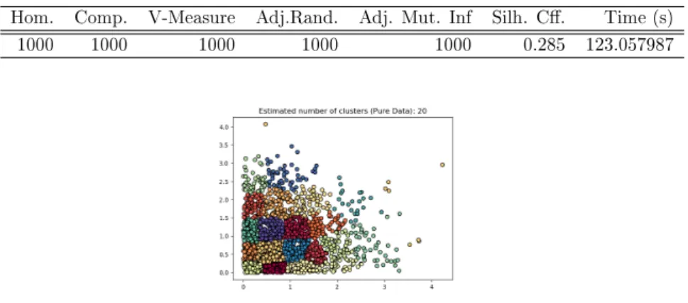
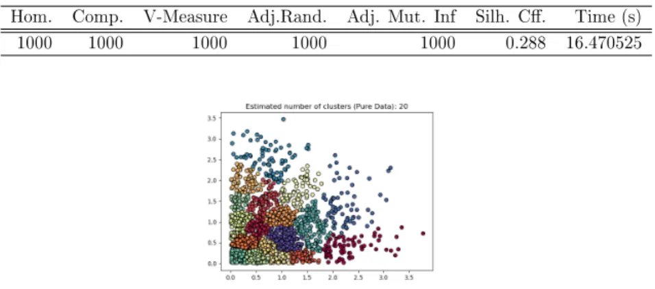
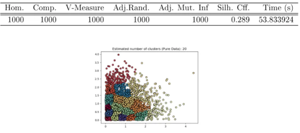
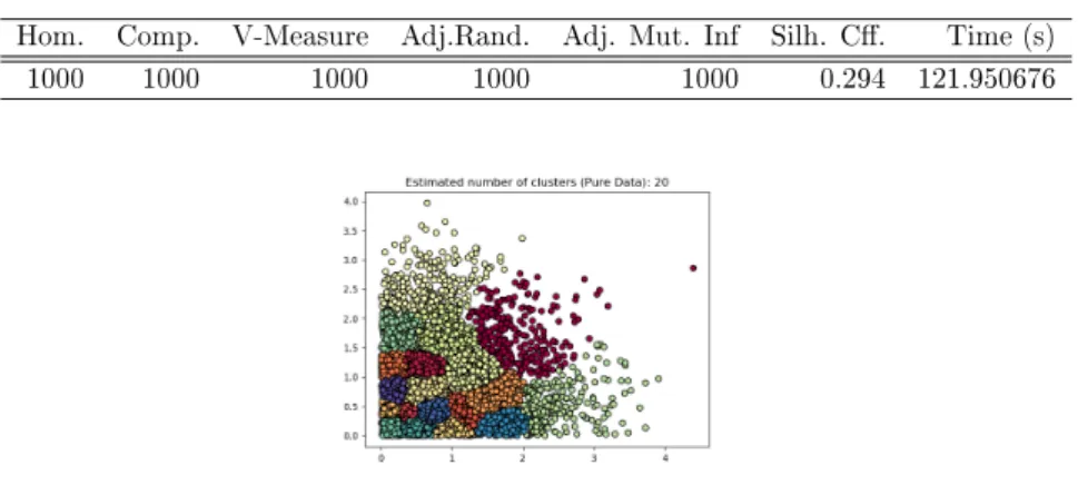
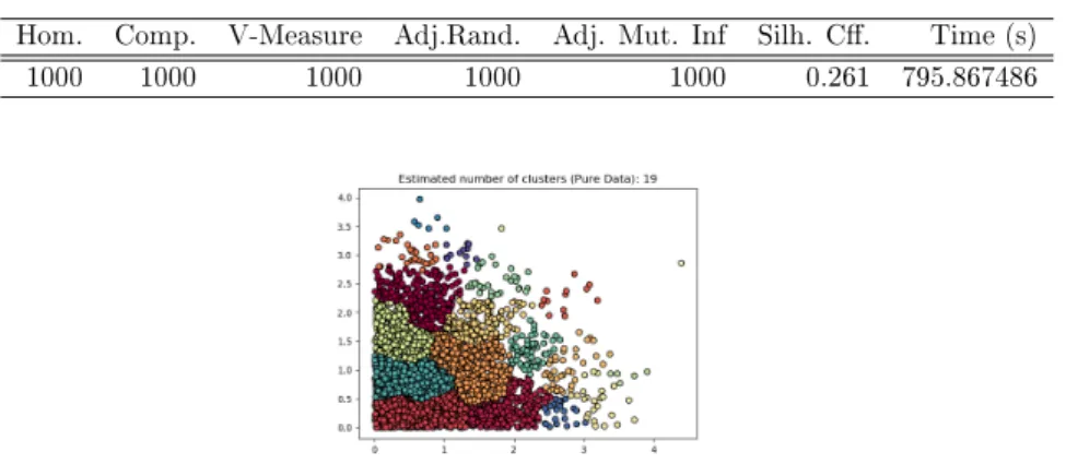
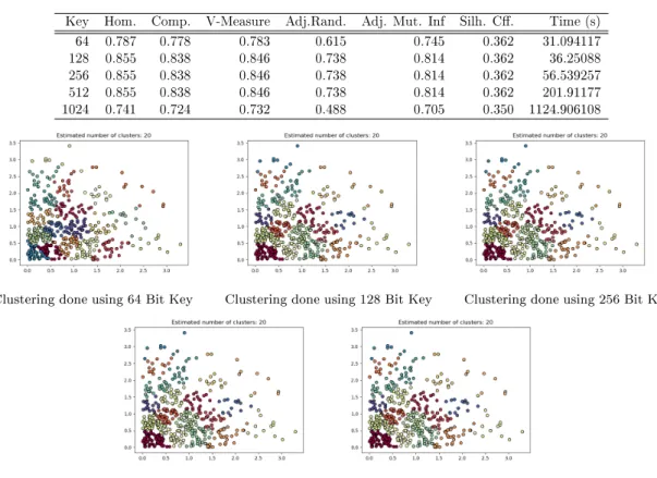
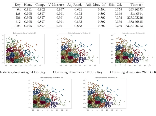
In this work, clustering methods which have been described in section 3 have been studied by running each of them on 10 dierent datasets (from 500 to 5000 rows) with using 5 dierent bit lengths of keys. Datasets are produced/chosen dierent from each other by their data and data lengths. The computer used in our experiments has limited computational capacity to calculate distance matrix especially when 512 and 1024 bit long keys are used on data which has more than 5000 rows. The data length of each dataset is also the name of the dataset (dataset 500, dataset 1000 etc.) and used key lengths vary between 64 bit and 1024 bits.
Experimental results have tables which include evaluation metric scores under the name of 00P lain/Encrypted domain clustering results00 based on the chosen dataset and
domain. Plain data results have same time result for each key length , because for plain domain encryption there is no calculation using a key. Evaluation metrics have (except silhouette coef f icient) maximum scores because of the used data is artif icial
and not real.
All algorithms have been run on python environment (as explained in section 4.1.) and all algorithm codes have been modied to create same number of clusters (20clusters)
from given data. Just in the case of Birch Algorithmon gures that show distribution
of clusters, number of clusters is as 19, because the cluster numbers are varying between 0 and 19.
Section 5. Experiments 25
5.1 Plaintext Results
5.1.1 K-Means Algorithm Results
From Table 5.1 to 5.10 and Figure 5.1 to 5.10 we will see the distribution ofplaindata
which its length varies between 500 and 5000 due to K-Means algorithm. K −M eans
algorithm forms clusters considering distancesbetween points. This algiorithm is used
generally when the data that needs to be clustered has at geometry, creating too many clusters is not necessary and created clusters are even sized.
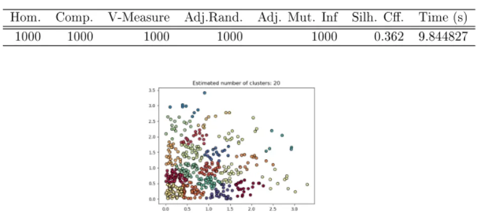
Table 5.1: Plain domain evaluation metric scores for dataset 500 Hom. Comp. V-Measure Adj.Rand. Adj. Mut. Inf Silh. C. Time (s)
1000 1000 1000 1000 1000 0.362 9.844827
Figure 5.1: Plain domain clustering for dataset 500 Table 5.2: Plain domain evaluation metric scores for dataset 1000 Hom. Comp. V-Measure Adj.Rand. Adj. Mut. Inf Silh. C. Time (s)
1000 1000 1000 1000 1000 0.350 36.957112
Section 5. Experiments 26
Table 5.3: Plain domain evaluation metric scores for dataset 1500 Hom. Comp. V-Measure Adj.Rand. Adj. Mut. Inf Silh. C. Time (s)
1000 1000 1000 1000 1000 0.359 86.728137
Figure 5.3: Plain domain clustering for dataset 1500 Table 5.4: Plain domain evaluation metric scores for dataset 2000 Hom. Comp. V-Measure Adj.Rand. Adj. Mut. Inf Silh. C. Time (s)
1000 1000 1000 1000 1000 0.352 163.580145
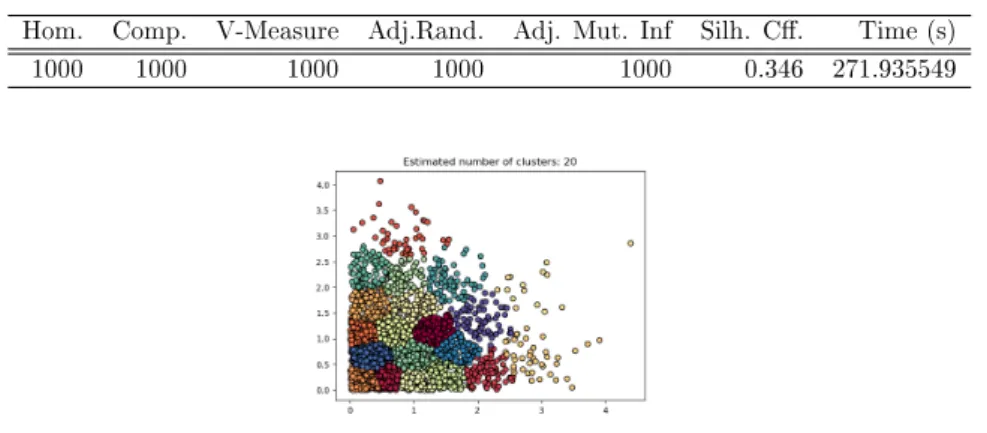
Figure 5.4: Plain domain clustering for dataset 2000 Table 5.5: Plain domain evaluation metric scores for dataset 2500 Hom. Comp. V-Measure Adj.Rand. Adj. Mut. Inf Silh. C. Time (s)
1000 1000 1000 1000 1000 0.346 271.935549
Section 5. Experiments 27
Table 5.6: Plain domain evaluation metric scores for dataset 3000 Hom. Comp. V-Measure Adj.Rand. Adj. Mut. Inf Silh. C. Time (s)
1000 1000 1000 1000 1000 0.338 413.855393
Figure 5.6: Plain domain clustering for dataset 3000 Table 5.7: Plain domain evaluation metric scores for dataset 3500 Hom. Comp. V-Measure Adj.Rand. Adj. Mut. Inf Silh. C. Time (s)
1000 1000 1000 1000 1000 0.338 623.065649
Figure 5.7: Plain domain clustering for dataset 3500 Table 5.8: Plain domain evaluation metric scores for dataset 4000 Hom. Comp. V-Measure Adj.Rand. Adj. Mut. Inf Silh. C. Time (s)
1000 1000 1000 1000 1000 0.345 1048.278932
Section 5. Experiments 28
Table 5.9: Plain domain evaluation metric scores for dataset 4500 Hom. Comp. V-Measure Adj.Rand. Adj. Mut. Inf Silh. C. Time (s)
1000 1000 1000 1000 1000 0.349 1292.195140
Figure 5.9: Plain domain clustering for dataset 4500 Table 5.10: Plain domain evaluation metric scores for dataset 5000 Hom. Comp. V-Measure Adj.Rand. Adj. Mut. Inf Silh. C. Time (s)
1000 1000 1000 1000 1000 0.340 1292.195140
Figure 5.10: Plain domain clustering for dataset 5000
5.1.2 Hierarchical Algorithm Results
From Table 5.11 to 5.20 and Figure 5.11 to 5.20 we will see the distribution ofplaindata
which its length varies between 500 and 5000 due to Hierarchical algorithm. Hierarchical
algorithm forms clusters consideringpairwise distancesbetween points. This algiorithm
is used generally when creating too many clusters is necessary and there are possible connectivity constraints to form clusters.
Table 5.11: Plain domain evaluation metric scores for dataset 500 Hom. Comp. V-Measure Adj.Rand. Adj. Mut. Inf Silh. C. Time (s)
1000 1000 1000 1000 1000 0.295 2.297151