Integrating Variable Wind Power Using a Hydropower Cascade

(1)

Peer-review under responsibility of SINTEF Energi AS doi: 10.1016/j.egypro.2015.12.339

Energy Procedia 87 ( 2016 ) 108 – 115

ScienceDirect

5th International Workshop on Hydro Scheduling in Competitive Electricity Markets

Integrating variable wind power using a hydropower cascade

Andrew Hamann

a,∗

, Gabriela Hug

a a_{Power Systems Laboratory, ETH Zurich, 8092 Zurich, Switzerland}

Abstract

In this paper, we examine the ability of a hydropower cascade to balance variability from wind power. We consider a coordinated hydro-wind system that satisfies a single power balance, and we use a real-time control scheme to optimize system operations such that wind and load curtailment is minimized. The control scheme considers system hydraulics (including dynamic tailrace elevations and water travel times) and system constraints. Generation from an individual hydropower plant is modeled using a convex piecewise planar approximation. We give results from a case study involving hydro and wind power in the Pacific Northwest region of the United States. The objective of this paper is to present a framework for evaluating how the regulation of wind generation affects hydropower operations. Our intention is to use this framework in future work to perform a systematic study of balancing capability across different hydraulic conditions, system constraints, and wind generation scenarios.

c

2015 The Authors. Published by Elsevier Ltd. Peer-review under responsibility of SINTEF Energi AS.

Keywords: hydropower, wind power, renewable generation, optimization, model predictive control, quadratic programming

1. Introduction

In recent years, there has been a sustained push to supplement and replace conventional thermal generation with wind and solar power. However, renewable generation is both intermittent and variable, and output power can only be forecasted with a certain degree of accuracy. As more wind power comes online, the variability from wind generation dominates the variability from electricity demand and stresses the power system’s ability to remain balanced [1]. Methods to address this variability include the implementation of grid-scale storage, more active demand response, and increased deployment of fast ramping and cycling natural gas generation. However, in regions with the necessary water resources, flexible hydropower plants are viewed as an ideal counterpart to variable renewable generation [2]. There are examples in the literature demonstrating the benefits of operating hydropower and wind power symbiotically to increase economic profit [3], mitigate transmission congestion [4], and reduce wind curtailment [5]. Broader, system level studies have demonstrated repeatedly that “flexibility in the scheduling of hydro generation is clearly beneficial to the integration of wind and solar resources” [1,2,6].

This paper is focused on assessing the capability of a hydropower cascade to integrate different levels of wind penetration. Specifically, we look at the sub-hourly optimization and dispatch of hydropower and wind resources in order to identify how the performance of the hydropower cascade is affected by the variability and intermittency of

∗_{Corresponding author. Tel.:}₊_{41 44 632 46 14; fax:}₊_{41 44 632 12 52.} E-mail address:[email protected]

(2)

wind power. Previous studies have indicated that the point where wind penetration begins to adversely aﬀect the total value of an integrated hydro-wind system is between 20% and 30% [1,2,7]. However, these studies have also identiﬁed the need for more detailed modeling of minute-by-minute system hydraulics and real-time constraints in order to better characterize the relationship between wind penetration and the balancing performance of the hydropower system.

The paper is organized as follows. Section 2 presents optimization and system modeling for the hydropower cascade. Section 3 introduces the Mid-Columbia hydropower system and associated dataset. Section 4 presents the results from a case study used to illustrate our methods. Section 5 concludes the paper.

2. Modeling and optimizing the hydropower cascade

Our control scheme employs model predictive control (MPC), a type of receding horizon optimal control in which a linear state space model is used to predict the reaction of a system to a set of control inputs [8]. This section discusses the optimization scheme that we developed using the MPC framework (including the hydraulic model), the approximation of power production from a hydropower plant, the objective function, and the formulation of a combined hydro-wind system power balance.

2.1. Hydraulic model

Linear, time-discrete MPC models have the general form

x(k+1)=Ax(k)+Bu(k) (1)

fork=0, . . . ,K−1 whereu(k) is the vector of control variables andx(k) is the vector of state variables. TheAand Bmatrices describe the relationship between the control inputs, current system state, and future system state. K is the discrete time-horizon over which the system is optimized. Constraints on state and control variables are explicitly incorporated into the MPC model. Additionally, since the state variable cannot change instantaneously,x(0) is a ﬁxed value reﬂecting the initial system state.

In a cascaded hydropower system, hydraulic coupling of reservoirs can be modeled with a water balance equation in which water from the upstream hydropower plant (HPP) arrives in the forebay of the downstream HPP after some travel time. Mathematically,

xj(k+1)=xj(k)− tk Ψj qj(k)+sj(k) + tk Ψj wj(k−τj)+qj−1(k−τj)+sj−1(k−τj) (2) where the natural inﬂow into the reservoir behind damjis denoted bywj(k); turbine discharge and spill through dam j

is denoted byqj(k) andsj(k), respectively; and the water level behind dam jis denoted byxj(k). There are a total ofJ

dams in the cascade.Ψjis the eﬀective surface area of the reservoir behind damj. The model is discretized bytk, the

length of the optimization interval. Thetk/Ψjterm in (2) maps water ﬂow into or out of reservoir jto a proportional

increase or decrease in the elevation of reservoir j. For hydropower cascades with multiple upstream reservoirs, the water balance equation (2) could be modiﬁed to account for inﬂows from all upstream HPPs [4].

The travel timeτjbetween dam j−1 and dam jis normalized by the optimization time steptk. Water travel times

on the Mid-Columbia are on the order of tens of minutes. In our previous work, we implicitly setτj = 0 [9]. For

modeling simplicity, we set the delay times for natural inflow, turbine discharge, and spill to be equal. Since natural inflows on the Mid-Columbia are relatively small, this assumption does not affect our modeling results. However, for other systems, the time delay for natural inflow could be different than the time delay for turbine discharge and spill. We also considered using river routing equations to model hydraulic coupling [10], but we elected not to use such a formulation because flow and elevation measurements were too noisy to fit accurate routing equations.

The state space model used in MPC relates the system state and control inputs at timekwith the system state at the next time stepk+1. Since the travel time between each dam is several times the length of the optimization time step, the formulation in (2) must be modiﬁed by introducing additional state variables that retain this information across multiple time-steps. By integrating these variables, the time delayτj 0 is modeled while only relating the state

variables at intervalskandk+1. This procedure is similar to the one used when constructing the state-space equations for a transfer function with multiple zeros [11].

(3)

The hydraulic head of a dam is the diﬀerence between the forebay and tailrace elevations, and it is one of the factors that determines how much power is generated by an HPP. (The tailrace is the water immediately downstream of a dam into which the spillway and turbines discharge.) Accurately modeling the tailrace elevation is thus very important for accurately modeling power generation, and it is well-known that the volume of water discharged into the tailrace determines its elevation [12–15]. Mathematically,

hj(k)=xj(k)−zj(k) (3)

wherehj(k) andzj(k) are the hydraulic head and tailrace elevation, respectively. We model tailrace elevationzj(k)

using an equation of the form

zj(k+1)=αj·

qj(k)+sj(k)

+γj·xj+1(k)+z0j (4)

whereαj,γj, andz0j are parameters ﬁtted using ordinary least-squares regression. Tailrace elevation is a function of

both the flow into the tailrace (qj(k)+sj(k)) and the elevation of the downstream reservoirxj+1. In the case of the final HPP in the cascade, there is no downstream reservoir. Hence, the equation definingzJwill not have aγJorxJ+1term. Since the proposed model contains the affine termz0

j, we compute the linear term using the state space model and add

the aﬃne term when we compute the tailrace elevation in meters above sea level [9].

Limits on the state and control variables are also incorporated into the optimization problem, i.e.,

qmin_j ≤qj(k) ≤qmaxj (5)

smin

j ≤sj(k) ≤smaxj (6)

wpred_j (k)≤wj(k)≤wpred_j (k) (7)

xmin_j ≤xj(k) ≤xmaxj (8)

where (5) and (6) limit turbine discharge and spill to fixed minimum and maximum values, and (7) limits natural inflow to values determined by a forecast. Limits on forebay elevation (8) are dictated by the regulatory, environmental, and operational constraints specific to each HPP or section of the river.

2.2. Modeling the hydropower production function

The amount of gross electrical power extracted from a hydro turbine-generator is a non-linear function of turbine eﬃciencyηt, generator eﬃciencyηg, turbine dischargeq, and hydraulic headh[16]. This is known as the hydropower

production function (HPF). Mathematically,

p(ηt, ηg,q,h)=κ·ηt·ηg·q·h (9)

wherepis the gross electrical power produced by the generator andκis a conversion constant. It may also contain additional terms, such as losses associated with the friction of water in the penstocks or trash racks [13,16]. The primary contribution of our previous work lies in how we linearize the HPF and integrate it into an MPC optimiza-tion framework, maintaining the speed advantage of quadratic programming while making no assumpoptimiza-tions about the closed-form structure of the HPF [9]. We use the same modeling approach in this paper.

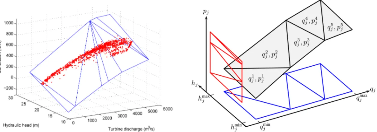
The linearization process is a standard segmented regression with continuity and convexity constraints in which the number and position of each section is pre-selected [17]. In the regression, the covariates are the turbine discharge q, hydraulic headh, and an intercept term. Each partition is deﬁned as the triangle formed by a triplet of (q,h) coordinates. The regression problem is a constrained least-squares quadratic program with dimension proportional to the number of partitions. A constraint in the regression ensures that the function is concave in the ˆqdirection for all values ofh. The left side of Fig. 1 shows the approximated HPF for Wells Dam.

We introduce auxiliary variables into the optimization problem to account for the piecewise planar form of our approximation. In short, each section of the approximated HPF is assigned its own discharge and power variable. These discharge and power variables are then summed, less their lower limits, to obtain the total discharge and power generation for each HPP. The right side of Fig. 1 illustrates how these variables are assigned to each section of the piecewise planar HPF approximation. The mathematical relationships describing how the approximated HPF is incorporated as linear constraints into the full optimization problem are detailed in our previous work [9].

(4)

q1 j, p1j q2 j, p2j q3 j, p3j q4 j, p4j q5 j, p5j qmin j qmax j hmin j hmax j qj hj pj

Fig. 1. (a) Approximated hydropower production function for Wells Dam; (b) Illustrative diagram of a piecewise linear HPF with ﬁve sections.

2.3. Power balance equation

In our simulations, the hydropower cascade is assumed to be controlled by a central coordinating entity. In the absence of wind power, the cascade is operated to meet the aggregate generation request of the HPP stakeholders. Mathematically,

J

j=1

pj(k)=phydroload(k) (10)

where phydroload(k) is the electricity demand satisﬁed by the cascade during intervalk. Data of historical system operations is used to compute the system demandphydroloadfor use in our simulations.

In the combined hydro-wind system, wind generation is added to the power balance. An equivalent amount of load energy is also added to the power balance, satisfying the property

N n=1 pwind(n)= N n=1 pwindload(n) (11)

wherepwind(n) is the wind generation in periodn,pwindload(n) is the additional load used to offset wind generation in periodn, andNis the length of the simulation period (e.g., for a one-day simulation with five-minute resolution, N = 288). This constraint ensures that each additional unit of wind energy is offset by an additional unit of load ensuring, structuring the problem such that the hydropower cascade generates approximately the same amount of energy for the hydropower stakeholders (i.e.,phydroload) while operating in a more flexible fashion. The relationship (11) will not necessarily hold in the simulation if load or wind is curtailed.

Constraint (10) is then updated to be

J

j=1

pj(k)+(k)=phydroload(k)+pwindload(k)−pwind(k) fork=0,1, ...,K−1 (12) where(k) is the amount of curtailed wind generation (if negative) or the amount of curtailed load (if positive). If the hydropower cascade must over-generate relative to the net load,(k) will be negative and wind will be curtailed. If the hydropower cascade must under-generate relative to the net load,(k) will be positive and load will be curtailed. 2.4. Objective function

Our objective function is to minimize turbine discharge and spill. The objective function can be written as min qj,sj, ⎧⎪⎪ ⎪⎨ ⎪⎪⎪⎩ K−1 k=0 J j=1 aj·qj(k)2+cj·sj(k)2 + K−1 k=0 d·(k)2⎫⎪⎪⎪⎬_⎪⎪⎪⎭ (13)

(5)

whereaj,cj, anddare scalar weights. Qualitatively, the goal of the proposed scheme is to minimize the amount

of water needed to satisfy the system power balance. We chose to use a quadratic objective function because it reduces the ramping of turbine discharge and spill without explicitly weighting those variables. In addition, it creates a strongly convex optimization problem with a single optimal solution whereas a linear program could have multiple globally optimal solutions. We choose our weights such that

aj=cj= ηj ηj+1 · Ψj+1 Ψj 2 daj (14)

forj=1, . . . ,J, whereηjandΨjare, respectively, the powerhouse eﬃciency and forebay surface areas for HPPj. This

objective function is designed to favor the transfer of water from low efficiency, large forebay HPPs to high efficiency, small forebay HPPs. This maximizes system hydraulic head and increases total system conversion efficiency. In the case of the final dam in the cascade, there is no downstream forebay or HPP. Hence, we choose the weightsaJ (with

cJ =aJ) large respective to the other weights on turbine discharge. Additionally, we heavily penalizeby making

dvery large, discouraging the curtailment of load and wind unless it is absolutely necessary to maintain the power balance constraint (12). Actual weights used in our case study are given in Section 4.

3. Mid-Columbia hydropower system and associated wind generation

The hydropower cascade of interest is the Mid-Columbia hydropower system, located on the Columbia River in eastern Washington. It consists of seven hydropower plants, and has a nameplate capacity of approximately 14 GW. Due to the intricacies of the coordination policy currently in place, this research focuses on the five municipal dams in the system. These five dams have a nameplate capacity of approximately 4 500 MW. They are operated by three county-level public utilities. Stakeholders in each HPP include many different private and public power utilities and energy companies.

Working with local utilities, we were provided with system data for 2012 and parts of 2013. This data includes timestamped measurements of turbine discharge, spill, forebay and tailrace elevation, and power generation for each hydropower plant. The data also includes real-time minimum and maximum limits for forebay elevation, turbine discharge, and generator ramping. This data has enabled us to develop an accurate, valid, and useful model of the Mid-Columbia system. Data was available to us in one- and five-minute resolution. (The case study discussed in the following section uses the five-minute data.) In addition to the data supplied to us, we determined fish spill constraints using publicly available environmental records and FERC filings. Natural inflows were taken from gauge data made publicly available by the United States Geological Survey with 15-minute resolution1_{. Natural inflows and sideflows} on the Mid-Columbia River are usually a small percentage of the flow on the main stem river, and these flows do not vary substantially on a minute-by-minute basis.

For wind, the Bonneville Power Administration (BPA) makes wind generation data available on their website, and this data is supplied in five-minute intervals dating back many years2_{. BPA manages the federally owned dams in} the Columbia River Basin. In addition, it operates a large transmission network to transmit that power from sparsely populated areas to load centers on the West Coast. The BPA balancing area has a large and increasing amount of interconnected wind generation, and the problem of how to balance this wind is a pressing issue for BPA and other utilities in the region. The colocation of the Mid-Columbia system and a large amount of wind generation makes it an ideal for studying beneficial hydro-wind coordination [2,7]. Additionally, conducting our simulations using real wind data enables us to match seasonal variations in wind generation with different hydraulic conditions.

Power forecasts, for both load and wind generation, were taken to be accurate but not perfect. Forecasts were developed by taking the actual predicted wind generation or system load at the top of each hour and using those values to generate the forecast for the time horizon of interest. For example, suppose it is 8:30, the optimization time horizon is two hours, and the optimization time steptkis ﬁve minutes. Using the wind generation (or electricity

demand) at 8:30, 9:00, 10:00, and 11:00, a piecewise linear forecast can be formulated. Then, the forecast for the two

1_http:_//_{waterdata.usgs.gov}_/_usa_/_nwis_/_rt

(6)

hour time horizon is computed by interpolating that piecewise linear forecast every ﬁve minutes from 8:30 to 10:25. Future work may utilize improved forecasting techniques for load and wind power.

4. Case study results

We chose a period of five days (120 hours) in July 2012 for which we had five-minute Mid-Columbia operations data. We used unscaled BPA wind generation data from the same time period, and scaled BPA balancing area load for the additional wind load. This time period is interesting because flows on the Columbia River were substantially higher than normal. This resulted in more hydraulic generating capacity (and more spill) than in lower flow years. Additionally, all five dams had minimum spill limits for fish passage reasons. In the optimization problem, the optimization intervaltk was five minutes and time horizonK was three hours (K = 36). Simulations were run in

MATLAB. The optimization problem was solved using the qp-minos solver, accessed via the TOMLAB interface. Each optimization problem took a few seconds to solve.

We ran two simulations: one with wind and one without. In both cases, the objective function and all constraints were the same; the only difference was the addition of wind power and additional electricity demand in the hydro-wind scenario. Basic results are shown in Table 1, including average flows and average spill for the historical, hydro-only, and hydro-wind scenarios. Figure 2 shows the turbine discharge and spill for the time period of interest. Since this was a high flow period and wind curtailment was heavily penalized, turbine discharge was ramped to follow load whereas spill was ramped to keep each forebay below its maximum elevation limit. Figure 3 illustrates how load was curtailed when there was no remaining generation capacity on the system and each HPP was operating at its maximum turbine discharge. (In lighter load periods, it is conceivable that wind would be curtailed if all HPPs were operating at their minimum turbine discharge limits and wind was over-generating. This situation did not occur in this particular simulation, however.) Figure 3 also demonstrates the intermittency of wind, with generation ramping down from 3000 MW to nothing in the course of a few hours.

There are two primary criteria by which to evaluate the performance of a hydro-wind system. The ﬁrst is: how much more (or less) do HPPs need to ramp their generation when balancing wind power? While small ramps are generally not problematic, large ramps that require HPPs to cycle individual units are a key source of excessive wear and tear on turbine-generators. Some HPPs could also bear a disproportionate burden of wind integration costs if ramping is not equally distributed across the system. As shown in Table 2, ramping for each HPP was higher in the hydro-wind scenario compared to the hydro-only scenario, and ramping was not allocated evenly. The ramping score does not directly estimate unit cycling, but increased ramping will likely cause additional cycling of individual turbine-generator units.

The second question is: when balancing is infeasible, how much load or wind is curtailed? In this simulation, the total load on the hydro-wind system for the ﬁve-day simulation period was 4884 MWavg. This load was satisﬁed by 2874 MWavg of hydropower generation, 1664 MWavg of wind generation, and 346 MWavgof load curtailment. There was no wind curtailment. Peak wind generation was 3838 MW, and peak load was 5396 MW. Wind energy penetration was approximately 34%, and wind capacity penetration was 71%. Approximately 7% of load energy was curtailed, and load curtailment occurred primarily due to capacity constraints on hydropower generation. Peak load curtailment was 1563 MW, and it occurred at the same time as peak load. At that time, approximately 30% of load was

Table 1. Simulation inputs and results, with elevationsxin meters, surface areasΨin km2_{, and ﬂows in m}3_/_{s. Flows have been rounded.}

System Parameters and Limits Mean Turbine Discharge Mean Spill j Name xmin xmax Ψ η a Hist. Hydro H+W Hist. Hydro H+W 1 Wells 235.0 238.0 41 0.85 0.67 4850 3740 3940 2410 3510 3320 2 Rocky Reach 214.3 215.5 36 0.90 0.13 4590 4520 3750 2730 2780 3550 3 Rock Island 185.6 186.8 12 0.84 23 5700 3710 3840 1770 3740 3610 4 Wanapum 171.9 174.2 57 0.84 0.25 3480 3920 3190 4350 3860 4590 5 Priest Rapids 146.8 148.1 28 0.83 100 2730 3920 3780 5160 3900 4030

(7)

Fig. 2. (a) Turbine discharge shown for the historical, hydro-only, and hydro-wind scenarios; (b) Spill for the same scenarios. Due to high ﬂows and the penalty on wind curtailment, turbine discharge was ramped to follow net load and spill was ramped to satisfy hydraulic constraints.

Fig. 3. (a) Hydro load and wind load, combined, comprise the system power balance for the combined hydro-wind system; (b) The breakdown of how the power balance was satisﬁed (wind generation, hydro generation, and load curtailment). There was no wind curtailment, but there were periods where load was curtailed because there was little wind generation and each HPP was operating at its maximum turbine discharge limit.

being curtailed. Load curtailment results in additional spilled energy for the cascade, since water that was used for generation in the hydro-only case is no longer needed because load curtailment has “generated” that power instead (by reducing the electricity demanded of the hydro-wind system). The amount of spilled energy is reflected in the energy deficit for Wanapum and Rocky Reach HPPs, as they produced approximately one-fifth less energy in the hydro-wind scenario compared to the hydro-only scenario. These statistics are shown in Table 2.

Table 2. Simulation results, with power given in MW. The turbine discharge ramping score does not have units, but a lower score indicates

less ramping. Mean turbine discharge and spill are converted to power using a conversion factor. The deﬁcit column is the diﬀerence in energy

generation between the hydro-only and hydro-wind scenarios, given in MWavg. A negative number indicates that more energy was generated in the

hydro-only scenario.

Ramping Score Mean Turbine Power Mean Spill Power

j Name Hist. Hydro H+W Hist. Hydro H+W Hist. Hydro H+W Deﬁcit 1 Wells 9.3 7.8 24.3 657 507 533 327 476 450 26 2 Rocky Reach 9.4 17.0 26.6 1216 1199 994 724 737 942 -204 3 Rock Island 6.6 5.6 31.3 480 313 324 149 315 304 11 4 Wanapum 10.9 2.9 15.5 789 889 723 985 876 1040 -166 5 Priest Rapids 21.6 6.0 13.9 466 669 645 881 665 688 -24

(8)

5. Conclusion

This paper presented a method for simulating the real-time operations of a combined hydro-wind system. A short case study was presented using the Mid-Columbia hydropower system as a test system. The results from the case study showed that HPP ramping increased due to increased volatility in net load. Additionally, during low wind periods, load was curtailed as a result of insufficient hydropower generation capacity. In the future, our intention is to use the presented framework to perform a large-scale, systematic study of balancing capability across different hydraulic conditions, system constraints, and wind generation scenarios. We will analyze how operating a hydro-wind system affects system ramping, system value, load and wind curtailments, and the allocation of turbine discharge and ramping across the HPPs in the cascade. Specific attention will be paid to how and on what timescales wind generation is firmed. Additionally, we intend to investigate objective functions that operate the cascade in such a way that flexibility is prioritized over capacity.

Acknowledgements

Much of this research was performed at Carnegie Mellon University while both authors were affiliated with the Department of Engineering and Public Policy. The authors would like to thank the University and the Department for their support. In addition, this research was funded in part by the Office of Energy Efficiency and Renewable Energy (EERE), U.S. Department of Energy, under Award Number DE-EE0002668 and the Hydro Research Foundation; the Robert W. Dunlap Graduate Fellowship, awarded by the Steinbrenner Institute for Environmental Education and Research; and the Electric Power Research Institute under Project 1-105910-01-01.

References

[1] The Western Wind and Solar Integration Study Phase 1. Tech. Rep. NREL/SR-550-47434; National Renewable Energy Laboratory; Golden,

Colorado; 2010.

[2] Acker T. IEA Wind Task 24: Integration of Wind and Hydropower Systems. Tech. Rep. NREL/TP-5000-50181; National Renewable Energy

Laboratory; 2011.

[3] Castronuovo ED, Lopes JAP. On the optimization of the daily operation of a wind-hydro power plant. Power Systems, IEEE Transactions on 2004;19(3):1599–606.

[4] Matevosyan J, Olsson M, S¨oder L. Hydropower planning coordinated with wind power in areas with congestion problems for trading on the spot and the regulating market. Electric Power Systems Research 2009;79(1):39–48.

[5] Hug-Glanzmann G. A hybrid approach to balance the variability and intermittency of renewable generation. In: PowerTech, 2011 IEEE Trondheim. Trondheim, Norway; 2011, p. 1–8.

[6] Koritarov V. Modeling and analysis of value of advanced pumped storage hydropower in the United States. ANL/DIS-14/7; Argonne National

Laboratory; 2014.

[7] Clement MA. A methodology to assess the value of integrated hydropower and wind generation. Master’s thesis; University of Colorado Boulder; 2012.

[8] Glanzmann G, von Siebenthal M, Geyer T, Papafotiou G, Morari M. Supervisory water level control for cascaded river power plants. In: Workshop on Hydro Scheduling. Stavanger, Norway; 2005,.

[9] Hamann A, Hug G. Real-time optimization of a hydropower cascade using a linear modeling approach. In: Power Systems Computation Conference (PSCC). Wrocław, Poland; 2014,.

[10] Souza TM, Diniz AL. An accurate representation of water delay times for cascaded reservoirs in hydro scheduling problems. In: Power and Energy Society General Meeting, 2012 IEEE. 2012, p. 1–7.

[11] Chen CT. Linear System Theory and Design. Third ed.; New York: Oxford University Press; 1999.

[12] Alley WT. Hydroelectric plant capability curves. Power Apparatus and Systems, IEEE Transactions on 1977;96(3):999–1003.

[13] Arce A, Ohishi T, Soares S. Optimal dispatch of generating units of the Itaipu hydroelectric plant. Power Systems, IEEE Transactions on 2002;17(1):154–8.

[14] Diniz AL, Maceira MEP. A four-dimensional model of hydro generation for the short-term hydrothermal dispatch problem considering head

and spillage eﬀects. Power Systems, IEEE Transactions on 2008;23(3):1298–308.

[15] Lima RM, Marcovecchio MG, Novais AQ, Grossmann IE. On the computational studies of deterministic global optimization of head dependent short-term hydro scheduling. Power Systems, IEEE Transactions on 2013;28(4):4336–47.

[16] Cordova MM, Finardi EC, Ribas FAC, de Matos VL, Scuzziato MR. Performance evaluation and energy production optimization in the real-time operation of hydropower plants. Electric Power Systems Research 2014;116:201–7.